WORKING PAPER SERIES
Universidade dos Açores Universidade da Madeira
CEEAplA WP No. 04/2004
Demand Shocks and Productivity Growth
António Gomes de Menezes
Demand Shocks and Productivity Growth
António Gomes de Menezes
Universidade dos Açores (DEG)
e CEEAplA
Working Paper n.º 04/2004
Novembro de 2004
CEEAplA Working Paper n.º 04/2004
Novembro de 2004
RESUMO/ABSTRACT
Demand Shocks and Productivity Growth
This paper presents evidence on the relationship between cyclical shocks and
productivity growth, for 20 2-digit SIC US manufacturing industries and a set of
monetary policy, .scal policy, and oil price shocks. The paper uses as a easure
of productivity change a Solow residual corrected for a wide range of
non-technological e¤ects due to imperfect-competition, non-constant returns to
scale, and cyclical utilization rates of capital and labor services. The empirical
framework identi.es policy shocks independently of productivity measurement
issues via a two-step procedure. While the typical industry shows weak
responses of productivity to the shocks considered, in some industries
temporary contractionary policy shocks lead to increases in productivity. In
addition, the results reveal that there are localized asymmetries, with
contractionary policy shocks having larger produtivity e¤ects than their
expansionary counterparts. The results support the thesis that job reallocation is
an important channel linking contractionary policy shocks and productivity
growth. These results support the pit-stop view of downturns.
António Gomes de Menezes
Departamento de Economia e Gestão
Universidade dos Açores
Rua da Mãe de Deus, 58
9501-801 Ponta Delgada
Demand Shocks and Productivity Growth
António Gomes de Menezes University of the Azores and CEEAplA
November 2004
Abstract
This paper presents evidence on the relationship between cyclical shocks and productivity growth, for 20 2-digit SIC US manufacturing industries and a set of monetary policy, …scal policy, and oil price shocks. The paper uses as a measure of productivity change a Solow residual corrected for a wide range of non-technological e¤ects due to imperfect-competition, non-constant returns to scale, and cyclical utilization rates of capital and labor services. The empirical framework identi…es policy shocks independently of productivity measurement issues via a two-step procedure. While the typical industry shows weak responses of productivity to the shocks considered, in some industries temporary contractionary policy shocks lead to increases in productivity. In addition, the results reveal that there are localized asymmetries, with contractionary policy shocks having larger produtivity e¤ects than their expansionary counterparts. The results support the thesis that job reallocation is an important channel linking contractionary policy shocks and productivity growth. These results support the pit-stop view of downturns.
University of the Azores, Department of Economics and Management, 9501-801 Ponta Delgada, Portugal. E-mail: [email protected]. I thank participants at seminars at Boston College, University of Alberta and Simon Fraser University for helpful comments.
1
Introduction
Macroeconomic theory has traditionally neglected the e¤ects of cycles on productivity growth. Re-cently, however, several papers in the endogenous growth literature have challenged this stance and have proposed theories on the e¤ects of cycles on productivity growth. To date, the empirical evidence is mixed and on balance inconclusive (Aghion and Howitt (1998, Ch. 8)). A characteriza-tion of the literature on cycles and productivity growth as ‘some stories, no facts’, while somewhat harsh, is on the mark. These developments, combined with recent advances in the measurement of productivity, provide the impetus for renewed interest in empirical work on the relationship between cycles and productivity growth. This paper studies the productivity e¤ects of a set of cyclical shocks for 20 2-digit SIC US manufacturing industries, from 1972:2 to 1992:4. The paper focuses on the arguments recently formalized by Aghion and Saint-Paul (1998).
Aghion and Saint-Paul (1998) argue that some productivity improving activities are disruptive, in the sense that …rms must sacri…ce some output and pro…ts to implement them. Hence, during temporary demand downturns the opportunity cost of investing in such disruptive productivity improving activities is lower and …rms invest more in these activities, which results in productivity growth. As a corollary of this reasoning, we follow the literature and use the label "Opportunity Cost View" of recessions henceforth. Examples of such activities may include job reallocation, managerial reorganizations, experimentation with new technologies, and training.
Some authors, namely Gali and Hammour (1992) and Saint-Paul (1993), have found empirical evidence that supports such view of recessions. Gali and Hammour and Saint-Paul study the pro-ductivity e¤ects of demand shocks by means of bivariate VARs, with propro-ductivity change measured by the Solow residual and a cycle indicator, typically an employment rate. They identify demand shocks as those shocks with no within-period e¤ect on productivity. Gali and Hammour use quar-terly and annual data for the US manufacturing sector, while Saint-Paul uses aggregate annual data for a sample of OECD countries. Both studies …nd that a negative demand shock leads to an increase in productivity. However, these pieces of evidence su¤er from important shortcomings that stem from measurement of productivity, identi…cation of the demand shocks, and interpretation issues of the competing stories relating cycles and productivity growth.
On the measurement issues, studies like Basu et al. (1999) demonstrated that the Solow residual is contaminated by non-technological e¤ects, which render it a polluted measure of productivity growth. In addition, these non-technological e¤ects are highly correlated, both contemporaneously and dynamically, with shocks to activity, and hence must be controlled for in studies of the re-lationship between cyclical demand shocks and productivity growth. On the identi…cation issues,
the identifying restriction that it takes at least one period for the productivity improving activities to have a noticeable impact on productivity is certainly ad-hoc and less defensible for annual data than for quarterly data. More to the point, even if demand shocks have no within-period e¤ect on true productivity, they may have on the Solow residual.
This paper tackles these issues heads on. First, it uses as measures of productivity change Solow residuals corrected for all non-technological e¤ects believed to be of empirical importance and investigates the robustness of the results for many alternative speci…cations of productivity change. Second, the identi…cation of demand shocks is achieved independently of the measurement of productivity. In addition, the demand shocks identi…ed have concrete structural interpretations: they are monetary policy and …scal policy shocks. To achieve identi…cation of monetary policy shocks, the paper borrows from Christiano, Eichenbaum and Evans (2000) and Romer and Romer (1997), and of …scal policy shocks from Rotemberg and Woodford (1992) and Perotti and Blanchard (2002).
There are at least three reasons to focus on these shocks. First, for the Opportunity Cost View to be e¤ective, the downturn in the demand that …rms face has to be transitory since if permanent then both the costs and bene…ts of the productivity improving activities change in an equal manner, leaving the optimal investment decision in these activities unchanged. Moreover, what matters is whether …rms perceive the downturn to be transitory or permanent. If …rms correctly identify the cause of the downturn as temporary and common to the entire economy, they may want to engage in productivity improving activities to take advantage of the temporary slack before the economy picks up again. This motivates us to use economy-wide shocks, such as policy shocks, and avoid sectoral speci…c shocks, such as to relative prices, since it is more reasonable to argue that …rms expect the former to be temporary while the latter may be speci…c and permanent. Second, by studying di¤erent demand shocks we can analyze the responses of the real interest rate and of job reallocation to the di¤erent shocks, which according to the Opportunity Cost View, as argued below, have a role in the relationship between cyclical demand shocks and productivity change. Third, it may be of independent interest to analyze the productivity e¤ects of monetary policy and …scal policy shocks at the sectoral level. In this sense, this paper also provides further insight into whether monetary and …scal policy shocks have lasting real, productivity e¤ects.
On the interpretation issues, whereas the Opportunity Cost View predicts that temporary contractionary shocks may have positive productivity e¤ects, learning-by-doing (Stadler (1990)) and capital market imperfections (Stiglitz (1993)) theories predict the opposite, which complicates matters, since, ideally, empirical tests of the Opportunity Cost View ought to reveal its absolute empirical relevance in addition to its relative empirical relevance vis à vis the competing theories.
This point motivates the design of thorough and direct tests of the Opportunity Cost View. The paper attempts to do this by looking at the roles of the real interest rate and of job reallocation, and the distinct productivity e¤ects of shocks to demand and to supply conditions. In a companion paper (Menezes (2004)), we extend the Aghion and Saint-Paul (1998) model and show that: (1) supply shocks have no e¤ects on productivity growth; and (2) transitory demand downturns have positive e¤ects only if the real interest rate is not too countercyclical. The …rst result owes to the fact that supply shocks matter essentially to intra-temporal decisions, and not to inter-temporal decisions, such as the decision to invest in productivity improving activities. The second result holds because if the real interest rate increases enough during transitory demand downturns, then all investment activities decrease, regardless of their temporarily low opportunity cost. These extensions are meaningful since they guide our empirical strategy, as discussed below.
The result that supply shocks have no e¤ects on productivity growth implies that we must separate demand shocks from supply shocks, which, incidentally, we are not guaranteed to obtain from simple VAR identi…cation strategies, as pursued in Gali and Hammour and in Saint-Paul. Also note that this result is in contrast to the competing theories which are silent with respect to the demand vs. supply nature of the shocks. For this purpose, the paper uses as a measure of supply shocks oil price shocks, following Hamilton (1985) and Davis and Haltiwanger (1999).
The second result, that the cyclicality of the real interest rate has a …rst-order e¤ect on the main implications of the Opportunity Cost View, motivates us to look at the joint behavior of di¤erent demand shocks and of the real interest rate, because the Opportunity Cost View unambiguously predicts that productivity growth is stronger after transitory demand downturns associated with decreases in the real interest rate than after transitory demand downturns associated with increases in the real interest rate. We pursue this line of investigation by considering di¤erent demand shocks. Another novelty in the paper is the consideration that contractionary and expansionary de-mand shocks may have di¤erent productivity e¤ects. In Aghion and Saint-Paul (1991), only con-tractionary demand shocks have positive productivity e¤ects, while expansionary demand shocks have no e¤ects on productivity at all. Note that this asymmetry is not predicted by the competing theories, and, hence, looking at asymmetries constitutes a more thorough test of the Opportunity Cost View and helps us with the interpretation issues. Finally, the paper investigates the empirical role of job reallocation as a link between demand shocks and productivity growth.
The paper is organized as follows. Section 2 lays out the framework used to measure productivity change. Section 3 spells out the identi…cation of the shocks and the estimation of the Impulse Response Functions (IRFs) of productivity to these shocks. Section 4 documents and interprets the main results. Section 5 o¤ers some …nal remarks. The Appendix describes the data.
2
Empirical Framework
2.1 Basic Strategy to Measure Productivity Growth
Under the Solow assumptions of competitive markets, constant returns to scale, proper measure-ment of the inputs, and homogeneous production function, TFP growth and the Solow residual coincide, with the Solow residual interpreted as a shift in the underlying production function. However, and following the work by Hall (1990), a burgeoning literature vigorously demonstrated that the Solow residual should not be interpreted as a pure measure of productivity change (Basu et al. (1999)), unless proper account is taken of the non-technological e¤ects introduced into the Solow residual by the violation of the Solow assumptions. More to the point, these non-technological e¤ects are highly correlated with shocks to activity and hence cannot be treated as classical mea-surement error in the context of this paper.
While there is no agreement in the literature on how to take account of these non-technological e¤ects, there is wide agreement on the need to do so since the properties of the Solow residual change in a dramatic fashion after one controls for varying rates of input utilization, non-constant returns to scale, and imperfect competition in product markets. This literature has uncovered the following stylized facts: the corrected Solow residual, when compared to its uncorrected counterpart, displays lower implied probability of technological regress; lower volatility relative to output growth; and lower contemporaneous correlation with input and output growth. In addition, the typical US manufacturing industry exhibits constant or near constant returns to scale and a substantial amount of factor hoarding during the cycle. These characteristics can be thought of as constraints that must be satis…ed by candidate measures of productivity change (King and Rebelo (1998), Burnside, Rebelo, and Eichenbaum (1995) and Shapiro (1996))).
It seems desirable then to employ a correction framework that readily accommodates a wide spectrum of non-technological e¤ects in the original Solow residual, regardless of their sources, while leading to a corrected Solow residual in conformity with the …ndings of other independent studies.
Having the ability to study the e¤ects of the shocks of interest on productivity for each plausible correction scheme allows one to ask: for which range of this spectrum of plausible corrections does a particular result obtain? If the result obtains for the entire spectrum (all plausible corrections) then one should regard this result as independent of the correction procedure. If the answer to a particular question varies over this spectrum, then one has to integrate the di¤erent answers over all parts of the spectrum, weighting them according to their empirical plausibility, albeit in an informal manner.
2.2 A Framework to Measure Productivity Growth
Each 2-digit SIC manufacturing sector is described by a production function of the form:
Yit= AitFi( itHitNit; UitKit) (1)
where Yit is real value added, Ait is an index of the state of technology and measures TFP, Nit
is labor employees, Hit is hours worked per labor employee, Kit is the capital stock, and Fi is a
homogeneous function of some degree i. Let Lit HitNit be total labor hours worked. Firms may
change the contribution of the inputs in the short run by varying the utilization rates of labor and capital services, it and Uit, respectively.
Hall (1990) assumes that the …rm solves a cost minimization problem and derives TFP growth rate:
dait= dyit i[ it(dlit+ d it) + (1 ( it= i) it)(dkit+ duit)] (2)
where x ln X, it is the markup ratio, and it is the share of total revenue that accrues to labor
services. Equation (2) involves the unobserved series d it, duit, it, and parameter i. To render
(2) operational we employ proxies for the series d itand duit and allow the parameter i and series
it to vary within a reasonable range (discussed below).
The studies that have used proxies for duitconsidered data on electricity consumption (Burnside
et al. (1995)), shift work (Shapiro (1996)), workweek of capital (Shapiro (1996)), and functions of labor variables (Evans (1992)). We follow Burnside et al. (1995) and assume dkit+ duit deit,
where deit is the growth rate of industrial electricity consumption. Note that deit should capture
all intensive margins of adjustment that …rms may have at their reach when trying to vary the contribution of capital services; that hoarding of electricity does not pose a problem; that the sectors covered on the empirical exercises presented in this paper are all manufacturing sectors, where this assumption is a priori fairly innocuous; and that data on industrial electricity consumption are available at the quarterly frequency.
For d it we follow Gordon (1990). De…ne Lit itLit as e¤ective labor services. Assume that
itis a variable stationary around one (say, ‘e¤ort’). Let littrendand ltrendit be stationary deviations
from a common trend. Gordon assumes that a fraction 'i of the changes in littrend takes the form of changes in the labor utilization rate: it = 'ilittrend. Hence, it = ('i=(1 'i)) littrend, and, …nally, dlit= dlit+ ('i=(1 'i))dlittrend. In practice we use micro evidence on 'i found in the work
of Fay and Medo¤ (1985) who report an average value of 'iequal to 0.21 for the US manufacturing sector. However, we allow 'i to take on values f0; 0:1; 0:2; 0:3g, with the role of e¤ort increasing in 'i. The trend term is obtained by applying the Hodrick-Prescott …lter to measured hours, with
= 1600.
We let ( it= i) vary between 1 and 1= it, where the lower bound follows from the second-order
condition for pro…t maximization and the upper bound from the imposition of nonnegative returns on e¤ective capital services.1
As we try di¤erent TFP speci…cations, we get di¤erent IRFs to each shock considered. Section (4) discusses the sensitivity of the IRFs to the alternative speci…cations of TFP. Here we focus on the di¤erences in widely studied properties of the Solow residual brought about by changing the TFP speci…cation, as illustrated by Table 1 (where (x; y) is the correlation coe¢ cient between x and y, and x is the standard deviation of x). For brevity, we focus on the typical industry,
reasonably represented by the aggregate manufacturing sector. Many other speci…cations were also considered, but the speci…cations presented in Table 1 seem to encompass all the relevant ones.
Table 1 ('i; i= i) = 0; 1 0; 1:2 0:1; 1 0:1; 1:2 0:2; 1 0:2; 1:2 0:3; 1 0:3; 1:2 Prob(dait< 0) 9:6% 9:6% 16:8% 13:2% 19:2% 19:2% 24:1% 25:3% (dait; dyit) 0:20 0:15 0:00 0:09 0:23 0:33 0:43 0:52 (dait; dlit) 0:12 0:19 0:32 0:43 0:53 0:64 0:70 0:78 da= dy 0:17 0:16 0:18 0:18 0:20 0:21 0:24 0:26
The columns on the far right of Table 1 suggest that ‘increasing the correction’ultimately leads to residuals not in accordance with our priors about technological progress. As we further depart from the original Solow residual case (('i; i= i) = (0; 1)), the residual becomes highly negatively correlated with both output growth and labor input growth, and relatively more volatile, which, combined with a virtually unchanged mean, explains the increase in the probability of technological regress. Basu et al. (1999) using di¤erent data and methods obtain corrected residuals that exhibit properties well in accordance with at least the …rst four cases (from left to right). Note also that increasing the markup to degree of returns to scale ratio above 1.2 implies shares of pure economic pro…ts in excess of 17%, which is bluntly at odds with Basu et al. (1999). Overall, these
1The assumption that
itis constant over time is both needed, since we have no direct data on it, and quantitatively innocuous. Suppose that the true markup ratio it equals i+ vit. The discrepancy between it and it, vit, is important to the extent that it may be dynamically correlated with the shocks of interest. Moreover, the di¤erence between the true growth rate of TFP and the used one would then be:
vit it(dlit dkit)
results suggest that when interpreting the TFP responses, little weight should be given to TFP speci…cations similar to the ones on the far right of Table 1.
3
Identifying the Shocks
3.1 Basic Motivation
The empirical strategy used to study the dynamic impact of monetary and …scal policy shocks on TFP for each of the 20 2-digit SIC manufacturing sectors has the following two steps:
First Step: The policy shocks common to all sectors are identi…ed;
Second Step: The IRF of TFP to these shocks is estimated for each sector.
Note that: 1) the …rst step involves only economy-wide variables, guaranteeing that the re-covered series for each policy shock considered is the same for all sectors; and 2) the di¤erent speci…cations proposed for the sectoral TFP indices are used only in the second step, and, hence, the identi…ed policy shocks are invariant with respect to the exact speci…cation of the sectoral TFP indices.
On re‡ection, this is clearly as it should be. There are at least two reasons to adopt this two-step procedure. First, if the policy shocks were identi…ed from, say, a VAR that included TFP, as in Gali and Hammour (1992) and Saint-Paul (1992), the policy shocks would then depend on the speci…cation of TFP. We …nd this property unwelcome. From this VAR one could estimate the IRF of TFP to a policy shock. If this exercise were repeated with a di¤erent speci…cation of TFP, and we have already established the need to perform sensitivity analysis to di¤erent TFP speci…cations, then new results would emerge. How should one interpret the new results? They could be caused by the di¤erent speci…cation of TFP, the di¤erent series of recovered policy shocks, or both. This problem is avoided here since the identi…cation of the policy shocks is decoupled from the estimation of the IRFs of the sectoral TFP indices and from the uncertainty inherent in the correct speci…cation of these latter objects. Second, the two-step procedure allows the second-stage estimation of the IRFs to be asymmetric with respect to positive and negative policy shocks, as suggested by theory (see Section 1).
For the identi…cation of the policy shocks (the proxy for demand shocks), the paper capitalizes on the existing literature. Moreover, and to deal with the multitude of identi…cation schemes put forth in the literature, we employ identi…cation schemes that, on the one hand, do not impose unwelcome restrictions on the estimation of the IRFs, and, on the other hand, are widely viewed in
the literature as well founded and agreed upon. This strategy is also employed in the identi…cation of the oil price shocks (the proxy for supply shocks), as discussed in the …nal part of this section.
3.2 Monetary Policy Shocks
3.2.1 The Christiano, Eichenbaum and Evans (2000) Approach
Christiano, Eichenbaum and Evans identify monetary policy shocks with the disturbance term st in the monetary authority’s policy function rule:
St= f ( t) + st
The monetary authority’s operating instrument, St, is the sum of a reaction to current developments
in the economy, f ( t), and a discretionary policy shock, st. By specifying the information set
available to the monetary authority at time t, t, and imposing linearity of the function rule f , we
recover the policy shock s
t as the serially uncorrelated residual from an OLS regression of St on
the elements of t.
Given these identifying assumptions, the IRF of a variable xtto a monetary policy shock ( st ) is
consistently estimated by regressing xt via OLS on current and lagged values of st. More formally:
xt= C(L) st+ vt
where C(L) is an in…nite order polynomial in non-negative powers of the lag-operator (in practice truncated at the twentieth lag). It is assumed that all non-monetary policy shocks are subsumed in vt, which is uncorrelated with st both contemporaneously and at all leads and lags. To investigate
the asymmetric e¤ects of contractionary and expansionary monetary policy shocks, the estimating equation (for the IRF) becomes:
xt= C(L)+ s+t + C(L) s t + vt
where s+t max( s
t; 0) is a contractionary or tight shock, when the central bank target instrument
is an interest rate policy, and st min( st; 0), an expansionary or easy shock.
Christiano, Eichenbaum and Evans suggest the Federal Funds Rate as the monetary author-ity’s operating instrument, or, alternatively, Non-Borrowed Reserves. We consider both operating instruments and the following information set:
t= fQt ; Pt ; Ct ; F Ft 1; N BRt 1; T Rt 1 : = 0; 1; :::; 4g
where Q is the log Real GDP, P is the log of the GDP de‡ator, C is the log of an index of sensitive commodity prices (a leading indicator of in‡ation), F F is the Federal Funds Rate, N BR is the log
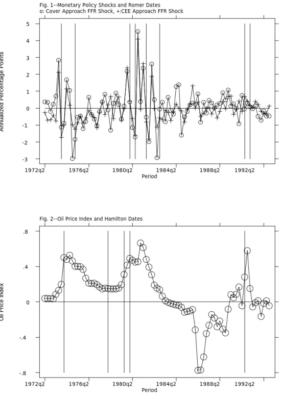
of Non-Borrowed Reserves, and T R is the log of Total Reserves. We compare our shocks with the shocks identi…ed by Garibaldi (1997), who follows Cover (1992) and get a correlation coe¢ cient of 0.82 (see Figure 1). Our results, discussed in the next section, based on Ft are, in this sense, robust to the identi…cation scheme.
3.2.2 Narrative Approach
We follow Romer and Romer (1997) who, from their reading of history, identify dates when the Federal Reserve deliberately pursued a desin‡ationary course of action.
To investigate the dynamic productivity e¤ects of contractionary monetary policy shocks iden-ti…ed via the narrative approach we estimate the following equation:
tf pit= ai;0+ ai;1 t + 8 X j=1 bi;jrrt j+ 8 X j=1
ci;jtf pi;t j+ i;t
where tf pit is the log of T F Pit, and rrt is a 0/1 dummy variable that equals 1 when t equals:
1966:2, 1968:4, 1974:2, 1978:3, 1979:4, 1988:3 (Romer dates, taken from Christiano, Eichenbaum and Evans (2000), p. 60). The vertical lines in Figure 1 mark the Romer dates. Under the identifying assumption that rrtis strictly exogenous, the OLS estimates of ai, bi and ciconsistently
estimate the IRF of TFP to a Romer shock. Eight lags (quarters) of tf pit and rrt are included to
capture the dynamics of the processes.
3.3 Fiscal Policy Shocks
The extent to which movements in …scal variables re‡ect current developments in the domestic US economy depends on the de…nitions of the …scal variables. For instance, while some transfer expenditures are highly reactive to the state of the economy, innovations to defense spending are generally thought of as exogenous shocks. This observation motivates treating defense related variables separately from non-defense variables. Hence, we o¤er two methods to identify …scal policy shocks: the …rst focuses on innovations to defense spending, and draws on Rotemberg and Woodford (1992); the second addresses shocks to a broader measure of government spending (defense and non-defense) and to a revenue variable, and follows Blanchard and Perotti (2002). While focusing on military variables is certainly less demanding in terms of identifying restrictions, by using broader spending measures we are likely to uncover …scal policy shocks with larger real e¤ects. Nevertheless, each of these two approaches provides an assessment of the robustness of the results obtained under the other.
3.3.1 Defense Spending
Rotemberg and Woodford (1992) identify a policy shock to their defense spending policy variable as the residual in a regression of the form:
gt= z( t) + gt
where tis the information set available to the …scal authority when it sets its operating instrument
gt, and z is a linear policy rule. gt is the policy shock, a serially uncorrelated residual, orthogonal
to the elements of t. Under these identifying assumptions, the IRF of a variable xt to a …scal
policy shock gt is consistently estimated by regressing xt via OLS on current and lagged values of g
t.
3.3.2 Total Government Spending and Taxes
Blanchard and Perotti (2002) study the dynamic e¤ects of shocks to government spending and taxes on output by means of a structural VAR that relies on institutional information about the tax and transfer systems. The policy variables consist in one expenditure variable, total purchases of goods and services (spending), and one revenue variable, total tax revenues minus transfers (taxes). In the …rst step we estimate the structural VAR and recover the policy shocks gt (spending) and tt (tax). Then, we consistently estimate the IRF of a variable xtto the …scal policy shock yt, y = g, t,
by regressing xt via OLS on current and lagged values of yt. We also consider that contractionary
…scal shocks may have di¤erent e¤ects from expansionary …scal shocks.
3.4 Oil Shocks
Davis (1987) claims that allocative disturbances, such as oil price shocks, have more powerful real e¤ects when they reinforce, rather than reverse, the direction of past disturbances. Davis and Haltiwanger (1999) o¤er a speci…c oil price shock designed along these lines, and de…ne an oil price shock index as the log of the following ratio: the current real oil price divided by a weighted average of its observations in the prior 20 quarters, with weights that sum to one and decline linearly to zero. Interestingly, the authors report that their result is especially important for samples that extend beyond 1985, which further supports results found in Hamilton (1996). Since the TFP series used in this paper start in 1972:2 and end in 1992:4, the concerns about the appropriate oil price shock measure expressed in the above studies are of practical importance here, leading us to adopt the Davis and Haltiwanger oil price shock index (oil index) as a measure of oil price shocks.
A complementary strategy to identify oil price shocks has been followed by Hamilton (1985), who adopts a narrative approach. Hamilton isolates a set of episodes (dates) marked by sharp exogenous oil price increases. Hoover and Perez (1994) update Hamilton’s work and identify ten oil price shocks in total: {1947:4, 1953:2, 1956:2, 1957:1, 1969:1, 1970:4, 1974:1, 1978:1, 1979:3, 1981:1}. We use these dates and 1991:3 (to mark the Iraqi invasion of Kuwait) to construct a dummy variable that signals an oil price shock identi…ed via the narrative approach (oil dummy or Hamilton dates). The vertical lines in Figure 2 correspond to the Hamilton dates. Not surprisingly, the Hamilton dates tend to coincide with the onset of prolonged increases in the oil price index.
Oil Price Index We estimate the IRFs of sectoral TFPs to an innovation to the oil price index as follows: …rst, we …t an autoregressive process to the oil price index (opt), whose residuals are
de…ned as the innovations to the oil price index (eot); second, we regress the log of sectoral TFP on its own lagged values, current and lagged values of the oil index, and a deterministic trend. Finally, we simulate the regressions to compute the IRFs of TFP to eot. To be speci…c, we estimate the following equations via OLS equation by equation:
opt= ap;0+ 8 X j=1 ap;jopt j+ eot tf pit= ai;0+ ai;1 t + 8 X j=1 bi;jtf pi;t j + 8 X j=0 ci;jopt j+ ei;t
Oil Dummy We estimate the following equation:
tf pit = i;0+ i;1 t + 8 X j=1 i;jodt j+ 8 X j=1
i;jtf pi;t j+ i;t
where odt is the oil dummy. Under the identifying assumption that odt is strictly exogenous, the
OLS estimates of the parameters and consistently estimate the IRF of TFP to an oil dummy shock.
4
Results and Interpretations
4.1 Results
This section documents the e¤ects of the monetary, …scal, and oil shocks on TFP for the 20 2-digit US manufacturing industries considered. As we saw in sections 3 and 4, this study considers several speci…cations of TFP for each industry. To achieve a balance between ease of interpretation and re‡ection of the true importance of trying several TFP speci…cations we focus on the following eight
parameterizations of TFP: 'i, which relates to the importance of a procyclical labor utilization rate, taking on values f0; 0:1; 0:2; 0:3g, and i= i, the markup-returns to scale ratio, which indexes for
imperfect competition-returns to scale, taking on values f1; 1:2g. In practice, and as a general result, the greater 'i and/or i= i (loosely speaking, the greater the correction), the further away from the unshocked path is the IRF of TFP for any shock. The discussion that follows is organized by type of shock. For brevity, we focus on the typical industry and interesting exceptions. Finally, and whenever appropriate, the IRFs correspond to shocks with a size of one standard deviation and are measured as percentage deviations from the unshocked path.
Monetary Policy Shocks Part A.1 of Figure 3 displays selected IRFs of TFP and two standard-errors-bands to a contractionary federal funds rate shock, when tight and easy shocks are assumed to have symmetric e¤ects. Let’s …rst look at the typical industry, represented by the aggregate manufacturing industry. The lines with circles are the IRFs of the di¤erent TFP speci…cations tried, and the solid lines the associated two standard-errors-bands. The clustering of the lines indicates that the typical response of TFP is fairly small and insensitive to changes in 'i or in
i= i. There is a single noteworthy exception to this permissive pattern, displayed in Part A.2
of Figure 3: in Industry Machinery (SIC 35), TFP rises to level o¤ at the tenth quarter after the shock (in the 2%-3% range, depending on the speci…cation), and is accompanied by a transitory decline in output (not reported), as predicted by the Opportunity Cost View. We get the same results for a contractionary nonborrowed-reserves shock. Quite interestingly, Industry Machinery (SIC 35) was again the only industry with a signi…cant, positive TFP response at longer horizons. Note that in no industry does TFP decline after a contractionary shock, unlike learning-by-doing or capital market imperfections theories suggest.
Part A of Figure 4 presents selected responses of TFP to tight and easy federal funds rate shocks. Allowing for asymmetric e¤ects makes little di¤erence overall; responses to both tight and easy shocks tend to be statistically insigni…cant (16-20 quarters). Interestingly, the responses to tight shocks tend to be positive. The only ‡agrant cases of asymmetries occur in Industry Machinery and Equipment (SIC 35), where a tight shock leads to an increase in TFP, and an easy shock has no noticeable e¤ect; and in Food and Kindred Products (SIC 20), where an easy shock has negative productivity e¤ects, and a tight shock has no noticeable e¤ects. These asymmetries are con…rmed when we use F-tests for the presence of asymmetries in the TFP responses. Figure 7 displays the p-values of these tests. Each TFP speci…cation has an associated p-value. A simple way to summarize the multitude of tests per industry is to report the maximum and minimum p-values over all speci…cations. If both extremes are greater than we fail to reject the null of
symmetry at the con…dence level for all speci…cations considered. If the interval between the maximum and minimum p-values contains the desired con…dence level, then we need to look deeper at which speci…cations led to which results before reaching a conclusion. Fortunately, the latter situation occurred only twice, in Printing and Publishing (SIC 27) and Rubber Products (SIC 30). Clearly, the picture that emerges from these tests is one of symmetry, with the above mentioned exceptions of Industry Machinery and Equipment (SIC 35) and Food and Kindred Products (SIC 20). Finally, we obtain the same qualitative results with tight and easy non-borrowed reserves shocks.
Part B of Figure 4 displays the typical response of TFP and output (the line with crosses) to a Romer shock (estimation in log-levels). Now there are no signs of signi…cant productivity e¤ects. The same results emerge with estimation in growth rates.
Fiscal Policy Shocks Part A of Figure 5 displays the IRFs of military spending and military employment to an expansionary shock to military spending ( mt ). Part B of Figure 5 presents selected IRFs of TFP and output. Clearly, the TFP responses barely change across speci…cations. Most industries exhibit weak responses of TFP, regardless of the output response. However, in Industry Petroleum and Coal Products (SIC 29) output (temporarily) decreases and TFP increases, and in Instruments and Related Products (SIC 38), both output and TFP decrease.
Part C of Figure 5 looks at the e¤ects of an expansionary total spending shock, when tight and easy shocks are assumed to have symmetric e¤ects. Food and Kindred Products (SIC 20) is the only industry where the TFP response at 20 quarters after the shock is greater in absolute value than two standard-errors, with an expansionary spending shock leading to a decline of TFP of about -1.5%. Once more, changing the parametrization of TFP does not change the results in any substantive way. Turning to the tax shock ( tt), there is no evidence of signi…cant productivity e¤ects in any industry.
Part D of Figure 5 presents the results for tight and easy spending shocks. In many industries, a tight shock leads to an increase in TFP (16-20 quarters), although not greater than two standard-errors. Again, tax shocks have no sizable e¤ects on TFP. The two bottom panels of Figure 7 document the ubiquitous absence of asymmetries for …scal shocks. Chemicals and Allied Products (SIC 28) and Rubber and Plastics (SIC 30) for spending shocks are the exceptions, as expected, in light of their IRFs.
Oil Shocks The …rst panel of Figure 6 displays the response of the oil price index to an own shock. The other panels display selected responses of output and TFP (estimation in log-levels).
The typical TFP response is one of virtually no impact response, followed by very mild changes and quick reversion to zero. There is a single exception to this pattern: in Food Products (SIC 20), TFP steadily rises up to 2%-3%, and is associated with a transitory decrease in output.
The results using the oil dummy are remarkably similar. In particular, the e¤ect in Food Products (SIC 20) is again 2%-3%, and is accompanied by a transitory decline in output. However, now Petroleum and Coal Products (SIC 29) shows a decline in TFP. On balance, the typical industry shows virtually no response of TFP, with the clear exception being a positive e¤ect in Food Products (SIC 20).
4.2 Interpretations
Summary of Results and Interpretations The variation in the results brought about by the di¤erent speci…cations of TFP is small. Ditto, the evidence speaks in favor of very small productivity e¤ects of monetary, …scal, and oil shocks. Table 2 contains the pairs of industries and shocks where signi…cant TFP e¤ects (20 quarters after the shock) were found. The large majority of the cells (read industries-shocks pairs) show contractionary shocks having positive productivity e¤ects, in accordance with the Opportunity Cost View. Furthermore, in two other instances, expansionary shocks have negative e¤ects, as predicted by a symmetric version of the Opportunity Cost View. When do contractionary (expansionary) shocks have negative (positive) productivity e¤ects, as predicted by learning-by-doing and capital market imperfections theories? Only Petroleum and Coal Products (SIC 29) and Chemicals and Allied Products (SIC 28) show such a pattern (for military spending and oil shocks, and total spending shocks, respectively). Table 2 also reveals the presence of asymmetries, although in a localized manner. Note also that contractionary oil shocks cause TFP to decline only in Petroleum and Coal Products (SIC 29).
Note that the identi…ed shocks do help explain activity and hence are suitable for the quanti…-cation of the importance of the Opportunity Cost View and competing theories. Figure 8 displays p-values of F-tests of exclusion of military purchases, oil price index, oil dummy, and Romer dummy in univariate regressions models of sectoral industrial output, job creation, and job destruction (with the last two series taken from Davis et al. (1996)). The variation in the results does not blur the main point taken from Figure 8: the signal extracted with the identi…ed shocks is in most cases strong enough for our purposes. In addition, Figure 9 shows that in many instances the shocks help explain the TFP indices.
The Role of Job Reallocation Aghion and Howitt (1998, Ch. 8) and Aghion and Saint-Paul (1998) allude to the work by Hall (1991) as the …rst formalization of the ideas embodied in the
Opportunity Cost View. According to Hall: “Measured output may be low during (downturn) periods, but the time spent reorganizing pays o¤ in its contribution to future productivity.” Hall claims that there is relatively more reorganization going on during downturns than in upturns, based on the fact job reallocation for the US manufacturing sector is countercyclical (Davis and Haltiwanger (1992)). The countercyclicality of job reallocation is also mentioned by Aghion and Saint-Paul (1998), and Aghion and Howitt (1998, Ch. 8) as evidence supportive of the Opportunity Cost View. By the same token, Hall and Taylor (1996, p. 136) note in their macroeconomics textbook that the large amount of job reallocation typical of downturns may be the “silver lining to the storm clouds of recessions.”
Based on the above mentioned studies, we investigate the role of job reallocation as a channel linking the considered shocks and productivity growth. If the contractionary shocks lead to higher productivity growth but not to higher job reallocation, we interpret the evidence as speaking against the empirical importance of job reallocation as a productivity improving activity. Conversely, if the contractionary shocks lead to higher productivity and to higher job reallocation, we do not dismiss the thesis that job reallocation may play a signi…cant role in the relationship between the shocks and productivity change.
We use data described in Davis et al. (1996) to construct sectoral measures of job reallocation and estimate the impact that the monetary, …scal, and oil shocks have on job reallocation using the methods employed in the estimation of the IRFs. Table 3 presents the cumulative responses of job reallocation to contractionary monetary, …scal, and oil shocks. In all six cases where Opportunity Cost View e¤ects were found (see Table 2) the cumulative response of job reallocation is positive at the twelfth period after the shock. Furthermore, the responses are substantially higher than the response of the average industry. Taken at face value, these results suggest that job reallocation may be at play and may help explain the observed Opportunity Cost View e¤ects.
The Role of the Real Interest Rate As discussed in the introduction, the smaller the increase in the real interest rate, the more productivity should increase for a given transitory decline in demand. Turning to an empirical application of this result, what is the evidence for the several shocks considered? While it is agreed that transitory contractionary monetary shocks lead to a transitory increase in the real interest rate (Christiano, Eichenbaum and Evans (2000)), the empirical evidence on transitory contractionary spending shocks supports both temporary declines in the real interest rate and no signi…cant e¤ects (Karayalçin (1999)). Now recall that four out of the six Opportunity Cost View cases were found for contractionary spending shocks, which seems to agree with the Opportunity Cost View. Of course, in light of the reduced number of signi…cant
TFP responses, we should interpret these results as suggestive, but hardly de…nitive.
5
Final Remarks
The typical 2-digit SIC US manufacturing industry shows small productivity e¤ects in response to monetary policy, …scal policy, and oil shocks. However, there are exceptions to this pattern. Interestingly, the exceptions are generally characterized by temporary contractionary policy shocks having positive productivity e¤ects (16-20 quarters), suggesting that there is signi…cant investment in productivity going on during transitory downturns. In addition, there are signs of asymmetries in the responses of productivity, with productivity responses to contractionary policy shocks being, in general, positive and larger than their counterparts to expansionary shocks. Overall, the evidence lends very little support to learning-by-doing and capital market imperfections theories. These results are robust to the alternative speci…cations of TFP and identifying strategies employed in the empirical framework, that take stock on the sate-of-art in the relevant literature. The data do not dismiss the thesis that job reallocation and the real interest rate may be important channels linking the considered shocks and productivity growth. As for policy implications, the data reveal that contractionary policy shocks do not lead to declines in productivity both at the industry level and at the aggregate manufacturing level.
References
[1] Aghion, P., Howitt, P., 1998. Endogenous Growth. MIT Press.
[2] Aghion, P., Saint-Paul, G., 1991. On the virtues of bad times: an analysis of the interaction between economic ‡uctuations and productivity growth. CEPR Discussion Paper 578.
[3] Aghion, P., Saint-Paul, G., 1998. Virtues of bad times: interaction between productivity growth and economic ‡uctuations. Macroeconomic Dynamics 2, 322-344.
[4] Basu, S., Fernald, J., Kimball, M., 1999. Why is productivity procyclical? Why do we care? Board of Governors of the Federal Reserve System, IFDP 638.
[5] Burnside, C., Eichenbaum, M., Rebelo, S., 1995. Capital utilization and returns to scale. NBER Macroeconomics Annual.
[6] Christiano, L., Eichenbaum, M., Evans, C., 2000. Monetary policy shocks: what have we learned and to what end?, in Taylor and Woodford, Handbook of Macroeconomics.
[7] Cover, J., 1992. Asymmetric e¤ects of positive and negative money-supply shocks. Quarterly Journal of Economics 107(4), 1262-1282.
[8] Davis, S., 1987. Allocative disturbances and speci…c capital in real business cycle theories. American Economic Review 77(2), p 326-332.
[9] Davis, S., Haltiwanger, J., 1992. Gross job creation, gross job destruction, and employment reallocation. Quarterly Journal of Economics 107(3), p 819-863.
[10] Davis, S., Haltiwanger, J., 1999. Sectoral job creation and job destruction responses to oil price changes. NBER Working Paper 7095.
[11] Davis, S., Haltiwanger, J., Schuh, S., 1996. Job creation and job destruction. MIT Press.
[12] Evans, C., 1992. Productivity shocks and real business cycles. Journal of Monetary Economics 29(2), p 191-208.
[13] Fay, J., Medo¤, J., 1985. Labor and output over the business cycle: some direct evidence. American Economic Review 75(4), p 638-655.
[14] Gali, J, and Hammour, M., 1992. Long-run e¤ects of business cycles. Mimeo, Columbia Uni-versity.
[15] Garibaldi, P., 1997. The asymmetric e¤ects of monetary policy on job creation and destruction. International Monetary Fund Sta¤ Papers 44(4), p 557-584.
[16] Gordon, R., 1990. Are procyclical productivity ‡uctuations a …gment of measurement error? Mimeo, Northwestern University.
[17] Hall, R., 1990. Invariance properties of Solow’s productivity residual. In P. Diamond (ed.) Productivity and Unemployment, MIT Press.
[18] Hall, R., 1991. Labor demand, labor supply, and employment volatility. In NBER Macroeco-nomics Annual, Blanchard, O., Fisher, S., eds., p 17-47 MIT Press.
[19] Hall, R., Taylor, J., 1996. Macroeconomics: theory performance and policy. W. Norton, 5th ed.
[20] Hamilton, J., 1985. Historical causes of postwar oil shocks and recessions. Energy Journal 6(1), p 97-116.
[21] Hamilton, J., 1996. This is what happened to the oil price-macroeconomy relationship. Journal of Monetary Economics 38(2), p 215-220.
[22] Hoover, K., Perez, S., 1994. Post hoc ergo propter hoc once more: an evaluation of ”does monetary policy matter” in the spirit of James Tobin. Journal of Monetary Economics 34(1), p 47-73.
[23] Jorgenson, D., Gollop, F., Fraumeni, B., 1987. Productivity and US economic growth. Harvard Economic Studies, vol. 159, Cambridge, Mass.: Harvard University Press.
[24] Karayalçin, C., 1999. Temporary and permanent government spending in a small open econ-omy. Journal of Monetary Economics 43(1), p 125-142.
[25] King, R., Rebelo, S., 2000. Resuscitating real business, in Taylor and Woodford, Handbook of Macroeconomics.
[26] Menezes, A. (2004). On the e¤ects of economic ‡uctuations on productivity growth. Mimeo, University of the Azores.
[27] Perotti, R., Blanchard, O., 2002. An empirical investigation on the dynamic e¤ects of shocks to spending and taxes on output. Quarterly Journal of Economics 117-4, p 1329-1368.
[28] Romer, C., Romer, D., 1997. Identi…cation and narrative information: a reply. Journal of Monetary Economics 40(3) p 659-665.
[29] Rotemberg, J., Woodford, M, 1992. Ologopolistic pricing and the e¤ects of aggregate demand on economic activity. Journal of Political Economy 100(6), p 1153-1207.
[30] Saint-Paul, G., 1993. Productivity growth and the structure of the business cycle. European Economic Review 37(4), p 861-883.
[31] Shapiro, M., 1996. Macroeconomic implications of variation in the workweek of capital. Brook-ing Papers on Economic Activity 2, p 79-119.
[32] Stadler, G., 1990. Business cycles models with endogenous technology. American Economic Review 80(4), p 763-778.
6
Appendix - Data
Unless otherwise mentioned, the data come from FRED. All data mentioned in this section, with the exception of the labor shares series, are seasonally adjusted, and quarterly values correspond to averages of underlying monthly data. The labor input series are the product of two (Citibase) series: total hours worked by production workers (LPHR) and total number of production workers (LPP). Growth rates of e¤ective capital services are assumed to equal growth rates of industrial electricity consumption, measured as the kilowatts of electricity used at the 2-digit SIC level, obtained from the Board of Governors. Manufacturing measures of output at the 2-digit SIC level were constructed from the Board of Governors industrial production indices. Labor shares series were taken from an updated version of the Jorgenson et al. (1987) dataset maintained by John Fernald. Since the original labor shares are available at annual frequency, it is assumed that there is no variation in these series within the year in order to obtain quarterly values. The values corresponding to the years 1990-1992 are assumed to equal the values of the year 1989.
SIC Code Industry Group 20 Food and Kindred Products Nondurable
21 Tobacco Products Nondurable
22 Textile Mill Production Nondurable 23 Apparel and Other Textiles Nondurable 24 Lumber and Wood Products Durable 25 Furniture and Fixtures Durable 26 Paper and Allied Products Nondurable 27 Printing and Publishing Nondurable 28 Chemicals and Allied Products Nondurable
29 Petroleum and Coal Products Nondurable 30 Rubber and Plastic Products Durable 31 Leather and Leather Products Nondurable 32 Stone, Clay, and Glass Products Durable
33 Primary Metals Durable
34 Fabricated Metals Durable
35 Industry Machinery and Equipment Durable 36 Electronics and Other Electrical Equipment Durable 37 Transportation Equipment Durable 38 Instruments and Related Products Durable 39 Miscellaneous Manufacturing Industries Durable
Industry Period 8 Period 12 Period 8 Period 12 Period 8 Period 12 Period 8 Period 12 20 -1.95 -2.91 -1.95 3.67 0.36 0.63 2.83 2.75 21 -1.28 -3.13 -1.28 3.40 2.48 2.52 -4.83 -5.22 22 0.04 -0.62 0.04 0.28 0.00 0.12 -1.17 -1.31 23 -0.34 -0.90 -0.34 -0.20 1.93 2.33 -2.75 -2.00 24 -0.32 -0.80 -0.32 2.18 0.02 0.49 5.51 6.36 25 -0.17 -0.68 -0.17 0.26 0.82 0.84 -0.76 0.69 26 -0.09 -0.78 -0.09 0.77 0.64 1.00 0.69 -0.18 27 0.08 -0.46 0.08 -0.15 0.65 0.77 -2.20 -1.99 28 -0.55 -0.83 -0.55 0.62 0.46 0.64 0.31 0.36 29 2.41 1.95 2.41 0.63 -1.42 -0.83 11.73 13.00 30 -0.02 -0.39 -0.02 1.77 0.03 0.52 3.22 3.12 31 -0.07 -1.08 -0.07 -1.25 -0.04 0.07 -0.48 -0.64 32 0.46 0.17 0.46 0.38 -0.94 -0.59 2.49 3.56 33 1.28 1.55 1.28 0.66 -1.84 -0.89 7.30 8.68 34 0.19 0.07 0.19 1.75 -0.18 0.24 4.94 5.62 35 0.51 0.72 0.51 0.12 -0.46 0.24 3.36 5.47 36 0.17 -0.31 0.17 0.44 0.04 0.22 0.06 1.03 37 1.27 1.20 1.27 4.08 0.28 1.37 15.29 12.88 38 -0.33 -0.81 -0.33 0.31 1.06 1.53 -0.71 0.02 39 -0.87 -2.00 -0.87 0.75 1.32 1.39 -3.14 -3.33 Average 0.02 -0.50 0.02 1.02 0.26 0.63 2.08 2.45 Comments:
Cells contain the cumulative response of job reallocation eight and twelve periods after the shocks. Values are percentage deviations from unshocked path.
Except the Oil Dummy, shocks are of a size of one standard deviation.
Table 3
FFR Monetary Shock Total Spending Shock Military Spending Shock Oil Dummy
Fig. 1--Monetary Policy Shocks and Romer Dates o: Cover Approach FFR Shock, +:CEE Approach FFR Shock
Period 1972q2 1976q2 1980q2 1984q2 1988q2 1992q2 -3 -2 -1 0 1 2 3 4 5
Fig. 2--Oil Price Index and Hamilton Dates
Period 1972q2 1976q2 1980q2 1984q2 1988q2 1992q2 -.8 -.4 0 .4 .8
o: DRFs of Different TFP Specifications; -: Two Standard-Errors-Bands Contractionary CEE FFR Shock--Symmetric Framework
Figure 3 Part A.1--Manufacturing Industry, Contractionary FFR ShockPeriods After Shock
0 4 8 12 16 20 -.03 -.02 -.01 0 .01 .02 .03
o: DRFs of Different TFP Specifications; -: Two Standard-Errors-Bands Contractionary CEE FFR Shock--Symmetric Framework
Figure 3 Part A.2--Industry Machinery, Contractionary FFR ShockPeriods After Shock
0 4 8 12 16 20 -.02 -.01 0 .01 .02 .03 .04 .05
o: DRFs of Different TFP Specifications; -: Two Standard-Errors-Bands Contractionary CEE NBR Shock--Symmetric Framework
Figure 3 Part B.1--Manufacturing Industry, Contractionary NBR ShockPeriods After Shock
0 4 8 12 16 20 -.03 -.02 -.01 0 .01 .02 .03
o: DRFs of Different TFP Specifications; -: Two Standard-Errors-Bands Contractionary CEE NBR Shock--Symmetric Framework
Figure 3 Part B.2--Industry Machinery, Contractionary NBR ShockPeriods After Shock
0 4 8 12 16 20 -.02 -.01 0 .01 .02 .03 .04 .05 .06 .07 .08 .09
o: DRFs of Different TFP Specifications; -: Two Standard-Errors-Bands Contractionary CEE FFR Shock--Asymmetric Framework
Fig. 4.A--Manufacturing, Contractionary FFR ShockPeriods After Shock
0 4 8 12 16 20 -.04 -.02 0 .02 .04 .06 .08
o: DRFs of Different TFP Specifications; -: Two Standard-Errors-Bands Expansionary CEE FFR Shock--Asymmetric Framework
Fig. 4.A--Manufacturing, Expansionary FFR ShockPeriods After Shock
0 4 8 12 16 20 -.04 -.02 0 .02 .04 .06 .08
o: DRFs of Different TFP Specifications; -: Two Standard-Errors-Bands Contractionary CEE FFR Shock--Asymmetric Framework
Fig. 4.A--Machinery, Contractionary FFR ShockPeriods After Shock
0 4 8 12 16 20 -.04 -.02 0 .02 .04 .06 .08
o: DRFs of Different TFP Specifications; -: Two Standard-Errors-Bands Expansionary CEE FFR Shock--Asymmetric Framework
Fig. 4.A--Machinery, Expansionary FFR ShockPeriods After Shock
0 4 8 12 16 20 -.04 -.02 0 .02 .04 .06 .08
o: DRFs of Different TFP Specifications; -: Two Standard-Errors-Bands Contractionary CEE FFR Shock--Asymmetric Framework
Fig. 4.A--Food, Contractionary FFR ShockPeriods After Shock
0 4 8 12 16 20 -.04 -.02 0 .02 .04 .06 .08
o: DRFs of Different TFP Specifications; -: Two Standard-Errors-Bands Expansionary CEE FFR Shock--Asymmetric Framework
Fig. 4.A--Food, Expansionary FFR ShockPeriods After Shock
0 4 8 12 16 20 -.04 -.02 0 .02 .04 .06 .08
+=Industrial Production, o=Different TFP Specifications
Figure 4 Part B--Manufacturing Industry, Romer DummyPeriods After Shock
0 4 8 12 16 20 24 -.1 -.08 -.06 -.04 -.02 0 .02 .04 .06 .08 .1
Figure 5 Part A--Military Variables, Military Spending ShockPeriods After Shock
Military Purchases Military Employment
0 4 8 12 16 20 24 -.01 0 .01 .02 .03 .04
.05 +=Industrial Production, o=Different TFP Specifications
Figure 5 Part B--Manufacturing Industry, Military Spending ShockPeriods After Shock
0 4 8 12 16 20 24 -.04 -.02 0 .02 .04
+=Industrial Production, o=Different TFP Specifications
Figure 5 Part B--Petroleum and Coal, Military Spending ShockPeriods After Shock
0 4 8 12 16 20 24 -.04 -.02 0 .02 .04
+=Industrial Production, o=Different TFP Specifications
Figure 5 Part B--Instruments, Military Spending ShockPeriods After Shock
0 4 8 12 16 20 24 -.04 -.02 0 .02 .04
o: DRFs of Different TFP Specifications; -: Two Standard-Errors-Bands Expansionary Total Spending Shock--Symmetric Framework
Fig. 5.C--Manufacturing, Expansionary Spending ShockPeriods After Shock
0 4 8 12 16 20 -.03 -.02 -.01 0 .01 .02 .03
o: DRFs of Different TFP Specifications; -: Two Standard-Errors-Bands Expansionary Total Spending Shock--Symmetric Framework
Fig. 5.C--Food, Expansionary Spending ShockPeriods After Shock
0 4 8 12 16 20 -.02 -.01 0 .01 .02 .03 .04 .05
o: DRFs of Different TFP Specifications; -: Two Standard-Errors-Bands Contractionary Tax Shock--Symmetric Framework
Fig. 5.C--Manufacturing, Contractionary Tax ShockPeriods After Shock
0 4 8 12 16 20 -.03 -.02 -.01 0 .01 .02 .03
o: DRFs of Different TFP Specifications; -: Two Standard-Errors-Bands Contractionary Total Spending Shock--Asymmetric Framework
Fig. 5.D--Manufacturing, Contractionary Spending ShockPeriods After Shock
0 4 8 12 16 20 -.04 -.02 0 .02 .04 .06 .08
o: DRFs of Different TFP Specifications; -: Two Standard-Errors-Bands Contractionary Total Spending Shock--Asymmetric Framework
Fig. 5.D--Manufacturing, Contractionary Spending ShockPeriods After Shock
0 4 8 12 16 20 -.04 -.02 0 .02 .04 .06 .08
o: DRFs of Different TFP Specifications; -: Two Standard-Errors-Bands Contractionary Total Spending Shock--Asymmetric Framework
Fig. 5.D--Textille, Contractionary Spending ShockPeriods After Shock
0 4 8 12 16 20 -.04 -.02 0 .02 .04 .06 .08
o: DRFs of Different TFP Specifications; -: Two Standard-Errors-Bands Contractionary Total Spending Shock--Asymmetric Framework
Fig. 5.D--Textille, Contractionary Spending ShockPeriods After Shock
0 4 8 12 16 20 -.04 -.02 0 .02 .04 .06 .08
o: DRFs of Different TFP Specifications; -: Two Standard-Errors-Bands Contractionary Total Spending Shock--Asymmetric Framework
Fig. 5.D--Chemicals, Contractionary Spending ShockPeriods After Shock
0 4 8 12 16 20 -.04 -.02 0 .02 .04 .06 .08
o: DRFs of Different TFP Specifications; -: Two Standard-Errors-Bands Contractionary Total Spending Shock--Asymmetric Framework
Fig. 5.D--Chemicals, Contractionary Spending ShockPeriods After Shock
0 4 8 12 16 20 -.04 -.02 0 .02 .04 .06 .08
o: DRFs of Different TFP Specifications; -: Two Standard-Errors-Bands Contractionary Total Spending Shock--Asymmetric Framework
Fig. 5.D--Rubber, Contractionary Spending ShockPeriods After Shock
0 4 8 12 16 20 -.04 -.02 0 .02 .04 .06 .08
o: DRFs of Different TFP Specifications; -: Two Standard-Errors-Bands Contractionary Total Spending Shock--Asymmetric Framework
Fig. 5.D--Rubber, Contractionary Spending ShockPeriods After Shock
0 4 8 12 16 20 -.04 -.02 0 .02 .04 .06 .08
DRF of Oil Price Index To Own InnovationPeriods After Shock
0 4 8 12 16 20 24 -.2
0
1.3 +=Industrial Production, o=Different TFP Specifications
Fig. 6--Manufacturing, Oil Price Index Shockper
0 4 8 12 16 20 24 -.08 -.06 -.04 -.02 0 .02 .04 .06 .08
+=Industrial Production, o=Different TFP Specifications
Fig. 6--Food, Oil Price Index Shockper
0 4 8 12 16 20 24 -.08 -.06 -.04 -.02 0 .02 .04 .06 .08
+=Industrial Production, o=Different TFP Specifications
Fig. 6--Petroleum, Oil Dummy ShockPeriods After Shock
0 4 8 12 16 20 24 -.14 -.1 -.06 -.02 .02 .06 .1 .14
Maximum and Minimum p-values of F-tests over all TFP specifications Ho: Long-Run TFP response to Tight=Long-Run TFP response to Easy
Industry SIC Code
20 21 22 23 24 25 26 27 28 29 30 31 32 33 34 35 36 37 38 39 0
.05 .1 1
Maximum and Minimum p-values of F-tests over all TFP specifications Ho: Long-Run TFP response to Tight=Long-Run TFP response to Easy
Industry SIC Code
20 21 22 23 24 25 26 27 28 29 30 31 32 33 34 35 36 37 38 39 0
.05 .1 1
Maximum and Minimum p-values of F-tests over all TFP specifications Ho: Long-Run TFP response to Tight=Long-Run TFP response to Easy
Industry SIC Code
20 21 22 23 24 25 26 27 28 29 30 31 32 33 34 35 36 37 38 39 0
.05 .1 1
Ho: Variables do not Granger cause Industrial Production D--Oil Dummy, I--Oil Index, R--Romer Dummy, M--Military Shock
Industry SIC Code
20 21 22 23 24 25 26 27 28 29 30 31 32 33 34 35 36 37 38 39 .05 .1 1 D D D D D D D D D D D D D D D D D D D D I I I I I I I I I I I I I I I I I I I I R R R R R R R R R R R R R R R R R R R R M M M M M M M M M M M M M M M M M M M M
Ho: Variables do not Granger cause Job Creation
D--Oil Dummy, I--Oil Index, R--Romer Dummy, M--Military Shock
Industry SIC Code
20 21 22 23 24 25 26 27 28 29 30 31 32 33 34 35 36 37 38 39 .05 .1 1 D D D D D D D D D D D D D D D D D D D D I I I I I I I I I I I I I I I I I I I I R R R R R R R R R R R R R R R R R R R R M M M M M M M M M M M M M M M M M M M M
Ho: Variables do not Granger cause Job Destruction
D--Oil Dummy, I--Oil Index, R--Romer Dummy, M--Military Shock
Industry SIC Code
20 21 22 23 24 25 26 27 28 29 30 31 32 33 34 35 36 37 38 39 .05 .1 1 D D D D D D D D D D D D D D D D D D D D I I I I I I I I I I I I I I I I I I I I R R R R R R R R R R R R R R R R R R R R M M M M M M M M M M M M M M M M M M M M
Maximum and Minimum p-values of F-tests over all TFP specifications Ho: Romer Dummy does not Granger cause TFP
Industry SIC Code
20 21 22 23 24 25 26 27 28 29 30 31 32 33 34 35 36 37 38 39 0
.05 .1
1
Maximum and Minimum p-values of F-tests over all TFP specifications Ho: Military Spending does not Granger cause TFP
Industry SIC Code
20 21 22 23 24 25 26 27 28 29 30 31 32 33 34 35 36 37 38 39 0
.05 .1
1
Maximum and Minimum p-values of F-tests over all TFP specifications Ho: Oil Price Index does not Granger cause TFP
Industry SIC Code
20 21 22 23 24 25 26 27 28 29 30 31 32 33 34 35 36 37 38 39 0
.05.1 1
Maximum and Minimum p-values of F-tests over all TFP specifications Ho: Oil Dummy does not Granger cause TFP
Industry SIC Code
20 21 22 23 24 25 26 27 28 29 30 31 32 33 34 35 36 37 38 39 0
.05.1 1