School of Economics and Management

Carlos Pestana Barros & Nicolas Peypoch

A Comparative Analysis of Productivity Change in Italian and

Portuguese Airports

WP 006/2007/DE

_________________________________________________________

Sandra Gomes & Catarina Mendicino

Housing Market Dynamics: Any News?

WP 23/2012/DE

_________________________________________________________

De p a rtm e nt o f Ec o no m ic s

W

P

ISSN Nº 0874-4548

School of Economics and Management

Housing Market Dynamics: Any News?

Sandra Gomesy

Bank of Portugal

and ISEG/TULisbon

Caterina Mendicinoz

Bank of Portugal

July 2012

Abstract

This paper quanti…es the importance of news shocks for housing market ‡uctuations. To

this purpose, we extend Iacoviello and Neri (2010)’s model of the housing market to include

news shocks and estimate it using Bayesian methods and U.S. data. We …nd that news shocks:

(1) account for a sizable fraction of the variability in house prices and other macroeconomic

variables over the business cycle and (2) signi…cantly contributed to booms and busts episodes

in house prices over the last three decades. By linking news shocks to agents’ expectations, we

…nd that house price growth was positively related to in‡ation expectations during the boom of

the late 1970’s while it was negatively related to interest rate expectations during the housing

boom that peaked in the mid-2000’s.

Keywords: bayesian estimation, news shocks, local identi…cation, housing market, …nancial

frictions, in‡ation and interest rate expectations.

JEL codes: C50, E32, E44.

The opinions expressed in this article are the sole responsibility of the authors and do not necessarily re‡ect the position of the Banco de Portugal or the Eurosystem. We are grateful to Paulo Brito, Nikolay Iskrev, Andrea Pescatori, Virginia Queijo von Heideken, Paolo Surico and seminar participants at the Banco de Portugal, the 2011 International Conference on Computing in Economics and Finance and ISEG/TULisbon (School of Economics and Management/Technical University of Lisbon) for useful comments and suggestions.

y_{Address: Bank of Portugal, Economic Research Department, Av. Almirante Reis 71, 1150-012 Lisbon, Portugal;} e-mail: sandra.cristina.gomes@bportugal.pt

1

Introduction

How important are expectation-driven cycles for housing market dynamics? Survey evidence shows that house price dynamics are signi…cantly related to macroeconomic expectations and particularly to optimism about future house prices appreciation.1 However, macroeconomic models of the housing market mainly rely on fundamental developments in the economy to explain ‡uctuations in house prices and residential investment. Among others, Davis and Heathcote (2005) develop a multi-sector model of the housing market that matches the co-movement of residential investment with GDP and other components of GDP by assuming technology shocks as the only source of ‡uctuations; Iacoviello and Neri (2010) add real, nominal, and credit frictions, along with a larger set of shocks, to the multi-sector framework and highlight the role of housing preference shock, technology and monetary factors.2

This paper evaluates the empirical importance of expectations-driven cycles for housing market ‡uctuations. In particular, following most of the literature on expectations-driven cycles, we explore the importance of news shocks as relevant sources of uncertainty.3 To this purpose we estimate Iacoviello and Neri (2010)’s model extended to incorporate news over di¤erent time horizons about the structural shocks of the model. The framework we use is particularly relevant to the purpose of this paper since its rich modelling structure allows for the quantifying of news shocks originated in di¤erent sectors of the economy, e.g., the housing market, the production sector, in‡ationary factors and the conduct of monetary policy. As in Schmitt-Grohe and Uribe (2012), we assume that the structural shocks of the model feature a standard unanticipated component and an anticipated component driven by innovations announced 4 and 8 quarters in advance. Thus, the innovation announced 4 quarters in advance can be views as a revision of the innovation announced 8 quarters in advance and the current innovation can be interpreted as a revision to the sum of the anticipated innovations. To quantify the empirical relevance of news shocks, we …t the model to U.S. data using likelihood-based Bayesian methods. As highlighted by Schmitt-Grohe and Uribe (2012), it is feasible to identify and estimate news shocks by using DSGE models with forward looking agents and likelihood-based methods.

This paper provides several insightful results. First, the model that allows for news shocks is

1_{In particular, Case and Shiller (2003) document that expectations of future house price increases had a role in}

past housing booms in the U.S.; Piazzesi and Schneider (2009) use the University of Michigan Survey of Consumers to show that during the boom that peaked in the mid-2000’s, expectations of rising house prices signi…cantly increased; Nofsinger (2011) argues that the emotions and psychological biases of households play an important role in economic booms.

2_{For other papers of the housing market, see, among others, Aoki, Proudman, and Vlieghe (2004), Iacoviello}

(2005), Finocchiaro and Queijo von Heideken (2009), Kiyotaki, Michaelides, and Nikolov (2010), Liu, Zha and Wang (2011).

3_{See, among others, Beaudry and Portier (2004, 2007), Floden (2007), Christiano, Ilut, Motto, and Rostagno}

strongly preferred in terms of overall goodness of …t. In particular, the data favor the inclusion of news shocks over a longer time-horizon, i.e. 8 quarters in advance. Further, on the bases of local identi…cation analysis as in Iskrev (2010a, 2010b), we argue that news shocks are neither "nearly irrelevant", i.e. do not a¤ect the solution of the model or the model implied moments, or "nearly redundant", i.e. their e¤ect can be replicated by other shocks. News shocks are distinguishable from unanticipated shocks in terms of the solution of the model and are also important in determining the statistical properties of the model. Indeed, news shocks a¤ect economic choices and, in particular, the housing and credit decisions of households di¤erently than unanticipated shocks.

Second, news shocks explain around 40 percent of business cycle ‡uctuations in house prices and a sizable fraction of variations in consumption, residential and non-residential investment. In particular, expectations about future cost-push shocks are the largest contributors to business cycle ‡uctuations. Among other news shocks, news related to productivity explains almost one-quarter of the variability in business investment. News shocks related to monetary factors account for a larger fraction of variations in house prices and consumption than expectations about future productivity shocks. A plausible reason for the importance of news shocks is related to the fact that these shocks generate the co-movement among business investment, consumption and house prices observed in the data, especially during periods of housing booms.

Third, news shocks contribute to the boom-phases in house prices, whereas the busts are al-most entirely the result of unanticipated monetary policy and productivity shocks. In particular, expectations of cost-push shocks are found to be important for the run up in house prices and residential investment during the housing booms that occurred concurrently with the energy crises of the 1970’s. Investment speci…c news shocks are the main contributor to residential investment growth during the "new economy" cycle of the late 1990’s. Expectations of housing productivity shocks and investment speci…c shocks somewhat contribute to changes in house prices during the latest boom, whereas expected downward cost pressures on in‡ation muted its increase over the same period.

the latter shock is plausibly related to the GDP growth component of the interest-rate rule followed by the monetary authority.

Further, using survey-based expectations on in‡ation and interest rates, we also test the plaus-ibility of the expectation channel featured by the model. On the base of Granger causality tests we …nd that news shocks also contain statistically signi…cant information for survey-based in‡ation and interest rate expectations. As a result, the model mimics particularly well the evidence that higher in‡ation expectations are strongly related to house prices during the boom of the 1970’s whereas lower interest rate expectations are signi…cantly related to the run up in house prices during the latest boom. The link between interest rate expectations and house prices over the last decade seems to be mainly driven by the systematic component of the policy rule, and, in particular, by expectations about GDP growth as opposed to news on monetary policy shocks.

This paper is related to the growing empirical literature that explores the role of news shocks over the business cycle. Beaudry and Portier (2006) using a VAR approach showed that business cycle ‡uctuations in the data are primarily driven by changes in agents’ expectations about future technological growth. Since their seminal paper, several authors have investigated the importance of expectations-driven cycles as a source of business cycle ‡uctuations.4 _{This paper is particularly}

related to Schmitt-Grohe and Uribe (2012) that estimating a real business cycle model, docu-ment that news on future neutral productivity shocks, investdocu-ment-speci…c shocks, and governdocu-ment spending shocks account for more than two thirds of predicted aggregate ‡uctuations in postwar U.S. data. We contribute to their …ndings by documenting that news shocks are also important for housing market ‡uctuations. Moreover, di¤erently from previous papers, we assess the relat-ive importance of the unanticipated and anticipated component of the shocks in a¤ecting both the structural and statistical properties of the model. Further, we also explore the linkage between news shocks and the endogenous expectations of the model and document how expectations on in‡ation and interest rates are related to house price booms and busts.5 To the best of our knowledge, there are no other attempts to quantify the role of news shocks for housing market ‡uctuations in this strand of the business cycle literature.

Few other authors have also studied the transmission mechanism of expectations on future

4_{Among others, see, Barsky and Sims (2009), Kurmann and Otrok (2009), Fujiwara, Hirose and Shintani (2011),}

Khan and Tsoukalas (2009), Milani and Treadwell (2009), Badarinza and Margaritov (2011).

5_{Very few papers analyze the ability of DSGE models to match the dynamics of expectations. These other studies}

fundamentals to house prices in macro models. Lambertini, Mendicino and Punzi (2010) show that changes in expectations of future macroeconomic developments can generate empirically plausible boom-bust cycles in the housing market; Tomura (2010) documents that uncertainty about the duration of a period of temporary high income growth can generate housing booms in an open economy model; Adam, Kuang and Marcet (2011) explain the joint dynamics of house prices and the current account over the years 2001-2008 by relying on a model of "internally rational" agents that form beliefs about how house prices relate to economic fundamentals; Burnside, Eichenbaum and Rebelo (2011) document that heterogeneous beliefs about long-run fundamentals can lead to booms and busts in the housing market. We complement previous …ndings by providing a quantitative assessment of the importance of expectation-driven cycles for housing prices and by documenting the type of news shocks that are more relevant in driving housing market ‡uctuations. The rest of the paper is organized as follows. Section 2 describes the model and Section 3 describes the estimation methodology. Section 4 tests for local identi…cation of the shocks. Section 5 comments on the results of news shocks as a source of ‡uctuations in the housing market and Section 6 investigates the role of news shocks for booms and busts in house prices and residential investment. Section 7 relates agents’ expectations to house prices. Section 8 concludes.

2

The Model

We rely on the model of the housing market developed by Iacoviello and Neri (2010). The model features real, nominal, and …nancial frictions, as well as a large set of shocks. Three sectors of production are assumed: a non-durable goods sector, a non-residential investment sector, and a residential sector. Households di¤er in terms of their discount factor and gain utility from non-durable consumption, leisure, and housing services. In addition, housing can be used as collateral for loans. For completeness, we describe the main features of the model in the next subsections.

2.1 Households

Lenders Lenders, maximize the following lifetime utility:

Ut=Et 1 X

t=0

( tGC)tzt cln (ct "ct 1) +jtln ht t

1 +

h

(nc;t)1+ + (nh;t)1+

i1+ 1+

;

where is the discount factor (0< 0 < <1), "is the external habits parameter (0< " <1), is the inverse of the elasticity of work e¤ort with respect to the real wage ( >0), and de…nes the degree of substitution between hours worked in the two sectors ( 0). GC is the trend growth rate of real consumption and c is a scaling factor of the marginal utility of consumption. zt,jtand tare shocks to the intertemporal preferences, housing demand and labor supply, respectively, that follow AR(1) processes. Lenders decide how much to consume, ct, the amount of hours devoted to work in each sector, nc;t and nh;t, the accumulation of housing ht (priced atqt), the supply of intermediate inputs kb;t (priced at pb;t), the stock of land lt (that is priced at pl;t), and the stock of capital used in the two sectors of production, kc;t and kh;t. Lenders also choose the capital utilization rate in each sector, zc;t and zh;t (subject to a convex cost a( )). Finally, they decide on the amount of lending, bt. Loans yield a riskless (gross) nominal interest rate denoted by Rt. On the other hand, Lenders receive wage income (wc;t and wh;t are the real wages in each sector, relative to the consumption good price), income from renting capital (at the real rental rates Rc;t and Rh;t) and land (at the real rental rate Rl;t), and from supplying intermediate goods to …rms. Capital in the non-durable goods sector and in the housing sector as well as land depreciate at (quarterly) rates kc, kh and h. Finally, Lenders receive (lump-sum) dividends from owning …rms and from labor unions (Dt). Thus, their period budget constraint is:

ct+

kc;t

Ak;t

+kh;t+kb;t+qtht+pl;tlt bt=

wc;tnc;t

Xwc;t

+wh;tnh;t

Xwh;t

+

+ Rc;tzc;t+

1 kc

Ak;t

kct 1+ (Rh;tzh;t+ 1 kh)kht 1+pb;tkb;t+ (pl;t+Rl;t)lt 1+qt(1 h)ht 1

+Dt

Rt 1bt 1

t c;t h;t

a(zc;t)kc;t 1

Ak;t

a(zh;t)kh;t 1;

where t is the (quarter-on-quarter) in‡ation rate in the consumption goods sector. Ak;t is an investment-speci…c technology shock that represents the marginal cost of producing consumption good sector speci…c capital.6 _G

IKc and GIKhare the trend growth rates of capital used in the two

sectors of production and _c;t and _h;t are convex adjustment costs for capital.7

Both types of households supply labor to unions in the two sectors of production. The unions di¤erentiate labor services and sell it in a monopolistic competitive labor market. Thus, there is a wedge between the wage paid by …rms to labor unions and those received by households (Xwc;t and Xwh;t denote the markups in the non-durable and housing sectors, respectively). Wages are set according to a Calvo (1983) scheme (with a 1 w;c exogenous probability of re-optimization when labor is supplied to the non-durable goods sector union and a 1 w;h is the probability in the housing sector) with partial indexation to past in‡ation (with parameters w;c and w;h in the corresponding sectors).

Borrowers Borrowers’ and Lenders’ utility function are similarly de…ned.8 Borrowers do not own capital, land or …rms. They only receive dividends from labor unions. Hence, the borrowers period budget constraint is:

c0_t+qt h

0

t (1 h)h

0

t 1 b 0

t

w_c;t0 n0_c;t

X_wc;t0 +

w0_h;tn0_h;t

X_wh;t0 +D

0

t

Rt 1b 0

t 1

t

:

Borrowers are constrained in that they may only borrow up to a fraction of the expected present value of next-period value of their housing stock:

b0_t mEt

qt+1h 0

t t+1

Rt !

;

wherem 1 represents the loan-to-value ratio.9

2.2 Firms

Non-durable goods, business capital and housing are produced by a continuum of wholesale …rms that act under perfect competition. Price rigidities are introduced in the non-durable sector, while

7

c;t = 2G_IKckc kc;t

kc;t 1 GIKc

2 _k

c;t 1

(1+ AK)t is the good-sector capital adjustment cost, and h;t = kh

2GIKh

kh;t

kh;t 1 GIKh

2

kh;t 1is the housing-sector capital adjustment cost; AKrepresents the long-run net growth

rate of technology in business capital, kc and khare the coe¢cients for adjustment cost (i.e., the relative prices of

installing the existing capital) for capital used in the consumption sector and housing sector, respectively.

8_{Variables and parameters with a prime (}0 _{) refer to Borrowers while those without a prime refer to Lenders.}

9_{Given the assumed di¤erence in the discount factor, the borrowing restriction holds with equality in the steady}

retail sale prices of housing are assumed to be ‡exible.

Wholesale …rms Wholesale …rms operate in a perfect competition ‡exible price market and produce both non-durable goods, Yt, and new houses, IHt. To produce non-durable goods the wholesale …rms use labor (supplied by both types of households) and capital as inputs of production while the producers of new houses also use intermediate goods and land. Production technologies are assumed to be Cobb-Douglas:

Yt= Ac;t(nc;t) n

0

c;t

1 1 c

(zc;tkc;t 1) c

IHt= Ah;t(nh;t) n

0

h;t

1 1 h b l

(zh;tkh;t 1) hkb;tbltl1:

where is a parameter that measures the labor income share of Lenders and Ah;t and Ac;t are the productivity shocks to the non-durable goods sector and housing sector, respectively. The productivity shocks are de…ned as:10

ln(Ax;t) =tln(1 + Ax) + ln(Zx;t); x=c; h

whereln(Zc;t)andln(Zh;t)followAR(1)processes (with serially uncorrelated, zero mean innovations with standard-deviations Ac and Ah) and Ac and Ah are the long-run net growth rates of

technology in each sector, such that:

ln(Zx;t) = Axln(Zx;t 1) +ux;t:

Retailers Wholesale …rms in the non-durable goods sector sell their output under perfect com-petition to retailers that act under monopolistic comcom-petition when selling the goods to households. Retailers di¤erentiate the non-durable goods and then sell them to households, charging a markup,

Xt, over the wholesale price. Retailers set their prices under a Calvo-type mechanism (the exo-genous probability of re-optimization is equal to 1 ) with partial indexation to past in‡ation (driven by parameter ). This setup leads to the following forward-looking Phillips curve:

ln t ln t 1= GC(Etln t+1 ln t) ln(

Xt

X) +up;t

where = (1 )(1 ) and up;t is an i.i.d. cost-push shock.

1 0_{The investment-speci…c technology shock,A}

2.3 Monetary Policy Authority

The monetary authority sets the (gross) nominal interest rate according to the following Taylor-type rule:

Rt=RrtR1

(1 rR)r

t

As;t

GDPt

GCGDPt 1

(1 rR)rY

rr(1 rR)_u

R;t

whererr is the steady-state real interest rate,GDP is the economy’s gross domestic product,uR;t is an i.i.d. shock and As;t is a persistent shock to the central bank’s in‡ation target. Following Iacoviello and Neri (2009), GDP is de…ned as the sum of consumption and investment at constant pricesGDPt=Ct+IKt+qIHt, where q is real housing prices along the balanced growth path in terms of the price of the consumption good.

2.4 News Shocks

In the model there are seven AR(1) shocks – zt, jt, t, Ah;t, Ac;t, Ak;t and As;t – and two i.i.d. shocks: up;tanduR;t. Expectations of future macroeconomic developments are introduced as in the existing news shock literature. We assume that the error term of the shocks, with the exception of preferences ,ux;t, consists of an unanticipated component, "0x;t;and anticipated changesnquarters in advance, "n

x;t n, withn=f4;8g,

ux;t="0x;t+"4x;t 4+"8x;t 8;

where"x;t is i.i.d and x=fc; h; k; p; R; sg. Thus, at time t nagents receive a signal about future macroeconomic conditions at time t: As in Schmitt-Grohe and Uribe (2012) we assume anticip-ated changes four and eight quarters ahead. This assumption allows for revisions in expectations, e.g., "8_{x;t 8}can be revised at time t 4 (up or down, partially or completely, in the latter case

"4_{x;t 4}= "8_{x;t 8}) and"4_{x;t 4}+"8_{x;t 8} can be revised at time0(again, partially or completely, in the latter case"0_x;t= ("4_{x;t 4}+"8_{x;t 8})and ux;t= 0).

3

Estimation

3.1 Methodology

The set of structural parameters of the model describing technology, adjustment costs, price and wage rigidities, the monetary policy rule, and the shocks is estimated using Bayesian techniques. We proceed in two steps. First, we obtain the mode of the posterior distribution which summarizes information about the likelihood of the data and the priors on the parameters’ distributions by numerically maximizing the log of the posterior. We then approximate the inverse of the Hes-sian matrix evaluated at the mode. We subsequently use the random walk Metropolis-Hastings algorithm to simulate the posterior, where the covariance matrix of the proposal distribution is proportional to the inverse Hessian at the posterior mode computed in the …rst step. After check-ing for convergence, we perform statistical inference on the model’s parameters or functions of the parameters, such as second moments.11 For recent surveys of Bayesian methods, see An and Schorfheide (2007) and Fernandéz-Villaverde (2010).

In setting the parameters’ prior distributions, we follow Iacoviello and Neri (2010). In particular, we use a beta distribution for the serial correlations of the shocks, _Ax, and an inverse gamma distribution for the standard deviations of the shocks, x. In order to avoid over-weighting a

priori any of the two components of the shocks, we assume that the variance of the unanticipated innovation is equal to the sum of the variances of the anticipated components.12

0

x

2

= 4_x 2+ 8_x 2:

Introducing news shocks to the model adds 12 additional parameters. In order to make the estimation less cumbersome, we reduce the set of parameters by calibrating those that a¤ect the steady state of the model. Most of these parameters are calibrated as in Iacoviello and Neri (2010) while others are set to the mean estimated values reported in their estimates. Thus, as in most estimated DSGE models, the steady-state ratios are unchanged during the estimation. As common in the literature, we also …x the autoregressive parameters of the in‡ation targeting shock.13 See Table 1.

3.2 Data

As in Iacoviello and Neri (2010), we consider ten observables: real consumption per capita, real private business and residential …xed investment per capita, quarterly in‡ation, nominal short-term interest rate, real house prices, hours worked per capita in the consumption-good and the housing

1 1_{To perform inference we discard the …rst 10 per cent of observations.}

sectors, and the nominal wage quarterly change in the consumption and housing sector.14 _Real

variables are de‡ated by the output implicit price de‡ator in the non-farm business sector. We also allow for measurement error in hours and wage growth in the housing sector. As in Iacoviello and Neri (2010) we use quarterly data from 1965Q1. The desire to have a sample over which monetary policy was conducted using conventional tools restrict us to consider data up to 2007Q4.15

3.3 Parameter Estimates

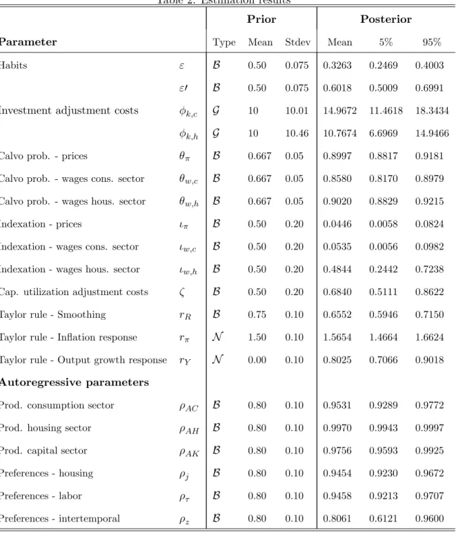
Tables 2 and 3 display the priors chosen for the model’s parameters and the standard deviations of the shocks, as well as the posterior mean, standard deviations and the 95 percent probability intervals. The posterior estimates of the model’s parameters feature a substantial degree of wage and price stickiness, and a low degree of indexation in prices and wages in the consumption sector. The estimated monetary policy rule features a moderate response to in‡ation, a modest degree of interest-rate smoothing, and a positive reaction to GDP growth. Finally, all shocks are quite persistent and moderately volatile. News shocks display a much lower volatility than unanticipated shocks.

We do not …nd sizable di¤erences with respect to the estimates reported by Iacoviello and Neri (2010). We …nd a slightly higher response to in‡ation and GDP growth and a lower response to the lagged interest rate in the Taylor Rule as well as higher stickiness and lower indexation in the Phillips Curve. These di¤erences are mainly related to revisions in the series for in‡ation.16

3.4 Overall Goodness of Fit

In order to evaluate the importance of news shocks for the overall goodness of …t of the model, we compare the estimated model presented above against two other speci…cations: without news shocks (ux;t = "0x;t) and with news only at a 4 quarter horizon (ux;t = "0x;t +"4x;t 4). The latter

speci…cation helps us to assess the potential importance of signal revisions.

Table 4 reports the log marginal data density of each model, the di¤erence with respect to the log marginal data density of the model without news shocks, and the implied Bayes factor.17 Both versions of the model that allow for news shocks display a signi…cantly higher log data density

1 4_{For details on the series used and the data transformations see the Appendix.}

1 5_{The exclusion of the most recent years allows to understand housing market dynamics over the average business}

cycle, i.e. not a¤ected by the period of extreme macroeconomic ‡uctuations that characterized the recent …nancial crisis. A version of the model with the addition of a collateral shocks has been separately estimated. However, due to the lack of data on debt and house holding of credit constraint households, we …nd it di¢cult to identify such a shock and, thus, to capture the dynamics of the recent credit crunch.

1 6_{Iacoviello and Neri (2010) used data from 1965Q1 to 2006Q4. Therefore, we use a di¤erent vintage of the data}

set.

compared to the no-news model. Accordingly, the Bayes factor indicates decisive evidence in favor of the models with news shocks, see Je¤reys (1961) and Kass and Raftery (1995). In order for the model without news to be preferred, we would need a priori probability over this model 1:7 1025

larger than the prior belief about the model with 4 and 8-quarter ahead news.18 Thus, we conclude that the data strongly favor the inclusion of news shocks. Moreover, the model that also includes longer horizon signals outperforms all other speci…cations in terms of overall goodness of …t.

All versions of the model are estimated using our updated data set. See Section 3.2. As a last check, in the last three rows of Table 4 we report the Bayes factor using Iacoviello and Neri (2010) data set. The same results hold.

4

Are News Shocks Di¤erent than Other Shocks?

In order to avoid concerns related to the identi…ability of news shocks, we test for local identi…cation in the model and in the moments. To circumvent the di¢culty of explicitly deriving the relationships between the deep parameters of the model and the structural characteristics of the model used to estimate them, we use the local identi…cation approach. As in Schmitt-Grohe and Uribe (2012) we rely on the methodology proposed by Iskrev (2010a). The analysis consists of evaluating the ranks of Jacobian and can be performed for any given system of equations describing the linearized model and the corresponding parameter space. The analysis strictly follows Iskrev (2010a and 2010b).

Let JT ( ) be the Jacobian matrix of the mapping from the deep parameters of the model, ; to the vector mT collecting the parameters that determine the unconditional theoretical moments of the observables (of sample size T) in the model. The Jacobian matrix can be factorized as

JT ( ) = @m_@ @_@ , where represents a vector collecting the (non-constant elements of the)

reduced-form parameters of the …rst-order solution to the model, @m_@ measures the sensitivity of the moments to the reduced-form parameters ; and @_@ measures the sensitivity of to the deep parameters . A parameter i is locally identi…able if the Jacobian matrix @J_@( )_i has full column rank at i.19 Evaluating the Jacobian matrix @J_@( ) analytically, we …nd that, in a neighborood of the posterior mean of the estimated parameters, all parameters reported in Tables 2 and 3 are locally identi…ed.20

A parameter is weakly identi…ed if it is "nearly irrelevant", i.e. does not a¤ect the solution of the model or the model implied moments, or it is"nearly redundant", i.e. if its e¤ect can be replicated by other parameters. For completeness, in the following, we summarize the conditions for identi…cation both in the model and in the moments.

Identi…cation in the model. Since fully characterizes the steady state and the model

1 8_{6:4 10}12 _{larger than the prior belief about the model with 4-quarter ahead news shocks.} 1 9_{We compute derivatives of the …rst and second order covariances.}

dynamics, low sensitivity to a particular parameter means that this parameter is unidenti…able in the model for purely model-related reasons, thus unrelated to the series used as observables in the estimation. If the Jacobian matrix @_@ does not have full column rank, then some of the parameters are unidenti…able in the model. Strictly speaking, a parameter i is (locally) weakly identi…ed in the model if either (1) is insensitive to changes in i, i.e. _@@ _i ' 0, or (2) if the e¤ects on of changing i can be o¤set by changing other parameters, i.e. cos _@@ _i;_@@ _i '1.

Regarding the identi…cation of the shocks, we measure collinearity between the column of the Jacobian @_@ with respect to the standard deviations of the news shocks, the standard deviation of the unanticipated shocks and the autocorrelation parameters. Panel A of Figure 1 reports the pairs of parameters with the highest value of the cosine among all possible combinations of shocks’ parameters. First, the maximum value of the cosine across possible sets of shocks’ parameters suggests weak collinearity relationships among these parameters with respect to the solution of the model. Second, the highest collinearity is generally not found among the standard deviation of the unanticipated component of the error term of a shock, _"0

x;t;and the standard deviation of the

anticipated components of the same shocks, _"4

x;t 4 and "8x;t 8. Thus, arguably, the unanticipated

and anticipated components of any shock do not play a similar role in the solution of the model. In other words, examining how the identi…cation of parameters is in‡uenced by the structural characteristics of the model, we …nd that both unanticipated and news shocks are identi…ed in the model.

Identi…cation in the moments. Parameters that are identi…able in the model could be poorly identi…ed if some of the variables are unobserved. On the other hand, it is important to notice that if a parameter does not a¤ect the solution of the model (@

@ i '0) then its value is also

irrelevant for the statistical properties of the data generated by the model (@J_@( )

i '0). Indeed, the

However, it is important to stress that no multicollinearity is found across parameters.

The relative importance of each shock in determining the model’s statistical properties for the ten observables used to estimate the model, can be used as a measure of the strength of identi…cation. Figure 2 reports the sensitivity in the moments to the shocks’ parameters at the posterior mean, i.e. the norm of columns of the Jacobian matrix, @J_@( );corresponding to each of the shocks parameters.21 _{News shocks display high sensitivity in the moments and are, thus, important}

in determining the statistical properties of the model. This is particularly true for expectations of investment speci…c shocks and changes in the in‡ation target, both 4 and 8 quarters ahead, and for 8-quarters ahead expectations of cost push shocks. Unanticipated shocks generally display lower sensitivity in the moments. Housing productivity shocks o¤er an exception.

Summarizing, all shocks are identi…ed, though with varying strength of iden…cation. News shocks appear to be distinguishable from unanticipated shocks both in terms of the solution of the model and for the determination of the model implied moments of the ten observables used in the estimation.

5

News Shocks and Housing Market Dynamics

In this section, we highlight key …ndings regarding the transmission mechanism of news shocks and quantify the role of news shocks for housing market dynamics. First, we analyze the contribution of news shocks for ‡uctuations of selected variables over the business cycle. Then, we assess their role for the observed house prices booms and busts over the sample period.

5.1 Transmission Mechanism

The transmission of news shocks relies on two distinguishable features. First, news shocks can induce optimism about future house price appreciation and generate hump-shaped dynamics in house prices that resemble the patterns observed in the data during periods of housing booms. Expectations about the occurrence of shocks that lead to an increase in house prices, such as a future monetary policy loosening, an increase in the productivity of consumption goods or a decline in the supply of houses, immediately generate beliefs of future appreciations in housing prices and fuel current housing demand. Consequently, house prices gradually rise, peak at the time in which expectations are ful…lled and, then, slowly decline towards the initial level. Thus, in contrast to standard unanticipated shocks, the peak e¤ect on prices and quantities is not immediate. Figure 3 reports the e¤ect of unanticipated and news shocks on house prices.

Second, news shocks generate the co-movement among house prices, consumption, residential-and non-residential investment, residential-and hours worked in both sectors of production observed in the data, especially during periods of housing booms.22 _{Figures 4 and 5 report, respectively, the e¤ect of}

selected unanticipated and the corresponding 8-quarters ahead news shocks on key macroeconomic variables. News shocks a¤ect economic choices and, in particular, the housing and credit decisions of households di¤erently than unanticipated shocks. As news spread, the value of housing collateral increases and the rise in house prices is, thus, coupled with an expansion in household credit and consumption. Moreover, due to limits to credit, Borrowers increase their labor supply in order to raise internal funds for housing investments. Given the presence of adjustment costs for capital, …rms start adjusting the stock of capital already at the time in which news about the occurrence of future shocks that come along with demand pressures in one of the two sectors spread. The increase in business and housing investment makes also GDP rise. For the increase in investment to be coupled with an increase in hours, wages rise. Thus, news shocks in this model generate pro-cyclicality among all relevant variables.23

5.2 Business Cycle Fluctuations

Are news shocks a relevant source of business cycle ‡uctuations? Table 5 shows the contribution of the anticipated and unanticipated components of the shocks to the unconditional variance of the observable variables at business cycle frequencies. News shocks account for slightly less than 40 percent of the variance in house prices, about 13 percent of the variance in residential investment, and more than half of the variance of consumption, business investment, and in‡ation. Expecta-tions 8-quarters ahead account for most of the variaExpecta-tions reported above. Regarding the di¤erent types of news shocks, news related to cost-push shocks are by far the most important source of ‡uctuations among the anticipated shocks. See Table 6. In particular, expectations about future cost push shocks explain slightly less than 30 percent of the variability in house prices, more than 40 percent of variations in consumption, business investment and in‡ation, and have about the same importance as news on productivity shocks for explaining residential investment. News shocks re-lated to monetary factors are mainly driven by the persistent shock to the target of the central bank and explain a bit more of variations in house prices and consumption than news of productivity shocks. News shocks about productivity in the three sectors explain almost one-quarter of the vari-ability in business investment. A plausible reason for the importance of news shocks is related to

2 2_{Lambertini, Mendicino and Punzi (2010) document that, over the last three decades, housing prices boom-bust}

cycles in the U. S. have been characterized on average by co-movement in GDP, consumption, business investment, hours worked, real wages and housing investment.

2 3_{For a detailed analysis of the transmission mechanism of these shocks in the framework presented above, see}

the fact that these shocks are able to generate co-movement among a broad set of macroeconomic variables.24 See section 5.1. Since news shocks are an important source of ‡uctuations in business investment, along with consumption and house prices they contribute to the co-movement across these variables.

Regarding the unanticipated component of the shocks, preference shocks have a considerable role in explaining house prices and residential investment. This result is mainly driven by the housing preference shock, which in the model resembles a housing demand shock. Housing preference shocks have been previously documented in the literature as an important source of co-movement between house prices and consumption in models of collateral constraints at the household level.25 However, as highlighted by Liu, Wang ans Zha (2011), in the absence of credit frictions at the …rm level, preference shocks turn out to be not very important for business investment, and thus, contribute little to the co-movement among house prices, consumption and business investment.

Monetary shocks explain a bit less than 10 percent of the variability in house prices and invest-ment, and about 14 percent of the volatility of the other variables whereas, productivity shocks explain around 30 and 10 percent of the variability in residential investment and house prices, respectively. This latter result is mainly related to housing productivity shocks. Contrary to news shocks, the unanticipated component of the cost-push shock is not among the main drivers of ‡uctuations.

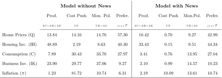
Which unanticipated shocks loose importance once we introduce news shocks? To address this question, we compare the role of the unanticipated shocks in the estimated model with news shocks (ux;t = "0x;t +"x;t4 4 +"8x;t 8) against the estimated model without news shocks (ux;t =

"0_x;t). See Table 7. In the model without news shocks, cost-push shocks are as important as productivity and monetary policy shocks in accounting for the observed variability in house prices and business investment. Cost-push shocks are also a main source of ‡uctuations in consumption. The introduction of news shocks as a source of ‡uctuations signi…cantly reduces the importance of unanticipated cost-push shocks and gives a predominant role to the anticipated component of this shock. As for residential investment, consumption and business investment we also …nd a less sizable role for productivity and monetary factors. The importance of the unanticipated component of all shocks is signi…cantly reduced for house prices.

2 4_{Lambertini, Mendicino and Punzi (2010) document that, over the last three decades, housing prices boom-bust}

cycles in the U. S. have been characterized on average by co-movement in GDP, consumption, business investment, hours worked, real wages and housing investment.

2 5_{See, among others, Iacoviello (2005), Iacoviello and Neri (2010), Christensen, Corrigan, Mendicino and Nishiyama}

6

Boom-Bust Cycles in House Prices

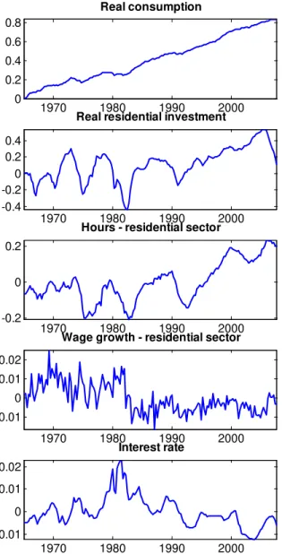
In this section, we quantify the contribution of di¤erent shocks to house price growth over boom-bust episodes. To identify the main cycles in real house prices, we use the Bry-Boschan algorithm with a one-year minimum criterion to de…ne a cycle phase. The peaks and troughs of the four cycles identi…ed with this method coincide with local maxima and minima of the real house price series. See Figure 6. We report the results for the two main booms that peak in 1979Q4 and 2005Q4, respectively. Real residential investment displays co-movement with house prices during the …rst two decades of the sample. The peaks in residential investment anticipate the peaks in house prices only by one quarter. In contrast, during the last two decades, the cycles of residential investment and house prices are unsynchronized. House prices generally increase since the mid-1990’s to 2005Q3. In contrast, residential investment displays a di¤erent pattern and more closely follow the U.S. economic cycle. Leading the NBER business activity peak by a few quarters, the series displays a peak in 2000Q3, whereas the decline in housing investment ends in 2003Q1, a few quarters after the through of activity. Thus, we also consider an alternative cycle for residential investment peaking in 2000Q3, as identi…ed by the Bry-Boschan algorithm.

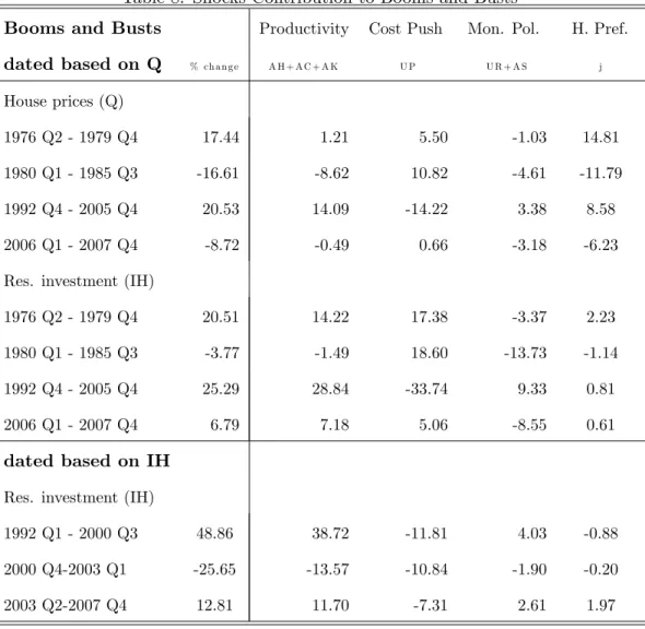
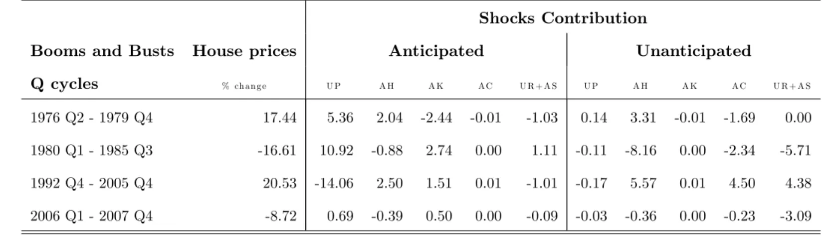
Table 8 reports the contribution of the estimated shocks to house prices and residential in-vestment growth during each boom- and bust-phase. Adding up the contribution of news and unanticipated shocks we …nd that: (i) cost-push shocks display a sizable contribution to the run up in house prices and residential investment of the late 1970’s; (ii) monetary and productivity factors are found to be important for the subsequent bust; (iii) productivity accounts for more than half of the increase in house prices and residential investment during the most recent period; (iv) monetary factors signi…cantly contribute to the early bust-phase of the more recent cycle in house prices; (v) housing preference shocks signi…cantly contribute to changes in house prices, whereas the contribution of these shocks to changes in residential investment is not sizable.

Is there any role for news shocks during housing market booms and busts? Regarding the relative importance of the anticipated and unanticipated component of shocks for changes in house prices, news shocks contribute to the boom-phases, whereas the busts are almost entirely the result of unanticipated monetary policy and productivity shocks. News shocks also sizably contributed to changes in residential investment. See Tables 9 and 10.

market dynamics during the entire 1970’s.26 _{News on cost push shocks is arguably related to}

ex-pectations of oil price shocks. In fact, in 1973 and 1979 most of the industrialized nations, including the U.S. experienced two major oil crises mainly on account of disruptions to energy supply. It is common in DSGE models to explain the in‡ationary pressures generated by the dramatic increase in oil prices through cost push shocks.27 Once we allow for news on the cost push shock, we …nd that expectations about future in‡ationary pressures were more important than current shocks in determining agents’ housing investment decisions during the high in‡ation period of the 1970’s. In the next section we investigate the relationships between in‡ation expectations, news shocks and housing market dynamics.28

Supporting the idea of a productivity-driven economic expansion mainly related to expectations of a "New Economy", investment speci…c news shocks were the main contributors to residential investment growth during the second-half of the 1990’s.29 Further, investment speci…c news shocks together with expectations of downward cost pressures on in‡ation account entirely for the sub-sequent decline. Despite a more sizable role for the unanticipated component of productivity and monetary policy shocks, news about productivity shocks in the housing sector and investment spe-ci…c news shocks account together for about 20 percent of the increase in house prices over the latest boom. The contribution of news about cost-push shocks also considerably muted the run up in house prices over its entire boom phase.

Summarizing, expectation-driven cycles are mainly related to news regarding cost-push shocks, shocks to productivity in the housing sector and investment-speci…c technology shocks. In contrast, the contribution of the unanticipated component of the shocks is mainly related to monetary factors and productivity in the two sectors of production.

7

Interpreting News Shocks: the Role of Expectations

Results presented above show that news about future cost-push, housing productivity, and invest-ment speci…c shocks are important sources of housing market ‡uctuations. Given that the e¤ect of news shocks mainly works through expectations, we now investigate the importance of expectations

2 6_{As for the …rst cycle of the early 1970’s, news on in‡ation and housing productivity together account for about}

17 percent of the boom and 65 percent of the bust in house prices.

2 7_{De Graeve et al. (2009) relying on an estimated macro-…nance model argue that the 1973 in‡ation hike is}

attrib-utable to wage and price-markup shocks. Several papers have documented the role of oil shocks for macroeconomic developments in the 1970s. See, among others, the seminal work by Bruno and Sachs (1985). The impact of a change in the price of oil has also been found to have decreased over time. See Blanchard and Gali (2009) and the references therein.

2 8_{Regarding in‡ation expectations and credit and real estate dynamics see also Piazzesi and Schneider (2010).} 2 9_{See, among others, Jerman and Quadrini (2003) and Shiller (2000) for detailed account on productivity growth}

for the transmission of news shocks to house prices. The assumption of nominal debt contracts suggests a role for both in‡ation and interest rates expectations in the housing and credit decisions of households. The housing pricing equation derived from the model can be expressed as

qt=Et 1j X

j=0

(~)juc;t+j

uc;t

uh;t+j

uc;t+j

, (1)

where t;t+j = ~j u_uc;t_c;t+j is the stochastic discount factor or pricing kernel and uh;t+j

uc;t+j is the marginal

rate of substitution between housing and consumption.30 Agents choose housing and consumption goods such that the sum of the current and expected marginal rate of substitution between the two goods, discounted by ~j uc;t+j

uc;t ;is equal to the relative price of houses.

31 _{Movements in the real}

interest rate, i.e. the inverse of the pricing kernel, determine house price dynamics. Since debt contracts are in nominal terms, expected in‡ation a¤ects the debt decisions of the households and also enters the optimality condition for housing investment. Lower expected real rates, through either higher expected in‡ation rates or lower interest rates, induce households to borrow more and to increase their housing investment, therefore contributing to an increase in house prices and credit ‡ows.

We proceed in two steps. First, we quantify the contribution of news shocks to model-based expectations and test the model’s ability to match survey-based expectations. Second, we explore the linkages between agents’ expectations and house prices.

7.1 Survey- versus Model-based Expectations

Are news shocks related to agents’ expectations? Table 11 reports the variance decomposition of the model-based expectations about in‡ation and interest rates generated over the sample period.32 In‡ation expectations are mostly explained by the anticipated component of the cost-push shock and the shock to the target of the central bank. In particular, news of future in‡ationary shocks explain around 50 percent of the variability in both 1- and 4-quarter ahead in‡ation expectations, with a predominant role for news shocks over longer horizon. Interest rate expectations are also driven by news of in‡ation targeting shocks and investment speci…c shocks. The importance of the anticipated components of the investment speci…c shock is plausibly related to the GDP component

3 0_{Solving forward the lender’s f.o.c. for housing it is possible to derive the equilibrium housing price equation (1),}

where the discount factor is de…ned as ~ GC(1 h).

3 1_{The house prices equation could alternatively be derived from the Borrowers’ housing demand. In this latter case}

it would involve the lagrange multiplier of the borrowing constraint. In equilibrium both speci…cation hold.

3 2_{The type of heterogeneity featured by the model does not imply heterogeneity in agents’ expectations. Both}

of the interest-rate rule. In fact, investment speci…c news shocks are among the driving forces of investment which itself represents a signi…cant share of GDP.33

As an alternative validation of the model, we assess the plausibility of the model implied ex-pectations by relating them to survey estimates of expected in‡ation and interest rates, which are not part of the information set of the model.34 We measure observed in‡ation expectations us-ing the 1- and 4-quarter ahead expected GDP de‡ator quarterly change estimated by the Federal Reserve Bank of Philadelphia Survey of Professional Forecasters (SPF). Alternatively, we also use the expected change in prices from the University of Michigan Survey of Consumers.35 _Interest

rate expectations are measured by the 1- and 4-quarter ahead expectations for the three-month Treasury bill rate provided by the SPF. We …nd that both in‡ation and interest rates expectations generated by the model are in line with the survey-based expectations. See Figure 7.

Next, we evaluate the information content of news shocks for the observed expectations on the base of Granger causality tests. We focus on the news shocks that are more relevant to each type of expectations generated by the model. The results of the test show that news shocks contain statist-ically signi…cant information for all measures of observed in‡ation and interest rate expectations. See Tables 12 and 13.36 _{Thus, news shocks are found to be important in explaining model-generated}

expectations about in‡ation and interest rates. Further, they also contain signi…cant information for survey-based expectations.

7.2 Expectations and House Prices

Next, we explore the relationship between expectations and house prices. The link documented above between news shocks and agents’ expectations suggests an important role for both in‡a-tion and interest rate expectain‡a-tions in house prices ‡uctuain‡a-tions. Table 14 reports the correlain‡a-tions between house prices and expectations over the observed boom and bust episodes. Survey based in‡ation expectations are strongly positively correlated with house prices during the boom-bust cycle of the late 1970’s. In contrast, the correlation becomes weaker during the more recent cycle. Observed interest rate expectations are negatively correlated with house prices during the recent boom and positively correlated during the bust-phase. See also Figure 8. One plausible reason for the weaker co-movement of in‡ation expectations and house prices during the more recent boom,

3 3_{Expectations on in‡ation and interest rates are not among the observables used in the estimation.}

3 4_{Previous papers that explore the ability of DSGE models to …t the dynamics of in‡ation expectations focus on}

alternative assumptions regarding agents’ information on the target of the central bank. See, i.e., Schorfheide (2005) and Del Negro and Eusepi (2010).

3 5_{In the Michigan survey, the question asked is "By what percent do you expect prices to go up, on the average,}

during the next 12 months?". We use the mean of the responses to this question.

3 6_{The number of lags included in the tests was chosen based on the Akaike information criteria. The results are}

could be related to the ability of the monetary authority to stabilize both in‡ation and in‡ation expectations since the mid-1980’s. This could also explain the countercyclical behavior of interest rate expectations during the latest house price boom. In fact, under more stable in‡ation expecta-tions, expected lower future real rates would be mainly related to expectations of a lower nominal interest rate.37

As for the model-based expectations, in‡ation expectations are positively correlated with house prices during the boom-bust episodes, whereas the relationship between interest rate expectations and house prices varies through time and became negative during the most recent period of run up in house prices. See Table 14. By visual inspection, we can see that the expected interest rate declined during the early phase of the more recent boom (2000Q3-2004Q1) and the trough in interest rate expectations anticipate the peak in house prices.

Interest rate expectations in the model are mainly driven by the systematic component of the policy rule. In fact, interest rate expectations seem to be strongly linked to expectations regarding both in‡ation and GDP growth as opposed to news about monetary policy shocks. The negative correlation between house prices and interest rate expectations during the more recent booms is explained by a decline in model-based expectations regarding GDP growth. In fact, during the early phase of the more recent house prices boom that coincided with the 2001 recession period, interest rate expectations decline given a deterioration of GDP growth expectations. See Figure 9. Summarizing, the model performs reasonably well in capturing the relationship between ex-pectations and house prices. In particular, it is able to match the co-movement between house prices and in‡ation expectations during the earlier cycles in housing prices and the counter-cyclical behavior of interest rate expectations during the more recent boom.

8

Conclusions

This paper quanti…es the role of expectations-driven cycles for housing market ‡uctuations in the United States. Due to their ability to generate pro-cyclical and hump-shaped dynamics, news shocks emerge as relevant sources of macroeconomic ‡uctuations and explain a sizable fraction of

3 7_{Piazzesi and Schneider (2010) input survey-based expectations into an endowment model economy with nominal}

variation in house prices and housing investment and more than half of the variation in consumption and business investment. Housing productivity, investment-speci…c and cost-push news shocks, are among the main sources of business cycle ‡uctuations.

References

[1] Adam, K., Kuang, P. and A. Marcet, 2011. House Price Booms and the Current Account. NBER Working Paper No. 17224, July.

[2] Adolfson, M., S. Laseen, J. Linde, and M. Villani, 2007. Bayesian Estimation of an Open Economy DSGE model with Incomplete Pass-Through. Journal of International Economics

72(2): 481-511.

[3] An, S. and F. Schorfheide, 2007. Bayesian Analysis of DSGE Models. Econometric Reviews, 26(2): 113-172.

[4] Aoki, K., Proudman, J. and G. Vlieghe, 2004. House prices, consumption, and monetary policy: a …nancial accelerator approach. Journal of Financial Intermediation, 13(4): 414-435.

[5] Badarinza, C. and E. Margaritov, 2011. News and Policy Foresight in a Macro-Finance Model of the US. ECB Working Paper No. 1313.

[6] Barsky, R. B. and E. R. Sims, 2009. News Shocks, mimeo.

[7] Beaudry, P. and F. Portier, 2004. An Exploration into Pigou’s Theory of Cycles. Journal of Monetary Economics, 51: 1183-1216.

[8] Beaudry, P. and F. Portier, 2006. Stock Prices, News, and Economic Fluctuations. American Economic Review, 96(4): 1293-1307.

[9] Beaudry, P. and F. Portier, 2007. When can Changes in Expectations Cause Business Cycle Fluctuations in Neo-classical Settings?.Journal of Economic Theory, 135(1): 458-477.

[10] Blanchard, O. and J. Gali, 2009. The Macroeconomic E¤ects of Oil Price Shocks: Why are the 2000s so di¤erent from the 1970s?. in J. Gali and M. Gertler (eds.), International Dimensions of Monetary Policy, University of Chicago Press (Chicago, IL): 373-428.

[11] Bruno, M. and J. Sachs, 1985. Economics of Worldwide Stag‡ation. Harvard University Press: Cambridge Massachusetts.

[12] Burnside, C. M. Eichenbaum and S. Rebelo, 2011. Understanding Booms and Busts in Housing Markets. NBER Working Paper No.16734, January.

[14] Case, K. E. and R. J. Shiller, 2003. Is there a bubble in the housing market?.Brookings Papers on Economic Activity, 2: 299-361.

[15] Campbell, J. R. and Z. Hercowitz, 2004. The Role of Collateralized Household Debt in Mac-roeconomic Stabilization. NBER Working Paper No. 11330.

[16] Christensen, I., P. Corrigan, C. Mendicino and S. Nishiyama, 2009. Consumption, Housing Collateral, and the Canadian Business Cycle, Bank of Canada Working Paper 2009-26.

[17] Christiano, L., C. Ilut, R. Motto, and M. Rostagno. 2008. Monetary Policy and Stock Market Boom-Bust Cycles. ECB Working Paper Series 955.

[18] Davis, M. and J. Heathcote, 2005. Housing and the Business Cycle. International Economic Review, 46 (3): 751-784.

[19] Del Negro, M. and S. Eusepi, 2010. Fitting Observed In‡ation Expectations. Federal Reserve Bank of New York Sta¤ Reports 476, November.

[20] De Graeve, F., Emiris, M. and R. Wouters, 2009. A Strucural Decomposition of the US Yield Curve.Journal of Monetary Economics, 56, 545.

[21] Fernández-Villaverde, J., 2010. The Econometrics of DSGE Models. SERIES: Journal of the Spanish Economic Association, 1: 3-49

[22] Finocchiaro, D. and V. Queijo von Heideken, 2009. Do Central Banks React to House Prices?. Sveriges Riksbank, Working Papers Series No. 217.

[23] Floden, M., 2007. Vintage Capital and Expectations Driven Business Cycles. CEPR Discussion Paper 6113.

[24] Fujiwara, I., Y. Hirose, and M. Shintani, 2001. Can News be a Major Source of Aggregate Fluctuations? A Bayesian DSGE Approach. Journal of Money, Credit and Banking, 43(1): 1-29.

[25] Iacoviello, M., 2005. House Prices, Borrowing Constraints, and Monetary Policy in the Business Cycle.American Economic Review,95(3): 739-64.

[26] Iacoviello, M. and R. Minetti, 2006. International Business Cycles with Domestic and Foreign Lenders.Journal of Monetary Economics, 53(8): 2267-2282.

[28] In’tVeld, J., Raciborski, Ratto and Roeger, 2011. The recent boom–bust cycle: The relative contribution of capital ‡ows, credit supply and asset bubbles. European Economic Review, 55(2011): 386–406.

[29] Iskrev, N., 2010a. Local Identi…cation in DSGE Models. Journal of Monetary Economics, 57(2): 189-202.

[30] Iskrev, N., 2010b. Evaluating the strength of identi…cation in DSGE models. An a priori approach, Working Papers 2010j32, Banco de Portugal.

[31] Je¤reys, H., 1961.Theory of Probability,Oxford University Press: Oxford, U.K.

[32] Jermann, U. and V. Quadrini, 2007. Stock Market Boom and the Productivity Gains of the 1990s.Journal of Monetary Economics, 54(2): 189-202.

[33] Khan H. and J, Tsoukalas, 2010. The Quantitative Importance of News Shocks in Estimated DSGE Models, mimeo.

[34] Kass, R. E. and A. E. Raftery, 1995. Bayes Factors.Journal of the American Statistical Asso-ciation, 90(430): 773-795.

[35] Kiyotaki, N. and J. Moore, 1997. Credit Cycles.Journal of Political Economy,105(2): 211-48.

[36] Kiyotaki, N., Michaelides, A. and Nikolov, K., 2010. Winners and Losers in Housing Markets. forthcomingJournal of Money, Credit and Banking.

[37] Kurmann, A. and C. Otrok, 2010. News Shocks and the Slope of the Terms Strucure of Interest Rates, mimeo.

[38] Liu, Z., Wag, P. and T. Zha, 2011. Land-Price Dynamics and Macroeconomic Fluctuations, NBER wp 17045.

[39] Lambertini, L. C. Mendicino and M. T. Punzi, 2010. Expectations-driven cycles in the housing market. Banco de Portugal Working Paper 4/2010, May.

[40] Milani, F. and J. Treadwell, 2009. The e¤ects of monetary policy "news" and "surprises", mimeo.

[41] Nofsinger, J.R. 2011. Household Behavior and Boom/Bust Cycles, forthcoming Journal of Financial Stability.

[43] Piazzesi, M. and M. Schneider, 2010. In‡ation and the Price of Real Assets, mimeo.

[44] Schorfheide, F., 2005. Learning and monetary policy shifts. Review of Economic Dynamics,

8(2): 392–419.

[45] Schmitt-Grohe, S. and M. Uribe, 2012. What’s News in Business Cycles, mimeo, forthcoming

Econometrica.

[46] Shiller, R. J., 2000. Irrational Exuberance. Princeton University Press, Princeton, New Jersey.

[47] Sterk, V., 2010. Credit frictions and the comovement between durable and non-durable con-sumption.Journal of Monetary Economics, 57(2): 217-225.

Appendix A

A

Data

A.1 Observables

In the following we describe in detail the data used in the estimation:

Real consumption: Real Personal Consumption Expenditure (seasonally adjusted, billions of chained 2005 dollars), divided by the Civilian Noninstitutional Population. Log-transformed and normalized to zero in 1965:1.

Business Fixed Investment: Real Private Nonresidential Fixed Investment (seasonally adjus-ted, billions of chained 2005 dollars), divided by the Civilian Noninstitutional Population. Log-transformed and normalized to zero in 1965:1.

Residential Investment: Real Private Residential Fixed Investment (seasonally adjusted, bil-lions of chained 2005 dollars), divided by the Civilian Noninstitutional Population. Log-transformed and normalized to zero in 1965:1.

Hours Worked in Consumption Sector: Total Nonfarm Payrolls less all employees in the construction sector times Average Weekly Hours of Production Workers divided the Civilian Noninstitutional Population. Log-transformed and normalized to zero in 1965:1.

Hours Worked in Housing Sector: All Employees in the Construction Sector, times Average Weekly Hours of Construction Workers divided by the Civilian Noninstitutional Population. Log-transformed and normalized to zero in 1965:1.

Growth in Nominal Wage in Consumption-good Sector: Average Hourly Earnings of Produc-tion/ Nonsupervisory Workers on Private Nonfarm Payrolls, Total Private. Demeaned. Growth in Nominal Wage in Housing Sector: Average Hourly Earnings of Production/ Non-supervisory Workers in the Construction Industry. Demeaned.

Real House Prices: Census Bureau House Price Index (new one-family houses sold includ-ing value of lot) de‡ated with the implicit price de‡ator for the nonfarm business sector. Demeaned.

In‡ation: quarter-on-quarter log di¤erences in the implicit price de‡ator for output in the nonfarm business sector. Demeaned.

Nominal Short-term Interest Rate: 3-month Treasury Bill Rate (Secondary Market Rate), expressed in quarterly units. Demeaned.

1970 1980 1990 2000 0

0.2 0.4 0.6 0.8

Real consumption

1970 1980 1990 2000

0 0.5 1

Real non-residential investment

1970 1980 1990 2000

-0.4 -0.2 0 0.2 0.4

Real residential investment

1970 1980 1990 2000

-0.05 0 0.05

Hours - consumption sector

1970 1980 1990 2000

-0.2 0 0.2

Hours - residential sector

1970 1980 1990 2000

0 10 20x 10

-3 _{Wage growth - consumption sector}

1970 1980 1990 2000

-0.01 0 0.01 0.02

Wage growth - residential sector

1970 1980 1990 2000

0 0.2 0.4 0.6

Real house prices

1970 1980 1990 2000

-0.01 0 0.01 0.02

Interest rate

1970 1980 1990 2000

-0.01 0 0.01 0.02

Inflation

A.2 Expectations

The survey-based expectations data analysed in the paper are:

In‡ation expectations: 1- and 4-quarter ahead expected GDP de‡ator quarterly change es-timated by the Federal Reserve Bank of Philadelphia Survey of Professional Forecasters or, alternatively, the expected change in prices from the University of Michigan Survey of Con-sumers.38 Demeaned.

Interest rate expectations: 1- and 4-quarter ahead expectations for the three-month Treas-ury bill rate provided by the Federal Reserve Bank of Philadelphia Survey of Professional Forecasters. Demeaned.

These data are ploted in Figure A.2.

1970 1980 1990 2000

-0.02 0 0.02 0.04 0.06

Inflation expectations 1 quarter ahead

SPF

1970 1980 1990 2000

-0.02 0 0.02 0.04 0.06

Inflation expectations 4 quarters ahead

SPF Michigan

1980 1985 1990 1995 2000 2005

-0.01 -0.005 0 0.005 0.01 0.015 0.02

Interest rate expectations 1 quarter ahead

SPF

1980 1985 1990 1995 2000 2005

-0.01 -0.005 0 0.005 0.01 0.015

Interest rate expectations 4 quarters ahead

SPF

Figure A.2: Survey based expectations

3 8_{In the Michigan survey, the question asked is "By what percent do you expect prices to go up, on the average,}

Table 1: Calibrated parameters

Technology Preferences

c 0.35 0.9925

h 0.10

0

0.97

l 0.10 0.66

b 0.10

0

0.97

0.79 j 0.12

h 0.01 0.52

kc 0.025

0

0.51

kh 0.03

X 1.15 Other

Xwc 1.15 m 0.85

Xwh 1.15 s 0.975

AC 0.0032

AH 0.0008

Table 2: Estimation results

Prior Posterior

Parameter Type Mean Stdev Mean 5% 95%

Habits " B 0.50 0.075 0.3263 0.2469 0.4003

"0 B 0.50 0.075 0.6018 0.5009 0.6991

Investment adjustment costs _k;c G 10 10.01 14.9672 11.4618 18.3434

k;h G 10 10.46 10.7674 6.6969 14.9466

Calvo prob. - prices B 0.667 0.05 0.8997 0.8817 0.9181

Calvo prob. - wages cons. sector w;c B 0.667 0.05 0.8580 0.8170 0.8979

Calvo prob. - wages hous. sector w;h B 0.667 0.05 0.9020 0.8829 0.9215

Indexation - prices B 0.50 0.20 0.0446 0.0058 0.0824

Indexation - wages cons. sector w;c B 0.50 0.20 0.0535 0.0056 0.0982

Indexation - wages hous. sector w;h B 0.50 0.20 0.4844 0.2442 0.7238

Cap. utilization adjustment costs B 0.50 0.20 0.6840 0.5111 0.8622

Taylor rule - Smoothing rR B 0.75 0.10 0.6552 0.5946 0.7150

Taylor rule - In‡ation response r N 1.50 0.10 1.5654 1.4664 1.6624

Taylor rule - Output growth response rY N 0.00 0.10 0.8025 0.7066 0.9018

Autoregressive parameters

Prod. consumption sector _AC B 0.80 0.10 0.9531 0.9289 0.9772

Prod. housing sector AH B 0.80 0.10 0.9970 0.9943 0.9997

Prod. capital sector AK B 0.80 0.10 0.9756 0.9593 0.9925

Preferences - housing j B 0.80 0.10 0.9454 0.9230 0.9672

Preferences - labor B 0.80 0.10 0.9458 0.9213 0.9707

Preferences - intertemporal _z B 0.80 0.10 0.8061 0.6121 0.9600

Table 3: Estimation results (cont.)

Prior Posterior

Parameter Type Mean Stdev Mean 5% 95%

Stand. deviation - unant.shocks

Prod. consumption sector AC IG 0.001 0.01 0.0096 0.0086 0.0106

Prod. housing sector AH IG 0.001 0.01 0.0187 0.0162 0.0211

Prod. capital sector AK IG 0.001 0.01 0.0015 0.0002 0.0036

Preferences - housing j IG 0.001 0.01 0.0606 0.0431 0.0793

Preferences - labor IG 0.001 0.01 0.0589 0.0339 0.0826

Preferences - intertemporal z IG 0.001 0.01 0.0107 0.0074 0.0138

Cost push p IG 0.001 0.01 0.0016 0.0010 0.0022

Monetary policy R IG 0.001 0.01 0.0031 0.0024 0.0036

In‡ation objective s IG 0.001 0.01 0.0239 10 2 0.0178 10 2 0.0299 10 2

Stand. deviation - ant. shocks 4-q

Prod. consumption sector AC4 IG 0.0035 0.02 0.0005 0.0002 0.0010

Prod. housing sector AH4 IG 0.0035 0.02 0.0007 0.0002 0.0016

Prod. capital sector AK4 IG 0.0035 0.02 0.0006 0.0002 0.0010

Cost push p4 IG 0.0035 0.02 0.0004 0.0002 0.0008

Monetary policy R4 IG 0.0035 0.02 0.0004 0.0002 0.0006

In‡ation objective*100 s4 IG 0.0035 0.02 0.0250 10 2 0.0156 10 2 0.0344 10 2

Stand. deviation - ant. shocks: 8-q

Prod. consumption sector AC8 IG 0.0035 0.02 0.0007 0.0002 0.0014

Prod. housing sector AH8 IG 0.0035 0.02 0.0040 0.0002 0.0103

Prod. capital sector AK8 IG 0.0035 0.02 0.0094 0.0069 0.0120

Cost push p8 IG 0.0035 0.02 0.0026 0.0019 0.0034

Monetary policy R8 IG 0.0035 0.02 0.0004 0.0002 0.0007

In‡ation objective*100 s8 IG 0.0035 0.02 0.0323 10 2 0.0174 10 2 0.0474 10 2

Stand. deviation - meas.errors

Hours worked - housing n;h IG 0.001 0.01 0.1445 0.1306 0.1587

Wages - housing w;h IG 0.001 0.01 0.0081 0.0071 0.0091

Table 4: Model Comparison

No news News 4 News 4&8 Benchmark (1965-2007)

Log Marginal Data Density 4809.49 4838.97 4867.60

Di¤erence - 29.48 58.11

Implied Bayes factor 1 6.4 1012 1.7 1025

I&N data (1965-2006)

Log Marginal Data Density 4693.44 4720.69 4743.11

Di¤erence - 27.25 49.67

Implied Bayes factor 1 6.8 1011 3.7 1021

Table 5: VarianceDecomposition: Anticipated vs Unanticipated Shocks Anticipated Shocks Unanticipated Shocks

Total 4 -quarter 8-quarter Total

House Prices (Q) 36.62 1.20 35.42 63.38

Housing Inv. (IH) 12.59 0.52 12.07 87.43

Consumption (C) 54.84 1.65 53.19 45.16

Business Inv. (IK) 72.11 1.77 70.34 27.89

In‡ation ( ) 63.36 10.62 52.74 36.63

Parameters set at the posterior mean; HP …ltered series.

Table 6: Variance Decomposition

Anticipated Shocks Unanticipated Shocks

Production Cost Push Mon.Pol. Product. Cost Push Mon.Pol. Preferences

A C + A H + A K U P U R + A S A C + A H + A K U P U R + A S j+ z +

House Prices (Q) 3.62 28.52 4.48 10.42 0.70 9.27 42.99

Housing Inv. (IH) 5.18 5.29 2.12 33.43 0.15 9.51 44.34

Consumption (C) 4.22 44.65 5.97 3.41 0.76 13.95 27.04

Business Inv. (IK) 23.91 44.53 3.67 2.10 0.99 14.57 10.23

In‡ation ( ) 1.33 45.19 16.84 2.19 10.09 13.61 10.74

Table 7: Variance decomposition: News vs No-News

Unanticipated Shocks

Model without News Model with News

Prod. Cost Push Mon. Pol. Prefer. Prod. Cost Push Mon.Pol. Prefer.

A C + A H + A K U P U R + A S j+ z + A C + A H + A K U P U R + A S j+ z +

House Prices (Q) 13.84 14.16 14.70 57.30 10.42 0.70 9.27 42.99

Housing Inv. (IH) 48.89 2.19 8.63 40.30 33.43 0.15 9.51 44.34

Consumption (C) 7.89 30.43 33.70 27.97 3.41 0.76 13.95 27.04

Business Inv. (IK) 23.90 29.77 37.06 9.27 2.10 0.99 14.57 10.23

In‡ation ( ) 1.23 81.72 10.74 6.31 2.19 10.09 13.61 10.74