planning through a known environment
Ana Rodrigues1
, Pedro Costa1,3, and Jos´e Lima2,3
1
Faculty of Engineering of University of Porto, Portugal
{up201400068, pedrogc}@fe.up.pt,
2
Polytechnic Institute of Bragan¸ca, Portugal
3
INESC-TEC, Centre for Robotics in Industry and Intelligent Systems, Portugal
Abstract. One of the most important tasks for a mobile robot is to navigate in an environment. The path planning is required to design the trajectory that generates useful motions from the original to the desired position. There are several methodologies to perform the path planning. In this paper, a new method of approximate cells decomposition, called K-Framed Quadtrees is present, to which the algorithm A⋆is applied to
determine trajectories between two points. To validate the new approach, we made a comparative analysis between the present method, the grid decomposition, quadtree decomposition and framed quadtree decompo-sition. Results and implementation specifications of the four methods are presented.
Keywords: Path Planning, K-Framed Quadtree, Approximate Cells De-composition
1
Introduction
Mobile robots have inspired a number of studies in complex environments, where path planning and control of robotic systems is a concern. They must be agile, efficient and fast, avoiding collisions and situations that could endanger human who are in the same environment.
Given the current location and a destination, path planning algorithms de-termine a path to reach the desired position. Initially, it is necessary to define the configuration space, which represent all possible system configurations. This consists of two zones, the space free of an obstacle, which may belong to the trajectory to be defined for the robot, and the space occupied by obstacles. Of-ten, a reduction of the configuration space is applied, reducing the robot to a single point [1]. To do this, all obstacles must be expanded, so the trajectory to be defined is free of robot obstacle collisions.
in which the robot can move very close to obstacles, or Voronoi diagram [7], which generates a Roadmap where the distance between the robot and the ob-stacles is maximized. In this technique, the generated trajectory commonly do not correspond to the smallest possible path [2], and the probabilistic roadmap consists of the random distribution of nodes along the free space. Therefore, trajectories with narrow passages are not determined, even if they exist [3]. The algorithm Bug is the simplest algorithm in terms of implementation, which is used when without knowledge of the environment. However, it does not generate optimal trajectories [4]. The use of potential fields in path planning is based on the use of electrical potentials of physics as a heuristic to find the trajectory. However, this method has important limitations such as local minimums, which block the robot, and when the robot is in front of concave obstacles, there are several possible minimum distances, which results in oscillations between the points closest to the target. The problem of local minima may be solved by forc-ing local potential extremes to lie on the boundaries of obstacles through the use of harmonic potentials [8]. The cell decomposition consists of the decomposition of the space into cells and subsequent division into occupied or free cells. ells decomposition can be effected through exact cells, where each cell has only two possible states, totally free or fully occupied, or in approximate cells, where each cell can be free, occupied or partially free. There are several techniques to imple-ment this method, decomposition, where the map is decomposed into fixed-size cells, decomposition into quadtrees, and decomposition into framed quadtrees [5]. The approximate cell decomposition is one of the most used techniques in the path planning of mobile robots [1].
In this paper, we present a new approximate cell decomposition method called K-Framed Quadtrees which generates a graph to A-star (A⋆) that is applied to determine the best trajectory. In order to validate the new decomposition, a comparative analysis is done with the most used methods of approximate cells decomposition: grid decomposition, Quadtrees decomposition and Framed Quadtrees decomposition, that also use A⋆.
2
Approximate Cells Decomposition
Initially, an expansion of the obstacle area is performed with the dimensions of the robot, to allow a free of collisions path. This allows the robot to be considered as a point in space.
2.1 Grid Decomposition
and consequently, there are more areas of the map considered to be wrongly occupied.
The size of the cells affects the performance of graph search algorithm sub-sequently applied, since the smaller the cell size, the greater the number of cells to analyze. This increases processing time, but the defined path will be closer to the optimal. The chosen cell size should be enough to maximize the speed of search algorithms, while allowing the access to most areas of the map.
In this work, the neighbor cells are determined through a search with connec-tivity 8 around the current cell, where the state of each is stored in a state vector in the positionx+y×numberOf CellsP erLine, where xand y correspond to the Cell indexes inXX andY Y.
2.2 Quadtree Decomposition (QD)
Quadtree decomposition uses cells of variable size to represent the environment. The cells are successively divided into four children cells recursively, until a cell is located in a completely occupied or completely free zone or until a threshold resolution is achieved.
Quadtree is a tree data structure in which each inner node has exactly four children nodes, and each one represents a quadrant (Northwest-NW, Northeast-NE, Southwest-SW and Southeast-SE). Each cell is represented by a structure that contains the following information:
1. Initial cell position in XX andY Y 2. Size of the cell inXX andY Y
3. State of the cell: totally occupied, totally free or to be subdivided 4. Division level to which the cell belongs
5. Pointers to the 4 children cells (NW, NE, SW and SE)
This method provides great precision in areas close to obstacles. The limit resolution determines the loss of map information, i.e. a higher limit resolution allows cells of smaller size, so it will be possible to access more zones of the map, in relation to a lower limit resolution. Cells are considered neighbor cells if they share an edge and / or a vertex. Thus, if a neighbor cell is free of obstacles, the union between them may belong to a path.
2.3 Framed Quadtree Decomposition (FQD)
Framed quadtree decomposition results of an enhancement of the previous method. This algorithm consists in the addition of higher resolution cells near the perime-ter of each quadtree region. Each resulting cell is represented by a structure that contains the following information:
1. Cell’s central point position inXX andY Y
In this algorithm, when determining the neighbors of the cells generated through QD, it is necessary to store the information on the side to which the neighbor cell belongs, that is, if the neighbor cell is located North (N), South (S), west (W), east (E), northeast (NE), northwest (NW), southeast (SE) or southwest (SW) of the current cell. Once the neighbors of a parent cell (cell generated by the QD) are determined, the neighbors of a children cell (cell generated by the FQD) are higher resolution cells belonging to the same parent cell and the children cells of the neighbor cells originated by the QD, if they are within restricted limits. These limits are listed below, wherevrepresents the neighbor cell andnrepresents the current cell:
1. Ifv is a neighbor parent cell (cell originated by QD) to N or S
– The children cells (cells originated by FQD) ofvare considered neighbor cells if their position in XX is between the parent cell’s boundaries in XX of n and if v contains in itsXX boundaries the x position of n
– The children cells ofv are considered neighbor cells if their position in Y Y is between the parent cell’s boundaries in Y Y + size of children cells (S), orY Y - size of children cells (N), and if there are no flaws on the side to which v belongs (N or S) and v does not contain in itsXX boundaries the x position of n
2. Ifv is a neighbor parent cell to W or E
– The children cells ofv are considered neighbor cells if their position in Y Y is between the parent cell’s boundaries inY Y of n and if v contains in itsY Y boundaries the y position of n
– The children cells ofv are considered neighbor cells if their position in XXis between the parent cell’s boundaries inXX+size of children cells (E), or XX-size of children cells (E), and if there are no flaws on the side to which v belongs (W or E) and v does not contain in its Y Y boundaries the y position of n
3. Ifvis a neighbor parent cell to NW, NE, SW or SE, the children cell closest to the current cell is considered neighbor, if the sides to which it belongs do not exist faults.
3
K-Framed Quadtree Decomposition
This method consists of the junction of quadtree decomposition (QD) and framed quadtree decomposition (FQD). In the K-Framed Quadtree algorithm, the QD is performed in a first phase, and subsequently cells of higher resolution are added in the vicinity of the perimeter of each cell with size above the previously established lower limit,k. This allows an adjustment between the two algorithms in which at the two extreme points it is possible to have a decomposition very similar to the QD and the FQD.
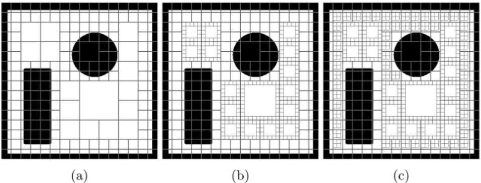
Figure 1 shows the map represented by the present algorithm. In the first instance, decomposition withk= 2.5×2.5 m results in a decomposition identical
was smaller than the size of the smallest cells. The second case is an intermediate between the QD and the FQD.
(a) (b) (c)
Fig. 1: Representation of the map through the algorithm K-Framed Quadtree. It was considered a limit for the cell size of 62×62 cm, the cells of higher resolution
have dimensions of 25×25 cm, being applied to cells with dimensions greater
than 2.5×2.5 m (Figure 1a), 1×1 m (Figure 1b) and 25×25 cm (Figure 1c).
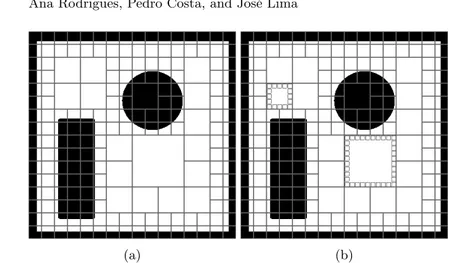
(a) (b)
Fig. 2: Representation of the map using the K-Framed Quadtrees method (Figure 2a. Changing the map representation when executing the graph search algorithm on the cells containing the start point and the destination point (Figure 2b).
When the neighbor cells originated by the QD (parent cells) are determined, is it also determined if there is a fault in the neighbor to the North (N), South (S), West (W) and East (E), that is, if any of the neighbor cells are busy. The following are some of the restrictions for a cell to be considered neighbor of the current celln.
1. If cellv is neighbor at S of celln
(a) Ifv has children cells (cells from the FQD)
i. Are considered Neighbor cells the children cells of v if cell v has within its limitsXX thexof celln
ii. If there are no faults at S of celln and ifv does not contain within the limits of XX thexof celln
A. Neighbor cells are the children cells ofv that do not exceed the limits of the parent cell ofninXX, and which do not exceed in Y Y the upper limit ofY Y of the parent cell ofnplus the size of each children cell
(b) Ifv does not have children cells i. Ifnare a parent cell
A. Cellv is considered a neighbor cell ii. Ifnare a children cell
A. vis considered to be a neighbor cell if it contains within its limits XX thexof celln
2. If cellv is neighbor at NW of celln (a) Ifv has children cells
i. If there are no failures to N and W of n or if n is a parent cell A. It is considered neighbor only the children cell ofvclosest to cell
(b) Ifv does not have children cells
i. if n is a parent cell or if there are no faults at N and W ofn, v is considered a neighbor cell
The remaining restrictions on the other sides follow the same logic.
Considering the path to be obtained, is possible to determine a coefficient that minimizes the processing time, with the application of this algorithm. The cells to be considered for the search of graphs are the cells obtained through the FQD in cells of dimensions greater thankand cells belonging to the QD if they have dimensions equal to or less than k.
4
Results
In order to evaluate the results of the different methods, processing time (t) and distance (D) associated with the path from the start point to the destination are considered. The tests were carried out on two separate maps, with dimen-sions of 10×10 m and 20.1×17.5 m. These tests were done in a simulation
environment, where all methods must give access to the same zones, that is, the loss of associated information should be the same for all methods. The graph search algorithm A-star (A⋆) is used to determine the path through the graphs that result from the previously described methods. In the tables below, the co-efficients T, l, r, and K represent the size of the cells upon grid decomposition, the lower limit of imposed parent cell size, the size of the children cells, and the minimum dimensions that the parent cells need so children cells are added in the K-Framed Quadtrees decomposition, respectively.
Algorithm T orl[cm] r[cm] k[cm] t [ms] D [m]
Grid T = 30×30 - - 40 5.5
Quadtrees l= 30×30 - - 9 6.33
Framed Quadtrees l= 30×30 30×30 - 126 5.4
K-Framed Quadtrees l= 30×30 30×30 62.5×62.5 61 5.42 Table 1: Results in the first map of A⋆ applied to the grid decomposi-tion, quadtrees decomposidecomposi-tion, framed quadtrees decomposition and k-framed quadtrees decomposition.
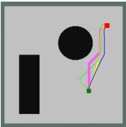
By interpreting Figure 3 and Table 1, we can verify that the trajectory with a smaller associated distance is generated by the framed quadtrees decomposition (FQD), followed by the K-Framed Quadtrees method, the grid decomposition and finally quadtrees decomposition (QD).
Regarding the processing times presented, all values are less than 200ms, however, the processing time that stands out refers to the QD being only 9ms. The remaining methods have an additional processing time cost of 31ms, 52ms, and 117ms for the grid decomposition, for the k-Framed Quadtree method, and the FQD, respectively.
Considering a small map, such as the one used for the described test, the algorithm that showed the best results was the grid decomposition, although the processing time is significantly better in quadtrees decomposition, the tra-jectory associated with this algorithm has a high additional cost in the distance, and, with the remaining algorithms, the grid decomposition algorithm presents a better processing time and a very similar trajectory, having an additional cost of about 10 cm.
The second map is a large map with narrow passages. In order to compare the methods, they must have the same loss of information and allow access to the same zones of the map. Two different paths are considered, where the starting point is equal for the two trajectories, and the destination point is different in location of the map, P1, and P2.
Algorithm T orl[cm] r[cm] k [cm] t [ms] D [m]
Grid T= 15×15 - - 1068 18.05 Quadtrees l= 15×12.5 - - 190 18.69 Framed Quadtrees l= 15×12.5 12.5×12.5 - 10184 17.80
K-Framed Quadtrees l= 15×12.5 30×30 65×62.5 411 18.41 Table 2: Results in the second map of A⋆ applied to the grid decomposi-tion, quadtrees decomposidecomposi-tion, framed quadtrees decomposition and K-framed quadtrees, to the destination pointP1.
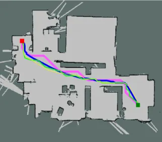
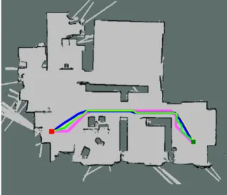
Fig. 4: Trajectories generated on the large map, by A⋆applied to the methods of grid decomposition (pink), quadtrees decomposition (green), framed quadtrees decomposition (blue) and k-framed quadtrees decomposition (yellow), to the destination pointP1.
distance of 17.80 m. The remaining trajectories generated by grid decomposition, K-framed quadtrees decomposition, and QD, have an additional cost in the path distance generated 1.4%, 3.4% and, 5%, respectively.
The QD results in the trajectory with greater distance, being this approx-imately 0.7 m higher, nevertheless the associated processing time is the most satisfactory, being only 190 ms. The path determined through the FQD is the most optimized of the paths presented, however, this method has a high pro-cessing time associated, being approximately 10 s. The grid decomposition gave a trajectory with a distance 25 cm higher than the ideal path and a processing time of 1 s. The new method resulted in a path of 18.41 m, 41 cm higher than the ideal one and a processing time of 411 ms, so there is significant improvement, in temporal terms, in relation to the grid decomposition and FQD.
Algorithm T orl[cm] r[cm] k [cm] t [ms] D [m]
Grid T= 15×15 - - 705 14.60
Quadtrees l= 15×12.5 - - 124 14.78
Framed Quadtrees l= 15×12.5 12.5×12.5 - 4776 14.46
Fig. 5: Trajectories generated on the large map, by A⋆applied to the methods of grid decomposition (pink), quadtrees decomposition (green), framed quadtrees decomposition (blue) and k-framed quadtrees (yellow), to the destination point P2.
Figure 5 and Table 3 show results of the path generated from the initial point to the target point, by the different methods implemented. The shortest path results from the FQD, which is considered the ideal route. The remaining meth-ods, in relation to the ideal path, have an additional distance cost of 0.6%, 1.0%, and 2.2%, corresponding to the K-Framed Quadtree method, the grid decom-position, and the QD, respectively. The processing times for grid decomposition and FQD are higher than those associated with the remaining algorithms. The QD has the best processing time, followed by the suggested method.
5
Conclusion and Future Work
in relation to a small decrease in the distance of the path. So, this was not considered the best method for these cases.
For the larger map, the grid decomposition obtains a longer processing time, thus becomes unsuitable for applications where a rapid response is desired. In all the tests, the QD presents very satisfactory values of processing time, however, this one originates paths further away from the considered ideal, having as char-acteristic the presence of an abrupt change of direction, in relation to the other algorithms. On the other hand, FQD presents the shortest path in most tests, but a very high processing time compared to the other methods implemented. In view of these results, a new decomposition appears, which aims, through an appropriate choice of coefficients, to obtain a compromise between the distance of the trajectory generated and the processing time. In this way, it is concluded that when using large maps with narrow passages, with an adequate choice of the coefficients associated with the k-Framed Quadtrees method, this allows better results than the others, if the objective is to obtain a good compromise between processing time and the distance of the trajectory generated. In addition, if the objective is to obtain a fast response by the algorithm, the new method is a good approach, with the proper choice of coefficients. It allows a very similar decomposition with the QD, also obtaining similar results, with an improvement of the trajectory at the beginning of the path and arrival at the destination.
As future work it would be interesting to test the algorithm in a real robot, as well as consider the orientation of the same and including dynamic obstacles.
Acknowledgment
Project ”TEC4Growth - Pervasive Intelligence, Enhancers and Proofs of Con-cept with Industrial Impact/NORTE-01-0145-FEDER-000020” is financed by the North Portugal Regional Operational. Programme (NORTE 2020), under the PORTUGAL 2020 Partnership Agreement, and through the European Re-gional Development Fund (ERDF).
This work is also financed by the ERDF – European Regional Development Fund through the Operational Programme for Competitiveness and Internation-alisation - COMPETE 2020 Programme within project POCI-01-0145-FEDER-006961, and by National Funds through the FCT – Funda¸cao para a Ciˆencia e a Tecnologia (Portuguese Foundation for Science and Technology) as part of project UID/EEA/50014/2013.
References
1. Roland Siegwart e Illah R. Nourbakhsh.: Introduction to Autonomous Mobile Robots.: Bradford Company, 2004.
3. Yunfei Zhang, N Fattahi, e Weilin Li.: Probabilistic roadmap with self-learning for path planning of a mobile robot in a dynamic and unstructured environment. IN.: Mechatronics and Automation (ICMA), 2013 IEEE International Conference on, pp. 1074–1079, 2013
4. Javier Mınguez Javier Antich, Alberto Ortiz.: A bug-inspired algorithm for efficient anytime path planning. 2008.
5. A. Yahja, A. Stentz, S. Singh, e B. L. Brumitt.: Framed-quadtree path planning for mobile robots operating in sparse environments.: In Proceedings. 1998 IEEE International Conference on Robotics and Automation
6. Han-Pang Huang and Shu-Yun Chung: Dynamic visibility graph for path planning.: In Proceedings of 2004 IEEElRSl International Conference on Intelligent Robots and Systems
7. E. J. G´omez and F. M. Santa and F. H. M. Sarmiento.: A comparative study of geometric path planning methods for a mobile robot: Potential field and Voronoi diagrams.: In 2013 II International Congress of Engineering Mechatronics and Au-tomation (CIIMA)