Pedro Miguel Botica Ferreira
Licenciado em Ciências de Engenharia BiomédicaDevelopment of a web application for processing
Neuroimaging data in the Cloud. Application to
Brain Connectivity
Dissertação para obtenção do Grau de Mestre em
Engenharia Biomédica
Orientador: Hugo Ferreira, Professor Auxiliar,
Development of a web application for processing Neuroimaging data in the Cloud. Application to Brain Connectivity
Copyright © Pedro Miguel Botica Ferreira, Faculdade de Ciências e Tecnologia, Universi-dade NOVA de Lisboa.
A Faculdade de Ciências e Tecnologia e a Universidade NOVA de Lisboa têm o direito, perpétuo e sem limites geográficos, de arquivar e publicar esta dissertação através de exemplares impressos reproduzidos em papel ou de forma digital, ou por qualquer outro meio conhecido ou que venha a ser inventado, e de a divulgar através de repositórios científicos e de admitir a sua cópia e distribuição com objetivos educacionais ou de inves-tigação, não comerciais, desde que seja dado crédito ao autor e editor.
A c k n o w l e d g e m e n t s
Firstly, I must express appreciation for my thesis advisor prof. Hugo Ferreira both for proposing an interesting and challenging thesis topic and for the help given throughout the entire work process. Secondly, my thanks to Instituto de Biofísica e Engenharia Biomédica (IBEB) for providing me with a workspace and allowing me to meet so many amazing people.
After over 5 years, I feel a great deal of gratitude not only to FCT-NOVA but also to the great minds I had the honour to meet along the way. My thanks go to prof. Mário Secca, prof. Carla Quintão Pereira and so many others which have had an impact in my academic journey and helped me see the world in new ways.
Of course none of it would have been possible without my family: my father, my mother, my brother and my grandmother. Thank you for just everything. For allowing me the possibility to take this path, for the confidence placed in me, for the uncondi-tional support. Thank you for enabling me to make these choices and supporting me all throughout. Thank you for the love you bear me and know it is returned. A special word of appreciation for my godparents could not go unsaid. Thank you for being an integral part of my life and my family, and to my godmother Paula for being a unwavering beacon of happiness.
Beyond the education I received these past years, I have been fortunate enough to meet amazing people who have been an integral part of not only my academic journey but my personal life as well. One friend in particular started this journey with me, and together we reach the finish line. José Trindade, thank you old chap. Others I met along the way, each adding their own colour to this 5 year canvas: Pedro Torcato, Hugo Santos, Filipe Valadas and many others. Thank you all for your friendship, for all the joy, the laughs and even the stressful moments we shared. A shout out goes, of course, to my friend all the way from Finland, Aleksi Sorvali. Kiitos paljon for coming to visit and for hosting me in Finland.
your help and guidance throughout this whole year, for putting up with my idiosyncrasies always with a smile and for helping me fill the lab with laughter and the whiteboard with random drawings.
A b s t r a c t
Neuropsychiatric disorders, or mental disorders, have long been known to be a major cause of burden to society and it is estimated that one in every four people worldwide will be affected by one of these conditions during their lifetime. The diagnosis of these conditions is based on a set of subjective criteria and on the experience of physicians and is therefore highly prone to error. Alcohol Use Disorder (AUD) is one such disorder with particularly devastating consequences to both individual and society, representing a total of 5.1% of the global burden of disease and injury. As image classification methods improve, reaching near-human capabilities, and research on brain physiology continues to advance and allow us to better understand brain structure and function through novel methods such as Brain Connectivity analysis, ingenious approaches to medical diagnosis can be envisioned. Furthermore, as new technologies allow the world to be more con-nected and less dependent on physical machinery, there is an interest in bringing this vision to both healthcare and biomedical research, through technologies such as Cloud computing.
This work focuses on the creation of an intuitive Cloud-based application which uses the image classification algorithm Convolutional Neural Network (CNN). The applica-tion would then be used to classify Electroencephalography data to diagnose AUD, in particular using Brain Connectivity metrics.
The created application was successfully developed according to the objectives, prov-ing to be simple to operate but effective in the use of the CNN algorithm. However, due to the environment used, it showed high processing times which hamper the training of CNN classifiers. Classification results, while not conclusive, show indication that the employed metrics and methodology may be of use in the context of neuropsychiatric dis-order diagnosis both in a research and clinical context in the future. Finally, discussion and analysis of these results were performed so as to drive forward the research into this methodology.
R e s u m o
Os distúrbios neuropsiquiátricos são das enfermidades com maior impacto mundial, estimando-se que afectem uma em cada quatro pessoas durante a sua vida. O diagnós-tico destas doenças é baseado num conjunto de critérios subjectivos e na experiência do profissional de saúde que o conduz, estando sujeito a erro humano. O alcoolismo, um destes distúrbios, é particularmente devastador, sendo o consumo de álcool responsável por 5.1% do impacto causado por todas as doenças. À medida que os métodos de classi-ficação de imagem melhoram e a investigação na área da fisiologia cerebral nos permite compreender o funcionamento do cérebro através de métodos inovadores de análise de Conectividade Cerebral, novas metodologias de diagnóstico clínico podem ser concebi-das. Além do mais, a passo com a forma como novas tecnologias interligam o mundo e reduzem a dependência em maquinaria física, surge o interesse em trazer esta visão ao cuidado médico e à investigação biomédica com tecnologias como computação emCloud. Este trabalho foca-se na criação de uma aplicação emCloudque seja intuitiva e use o
algoritmo de classificação de imagem Redes Neuronais Convolucionais. Esta aplicação foi usada para classificar dados electroencefalográficos de modo a diagnosticar alcoolismo usando métricas de Conectividade Cerebral.
A aplicação foi criada de acordo com as especificações, sendo muito intuitiva mas também eficiente no seu uso do algoritmo pretendido. No entanto, devido ao ambiente no qual foi implementado, sofre de um tempo de processamento que dificulta o treino de redes. Os resultados da classificação de dados, apesar de não serem conclusivos, mostram indícios de que as métricas e metodologia usadas poderão ser aplicadas num contexto clínico e em investigação científica. Finalmente, discussão e análise dos resultados foram realizadas de forma a desvendar potenciais direcções futuras para este trabalho.
Palavras-chave: Redes Neuronais Convolucionais, Computação em Nuvem, Alcoolismo, Aprendizagem Automática, Conectividade Cerebral
C o n t e n t s
List of Figures xv
List of Tables xvii
Acronyms xix
1 Introduction 1
1.1 Context & Motivation . . . 1
1.2 Objectives . . . 5
1.3 Thesis Overview . . . 5
2 Theoretical Concepts 7 2.1 Alcohol Use Disorder . . . 7
2.1.1 Definition & Pathophysiology . . . 7
2.1.2 Clinical Diagnosis . . . 8
2.2 Electroencephalography . . . 9
2.2.1 Introduction and Underlying Theory . . . 9
2.2.2 Analysis of Brain Connectivity . . . 11
2.2.3 Brain Connectivity in Alcohol Use Disorder . . . 13
2.3 Machine Learning . . . 14
2.3.1 Artificial Neural Networks . . . 14
2.3.2 Convolutional Neural Networks . . . 15
2.4 Cloud Computing . . . 22
2.4.1 Definition . . . 22
2.4.2 Deployment Models . . . 23
2.4.3 Cloud Service Models . . . 23
3 Materials & Methods 25 3.1 Application . . . 25
3.1.1 Theano©framework . . . 25
3.1.2 Microsoft Azure® . . . 26
3.1.3 Flask©Microframework . . . 26
3.2.1 Datasets . . . 27
3.2.2 Image Creation Methodology . . . 29
3.2.3 Network Training Configuration . . . 32
3.2.4 Cross-Validation . . . 32
4 Results & Discussion 33 4.1 Application . . . 33
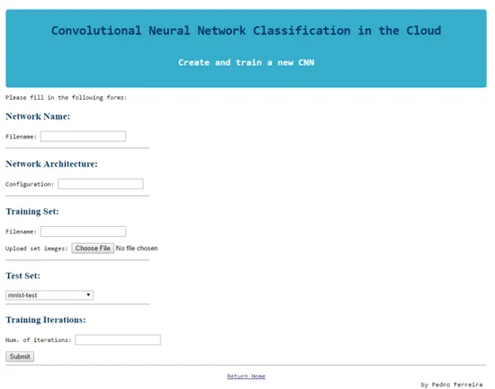
4.1.1 Interface . . . 33
4.1.2 Structure . . . 34
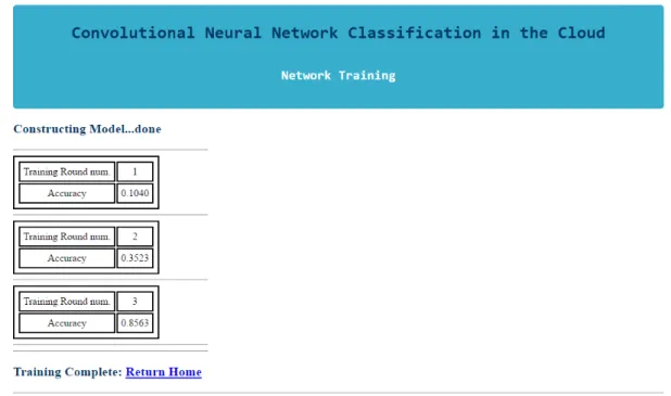
4.1.3 Network Creation and Training . . . 35
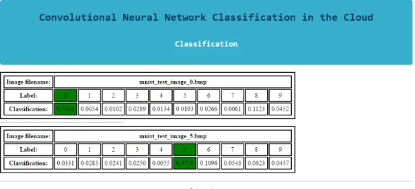
4.1.4 Data classification with an existing network . . . 38
4.1.5 Custom Network Architecture . . . 41
4.1.6 Data Labelling . . . 43
4.1.7 Use of Theano . . . 43
4.1.8 Cloud Environment . . . 43
4.1.9 Processing Time . . . 44
4.2 Classification . . . 48
4.2.1 MNIST Data . . . 48
4.2.2 Raw Data . . . 49
4.2.3 Pearson Correlation . . . 50
4.2.4 Maximum Cross-Correlation . . . 51
4.2.5 Paradigm Comparison . . . 53
4.2.6 Metric Comparison . . . 54
5 Conclusions 57 5.1 Limitations . . . 57
5.2 Future Work . . . 57
5.3 Final Thoughts . . . 58
L i s t o f F i g u r e s
2.1 Modified Combinatorial Nomenclature of the International 10/20 System . . 10
2.2 Artificial Neuron Model . . . 15
2.3 Three layered Artificial Neural Network Example . . . 16
3.1 Example of an MNIST image . . . 27
4.1 Website Main Page . . . 34
4.2 Application Structure . . . 35
4.3 Network Creation and Training Interface - Datasets Retrieval Prompt . . . . 36
4.4 Network Creation and Training Interface - Network Parameters . . . 37
4.5 Network Creation and Training - Parameter Confirmation . . . 37
4.6 Network Training Interface . . . 38
4.7 Classification Page Interface . . . 39
4.8 Network Loading Page Interface . . . 39
4.9 Classification Results Interface . . . 40
4.10 Caffe Network Upload Page Interface . . . 41
4.11 MNIST Classification Results . . . 48
4.12 Example of a Raw image . . . 49
4.13 Example of a Pearson Correlation image . . . 50
4.14 Example of a Maximum Cross-Correlation image . . . 51
L i s t o f Ta b l e s
3.1 Training and Testing Set detail . . . 29
4.1 Training Round Duration Table . . . 45
4.2 Training Round Duration Per Image Table . . . 46
4.3 Testing Round Duration Table . . . 46
4.4 Testing Round Duration Per Image Table . . . 46
4.5 Results of the Raw metric . . . 49
4.6 Results of the Pearson Correlation metric . . . 51
A c r o n y m s
ANN Artificial Neural Network. AUD Alcohol Use Disorder.
BCI Brain-Computer Interface.
CNN Convolutional Neural Network.
CPU Central Processing Unit.
CSS Cascading Style Sheets.
ECG Electrocardiography.
EEG Electroencephalography.
fMRI Functional Magnetic Resonance Imaging.
GABA Gamma-aminobutyric Acid.
GPU Graphics Processing Unit.
HTML HyperText Markup Language.
IaaS Infrastructure-as-a-Service.
IBEB Instituto de Biofísica e Engenharia Biomédica.
ML Machine Learning.
MNIST Modified National Institute of Standards and Technology.
MRI Magnetic Resonance Imaging.
NAcc Nucleus Accumbens.
NIST National Institute of Standards and Technology.
PaaS Platform-as-a-Service.
ReLU Rectified Linear Unit.
RMSProp Root Mean Square Propagation.
SaaS Software-as-a-Service.
SSD Solid-State Drive.
SUD Substance Use Disorder.
UCI University of California, Irvine.
VTA Ventral Tegmental Area.
C
h
a
p
t
e
r
1
I n t r o d u c t i o n
1.1 Context & Motivation
Neuropsychiatric disorders, or mental disorders, have an enormous impact on the world population [1–11]. Though the prevalence of these conditions varies widely between countries [12] it is estimated that, during their lifetime, one in every four people will be affected by a mental disorder [11]. According to the World Health Organization (WHO), these disorders are the most important causes of global illness-related burden, accounting for around one third of years living with disability among adults [10].
Studies have shown that mental disorders represent approximately 40% of the medical burden for young to middle-aged adults in North America [4] and that each year over one third of the European Union population suffers from mental illness, with the prevalence of disorders of the brain estimated to be much higher and representing the largest part of total disease burden in these countries [8].
Although many neuropsychiatric disorders may not present physical disabilities [13], all of these conditions greatly decrease quality of life as they progress [7], with symptoms invariantly leading to an inability to function as the disease progresses without treatment [5]. Moreover, these disorders tend to strike earlier in life and have a longer if not indefi-nite duration when compared to other classes of pathologies such as infectious diseases [5, 6]. Furthermore, the relative low importance most of these diseases are given in terms of government funding, especially in developing countries, leads to a spread in the preva-lence of these conditions, which then unavoidably increases their socio-economic burden [5].
to the amount of burden placed upon them by the disease [5]. Studies have found that caregivers often become depressed themselves, with caregiver burden for these condi-tions far surpassing that of chronic diseases [1]. This demonstrates the toll psychiatric disorders have upon society, as it has been shown that these conditions are among the most burdensome not only to patients but also to caregivers and healthcare institutions [1–8].
These conditions are also very frequently misdiagnosed, with currently employed diagnostic methods suffering from subjectiveness and a high proneness to error [7, 14– 17]. Misdiagnosis of these conditions leads to a lack of proper treatment which itself causes a worsening of symptoms [14–17].
Specifically alcoholism, formally defined as Alcohol Use Disorder (AUD), is a costly and socially devastating mental disorder [13, 18–20]. Alcohol consumption degrades indi-vidual health and heavily burdens society in terms of morbidity, mortality and disability [18]. Alcohol is, in fact, one of the most commonly consumed addictive psychoactive substances in the world [20], with its use being the cause of 5.9% of all world deaths (3.3 million per year) and a quarter of total deaths in the 20-39 year-old age group. Further-more, its use brings significant economic and social losses not only to the individual but to society as well, as 5.1% of the global burden of disease and injury is attributable to alcohol consumption [19].
While nowadays research into the pathophysiology of neuropsychiatric diseases is con-tinuously carried out, the mechanisms behind most of these conditions are still largely unknown and being unravelled at a slow pace [21]. However, research using brain func-tion analysis methods has shown that there is potential for a diagnosis applicafunc-tion which could be employed in a clinical context [21–25].
One of these methods relies on analysing the connections between different brain structures from various perspectives [26]. Specifically studying the functional links that exist in the brain, i.e. Functional Brain Connectivity Analysis, has proven to be an ef-fective method in diagnosing and gauging the severity of brain-related disorders [25– 28].
Functional Brain Connectivity is, in fact, a widely studied concept as it can give insight into how the brain’s neuron networks process information and how certain brain processes are carried out [25–28].
1 . 1 . CO N T E X T & M O T I VAT I O N
While these methods allow to obtain large amounts of data, they mostly offer results which may be complicated to subject to a direct human interpretation due to its high dimensionality. Having a good metric which encodes brain activity that can be used in diagnosis is of little value if result interpretation is difficult and may itself be subject to human error. For that reason, Machine Learning (ML) algorithms are often employed in these cases to offer not only automation but also to reduce subjectivity caused by human interpretation, and may be needed in situations where a human view may not fully encompass the full dimensionality of the data.
Besides its use in fields such as biometric recognition, gaming and marketing, ML has also seen use in medicine, such as in decoding brain states through electrocortigraphic, fMRI and scalp EEG data, with brain-computer interface technology being the driving force for this advancement [37].
ML has, in fact, been used in a wide array of biomedical applications and has proven to be a valuable tool in general healthcare [38], with notable uses including the classification of electrocardiographic and auscultatory blood pressure to diagnose heart conditions [39], identification of brain tumours from Magnetic Resonance Imaging (MRI) data [40], extraction of metabolic markers [40], patient characterization [41], abnormality detection in mammographies as aid to diagnosis [42], cancer prognosis and prediction [43] and in the study of neuropsychiatric disorders [44].
Image processing is arguably the largest application of ML that has seen great advance-ment in recent years [45]. With the developadvance-ment of modern medical imaging technologies, the need for image classification programs increased tremendously and is today one of the fastest growing fields of biomedical engineering [37].
Convolutional Neural Networks (CNNs), in particular, are one of the most advanced types of ML algorithms and have been shown to achieve near-human performance ac-curacies in image recognition tasks, and currently hold the best classification score of the Modified National Institute of Standards and Technology (MNIST) database, with an error rate of 0.21% [46]. CNNs find use in applications such as biometric identification [45], programs that learn to replicate painters’ style [47], applications that extract high-level human attributes such as gender and clothing [48], text classification [49], speech recognition [50] and facial recognition [51]. It is also worth to note that Brain-Computer Interface (BCI) is another field where the use of CNNs, in conjunction with EEG data, is undergoing research and showing promise, with accuracy results reaching 95% in stim-ulus response classification [52, 53]. Another relevant example of CNNs being used in conjunction with EEG is in biometric recognition using resting-state EEG signals [54].
[58]. Finally, the use of CNNs has shown that applying pattern recognition to the spatio-temporal dynamics of EEG with Brain Connectivity metrics can be used for epileptic seizure prediction [59].
Other particularly relevant use of ML in healthcare research are the development of an application to classify alcoholics and non-alcoholics using EEG and Neural Networks [60] and another using several different EEG analysis metrics to classify alcoholic and epileptic patients from control subjects and thus achieving accuracies of over 90% [36].
Another technology of interest that is growing in use is Cloud Computing [61–64]. This technology allows data and applications to be remotely housed and run in remote servers while providing many advantages in terms of computational resource scalability and pricing [61–63, 65, 66].
While the Cloud paradigm is not yet widely employed in healthcare mainly due to some aspects regarding security that still need resolving, it poses as a growing area of research in medicine and shows promise to change the way data is handled in healthcare [61–64].
The Cloud paradigm allows for several users to have access to the same data, allow-ing for the sharallow-ing of information among several healthcare entities such as physicians or between institutions [61–63, 65, 66]. This means Cloud computing can be used in Telemedicine both as an e-health data storage platform and as a data processing platform and can even be useful in emergency situations due to easy and fast data access [61, 62]. Patient monitoring is another application of the Cloud paradigm as physicians can access physiological data stored in the Cloud to remotely monitor test results or ongoing therapies [63], with this concept having been studied through the use of Electrocardio-graphy (ECG) data [64]. Using the same concept, Cloud systems can also be employed in patient self-management as an easy way to keep track of medical information and exam results [61, 62]. Also, using the Cloud paradigm as a way to outsource healthcare facility records and for remote data processing has shown to save money otherwise spent on hardware investment and maintenance costs. Medical imaging is another field where healthcare can benefit from the use of Cloud servers due to their remote storage and processing capabilities as medical images tend to be resource-heavy [63].
With all the information and studies presented above taken into consideration, an application could be envisioned which makes use of ML concepts, in particular capitaliz-ing on the strength of image processcapitaliz-ing algorithms such as CNN, and Brain Connectivity analysis (with EEG) as a computer-aided diagnosis tool. Moreover, developing the ap-plication in the Cloud would allow users to remotely access it and not be restricted by the hardware available to them, as well as provide a cost-effective platform flexible to continuous development.
1 . 2 . O B J E C T I V E S
due to the advanced capabilities of these algorithms, in particular CNNs.
1.2 Objectives
This thesis can be seen as having two main objectives.
The first objective is to create an intuitive Cloud-based application which allows the user to create, train and employ a specialized ML classifier.
The application is to follow a set of pre-determined core principles:
• Due to the current strength and wide use of image processing technologies, the application must follow an image processing paradigm, where the input data to be processed consists solely in images, and as such employs the CNN algorithm.
• To capitalize on modern Cloud-based technologies and the possibility of remote processing and removal of physical hardware restraints, as well as the possibility of more cost-effective deployments, the application is to be housed and run on a Cloud server.
• To allow its use in research and an easily adaptability to different contexts, it must be designed so that it is simple to learn and use.
The second objective is to employ the aforementioned application to classify neuropsy-chiatric data and thus evaluate metrics which could be used to automatically classify non-healthy subjects from control ones. A few core principles were also set in this second objective:
• Due to advantages of EEG in terms of ease of use and superior temporal resolution, it was chosen to be the type of physiological data acquisition to be used.
• Due to the fact that its diagnosis is less subjective and due to the relatively high availability of data, the disorder to be used in this work was chosen to be Alcohol Use Disorder.
1.3 Thesis Overview
The present chapter focuses on the background context of this thesis and explores how these concepts serve as motivation for the work that will subsequently be discussed. The main objectives are underlined as pertaining to the context and motivations discussed previously. This is intended to give the reader a broad scope of the different issues involved in this work and how each of them interconnect to give rise to what will be discussed in later chapters.
• Chapter 2 presents the scientific concepts which were tackled in this work. A great deal of focus was paid to CNN, as the development of the application and analysis of results is greatly related to the intricacies of the algorithm. Furthermore, the pathology of AUD was presented rather than neuropsychiatric disorders in general. This is due to the fact that AUD is the only disorder in focus throughout this work, though the research is embedded in the broader context of neuropsychiatric disorders, as discussed in the present chapter.
• Chapter 3 is intended to introduce the tools used in this work. Here, a division is made between those used in the context of application development and those used in classification efforts. In the former, the computational tools such as programming frameworks and the used Cloud environment are presented. In the latter, the used datasets are detailed as thoroughly as possible. Data processing techniques and classification parameters are also introduced.
• In Chapter 4, the developed application and classification results are presented and discussed. Again, this chapter is divided such as to segment the created application from the classification results so as to promote legibility. Both the application and the classification results are analysed from different perspectives such that different discussion topics arise and thus allowing a more complete analysis of the work and not only an adequate evaluation of results but also the discovery of new directions of research.
C
h
a
p
t
e
r
2
T h e o r e t i c a l C o n c e p t s
2.1 Alcohol Use Disorder
2.1.1 Definition & Pathophysiology
Alcohol Use Disorder (AUD), more commonly known as alcoholism, is a kind of Sub-stance Use Disorder (SUD) characterized by the excessive consumption of alcohol [13]. The main feature of these disorders is a set of behavioural, cognitive and physiological phenomena showing the persistent use of the substance in spite of the problems it causes, with substance use taking on a higher priority than other matters that once held much greater importance [13, 67].
Other important features of these disorders lie in the set of symptoms experienced when substance use is discontinued, known as withdrawal, and in the intense desire or urge for the substance that may occur at any time, also known as craving [13].
Unlike other drugs of abuse, alcohol does not interact with a specific receptor or target system in the brain but rather forms complex interactions with multiple neurotransmit-ter/neuromodulator systems [68]. As such, the full scope of chemical brain processes triggered in the presence of alcohol is not yet fully understood, though several neuro-transmitter systems are known to be linked to alcohol dependence [67, 69, 70].
It is this interaction with GABA, as well as other neurotransmitter systems and the endogenous opioid system, that is thought to stimulate the release of dopamine from cells in the Ventral Tegmental Area (VTA) to the limbic system, namely to the Nucleus Accumbens (NAcc) and prefrontal cortex. This circuitry, also known as the brain’s reward system, is associated with desire, motivation and reward-based learning and is thought to play an important role in reinforcing evolutionary-beneficial behaviours. It is therefore thought that this system plays an important role in developing addiction and is thought to cause euphoria when consuming alcohol [68].
With long term exposure to alcohol, however, the brain begins to adapt by counterbal-ancing its effects, in an attempt to restore equilibrium between excitatory and inhibitory processes. As such, inhibitory neurotransmission is decreased and excitatory neurotrans-mission is increased [71]. This state of compensated equilibrium is the mark of alcohol dependence. It is important to realize that this shift in neurotransmission distribution is only in equilibrium in the presence of alcohol. In the absence of alcohol, however, a new state of reversed imbalance arises, leading to an increase in excitatory neurotransmission and a decrease in inhibitory neurotransmission. This new unbalanced state is the basis of withdrawal and causes symptoms such as seizures, delirium and anxiety and is character-ized by an intense craving of alcohol as an attempt to restore neurotransmission balance in the brain [71].
Heavy alcohol intake may lead to problems in nearly every organ system such as the cardiovascular system (e.g. cardiomiopathy), the gastrointestinal tract (e.g. gastritis, liver cirrhosis, pancreatitis), the skeletal system (e.g. osteoporosis, osteonecrosis) [13, 72] and is known to affect most of the endochrine and neurochemical systems [18, 70]. Like other SUDs, AUD has variable effects on the central and peripheral nervous systems and causes aberrations in normal brain functions which, depending on the degree of addiction, may not disappear after detoxification [13, 73]. Such effects include cognitive deficits, severe memory impairment, and degenerative changes in the cerebellum [13].
2.1.2 Clinical Diagnosis
Diagnosis of AUD, or any SUD, is based on the pathological pattern of behaviours related to substance use [13, 67]. There are eleven criteria to diagnose SUD, which can be grouped into four categories [13]:
• impaired control
• social impairment
• risky use of the substance
2 . 2 . E L E C T R O E N C E P H A LO G R A P H Y
While analysis of urine or blood samples to measure blood alcohol concentration may serve as evidence to confirm one or more criteria, diagnosis usually relies on asking ques-tions regarding the subject’s experience with alcohol. To note that it is not required that it be the subject to answer these questions, provided the answers come from reliable sources. Besides diagnosing AUD, the number of confirmed criteria also allow a quantification of the severity of the disorder, as the more criteria are verified, the higher the severity of the disorder [13, 74].
Due to the fact that no empirical analysis is employed, this method of diagnosing AUD and inferring its severity is considered subjective and frequent discussion arises regarding its accuracy [74], especially when taking into consideration that the underlying condition is highly heterogeneous in both etiology and phenotype [67]. This is common to all neuropsychiatric disorders [13].
2.2 Electroencephalography
2.2.1 Introduction and Underlying Theory
Electroencephalography (EEG) is a technique that allows the collection of data pertaining to the brain’s electrical activity [30, 75–77].
The neurons composing the brain work by moving charges to transmit information to each other, in complex networks that encode brain function [30, 75, 76]. According to Standard Electromagnetic Theory, a moving charge generates an electric field which extends through space, decaying as distance to the charge increases. Thus, these small currents generate electric fields which extend to the scalp. However, due to the small magnitude of the currents produced by the activity of a single neuron, only the combined simultaneous activity of several neurons can be detected as an electric potential at the scalp [30, 75, 76]. As such, brain processes requiring the activity of a group of neurons can be acquired and amplified for analysis [30, 77]. This is the basis of EEG.
Using electrodes with a conductive material allows for the resulting electric field at the scalp to be read as an electric potential. This measurement can be stored and carried out over time to acquire a dataset of varying electric potential at specific scalp regions. The resulting data constitutes the EEG signal [30, 75–77].
placement of the electrodes can also be aided by special caps with markings of the elec-trode placement positions [30].
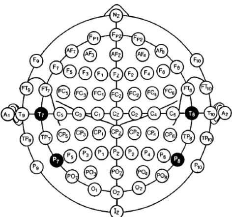
Figure 2.1: Modified Combinatorial Nomenclature of the International 10/20 System. Source: [78]
In the context of functional brain imaging, EEG can be seen to offer the following advantages [30, 33, 75–77, 79]:
• It is safe, painless and non-invasive
• The collected data can be directly correlated to brain function
• High temporal resolution (millisecond range)
• Reasonable spatial resolution (centimetre range)
• Its measurement is less restricting in terms of movement
2 . 2 . E L E C T R O E N C E P H A LO G R A P H Y
[79]. Good temporal resolution, however, proves advantageous since capturing rapid variations in neuron configurations is valuable in analysing brain function [30, 32, 33], thus leading to the choice of EEG as the physiological signal to be used in this thesis.
2.2.2 Analysis of Brain Connectivity
Mapping the human brain has been a subject of interest for neuroscientists for over a hundred years. However, there has been a recent interest in expanding this type of analysis by describing how different regions of the brain interact with one another and how these interactions depend on experimental and behavioural conditions [26].
The neuronal networks of the cerebral cortex follow two main principles of organi-zation: segregation and integration. Anatomical and functional segregation refers to the existence of specialized neurons and brain areas, organized into separate neuronal pop-ulations or brain regions. These sets of neurons selectively respond to specific stimuli and thus compose cortical areas responsible for processing specific features or sensory modalities. However, coordinated activation of dispersed cortical neurons, i.e. functional integration, is necessary for coherent perceptual and cognitive states, meaning these seg-regated neuronal populations do not work in isolation but as a part of broader processes [80]. In accordance, experiments have shown that perceptual and cognitive tasks result from activity within extensive and distributed brain networks [80].
It is the analysis of these physical and functional connections between neurons and neuronal populations that is denoted as Brain Connectivity analysis [26, 81].
When analysing brain connectivity, three different aspects can be discerned, each of which is related to different aspects of brain organization and function [80, 82–84]:
• Structural Connectivitydenotes the anatomical links between individual neurons or neuronal populations [80, 82, 83] and, more specifically, refers to white matter projections connecting cortical and subcortical regions of the brain. Analysis of this connectivity depends therefore on the scale chosen, which can range from local to inter-regional areas of the brain. Connections within the scale are thus expressed as a set of undirected connections between different elements. This kind of connectivity is thought to be quite stable on short (minute range) time scales, though this may not be true for longer time scales due to brain plasticity [83, 85].
the possible patterns of Functional Connectivity that can be generated, as anatomi-cal constraints play their part in shaping statistianatomi-cal dependence between neuronal populations [83]. Being a statistical concept, analysis of Functional Connectivity relies on statistical metrics such as correlation, covariance, spectral coherence, or phase-locking [85]. Functional brain connectivity is a widely studied concept as it can give insight into how the brain’s neuron networks process information and how certain brain processes are carried out [25–28]. Several neuropsychiatric disorders have been found to show significant changes in functional connectivity and this approach shows great promise in the study of these diseases [25–27].
• Effective Connectivityconsists in modelling directed causal effects between neural
elements to infer the influence one neuronal system has over another [83, 85]. As such, models obtained are thought to represent a possible network configuration that accounts for observed data and that therefore give insight into brain processes [83, 86]. In Effective Connectivity analysis, techniques such as network perturba-tions or time series analysis are employed [85].
Analysing functional brain connectivity is a matter of data analysis and has been applied to fMRI, EEG and MEG [26], and this analysis can be performed considering or not the temporal dynamics of the neural network [28]. Spatiotemporal functional analysis is specially interesting in this case as many psychiatric diseases show evidence of changes in functional connectivity with complex temporal dynamics [25–27].
As EEG has a high temporal resolution it allows the study of the temporal dynamics of brain activity better than other techniques [30–33] and as such has been used in the work described in this thesis. Furthermore, Pearson Correlation and Cross-Correlation are Functional Connectivity metrics [85] that were used to analyse the data.
2.2.2.1 Pearson Correlation
Pearson’s Product Moment Correlation Coefficient, or Pearson Correlation, is a frequently used method for determining the strength and direction of the linear relationship between two variables [87, 88]. It can be calculated as such [87]:
rxy=
n
P
i=1(xi−x¯)(yi−y¯)
s " n
P
i=1(xi−x¯) 2
# " n P
i=1(yi−y¯) 2
#
(2.1)
wherexandyrepresent the two variables whose relationship is being studied, ¯xand ¯
y are each variable’s average value,nis the number of data pairs between them and the resulting coefficientrxyis a value between -1 and +1.
2 . 2 . E L E C T R O E N C E P H A LO G R A P H Y
is given by the magnitude of the coefficient such that values closer to +1 or -1 will denote a stronger relationship while values closer to 0 will denote a very weak or random non-linear relationship. The direction of the relationship, on the other hand, is given by the sign of the coefficient, such that positive values imply a positive linear relationship (an increase in one variable implies an increase in the other) and negative values imply a negative linear relationship (an increase in one variable implies a decrease in the other) [87, 88].
2.2.2.2 Cross-Correlation
The Cross-Correlation function is a method for determining the strength and direction of the linear relationship between two variables as a function of the delay, or lag, between them. For two discrete time-series variablesxandy, it can be computed in the following manner [59]:
Cx,y(τ) =
1
N−τ
N−τ
P
i=1x(i)·y(i+τ), τ
>0
Cy,x(−τ), τ <0
(2.2)
whereτdenotes the lag between the signals andN is the number of samples of each signal. Interpreting the resulting value is similar to interpreting the Pearson Correlation Coefficient, except for the fact that the result only provides a correlation value for a certain lag between the signals. By analysing a Cross-Correlation spectrum of two signals, i.e. the plot of Cxy as a function of τ, it is possible to obtain information regarding the
relationship between the signals for each value of lag between them [87].
2.2.3 Brain Connectivity in Alcohol Use Disorder
Many psychiatric diseases show evidence of changes in functional connectivity with com-plex temporal dynamics [25–27].
It has been shown that alcohol does alter brain function through changes in both structural and functional connectivity [34, 89, 90]. Specifically, studies have found both a decrease in functional connectivity between the left posterior cingulate cortex and the cerebellum, and in local efficiency in the brains of subjects with AUD [34]. Also, individuals suffering from AUD show greater and more spatially expanded connectivity between the cerebellum and the postcentral gyrus, as well as restricted connectivity between the superior parietal lobe and the cerebellum [89]. The brains of alcoholics also show decoupling of synchronization between regions that are functionally synchronized in controls [34] and alcoholics show weaker within- and between-network connectivity [90] and hence evidence of abnormal connectivity [34, 89, 90].
2.3 Machine Learning
Machine Learning (ML) is a growing field and new applications are discovered on a regu-lar basis. Nowadays, ML algorithms are used in fields such as Biometrics (e.g. face, speech and handwriting recognition), search engines, fraud detection, marketing, economics and gaming [92].
Machine Learning is defined as a branch of Computer Science involved in the creation of algorithms which enable programs to learn autonomously [40, 92, 93]. It arose from the need to create algorithms to solve problems too complex to program explicitly, there-fore leading to an approach of creating programs which can generalize their procedure independently of the type of task after experiencing a learning dataset, i.e. learn from experience [40, 92].
Two fundamental ML paradigms can be identified [92, 93]:Supervisedand Unsuper-vised.
InSupervisedLearning, the program is given a data denoted as atraining set. Each member of this data set is labelled according to different classes of data. The program is then able to make inferences on a new set of data, denoted as a test set, based on the information gathered from the training set. Another set can be considered, known as the validation set, which can be seen as an additional test set, used to validate algorithm performance analysis [92, 93].
UnsupervisedLearning is similar to supervised learning with the difference that the training set is not labelled, with the program still having to segment the test set data into classes. This approach is much more complex than supervised learning but may come with benefits related to training set independence [92, 93].
2.3.1 Artificial Neural Networks
Artificial Neural Networks (ANNs) are a family of ML algorithms based on the operation of biological nervous systems, such as the human brain. ANNs are comprised of several basic computational units connected to each other in a layered network, resembling brain neurons connected through synapses. Due to this analogy, these basic units are referred to as artificial neurons and their connections as synapses [45, 94].
Due to the complexity of real neurons, the principle behind artificial ones represent an abstraction to simpler theoretical models, therefore enabling their computational representation with relative ease [45]. An artificial neuron is comprised of 3 components: the inputs, the body and the outputs [94].
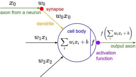
The body of the neuron represents its internal model, which can vary between neurons. The general theoretical model of the artificial neuron is given by Equation (2.3) and is illustrated in Figure 2.2 [95]:
y(x1, x2, ..., xN) =f
N X i=1
2 . 3 . M AC H I N E L E A R N I N G
wherexirepresents the value at theith neuron input out ofN such inputs,wi is the
weight associated with theith input,f represents the neuron transfer function,bis the neuron bias and finallyyis the value given at the neuron output [95].
Figure 2.2: Illustration of the artificial neuron model, with the corresponding biological equivalent components. Source: [96].
In this way, a single processing unit of the network can receive multiple inputs, each of them possessing an associated weight which determines its relative contribution to the output result, with each neuron processing its inputs in a possibly unique way by using different transfer functions. By networking several neurons it is possible to construct a complex network with strong computational abilities [45, 94, 95].
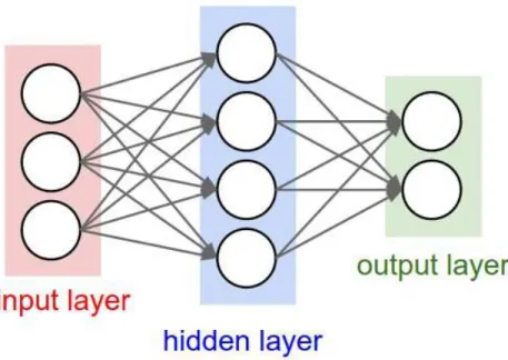
These networks are based on a 3-layered architecture in which the first layer consti-tutes the input layer, followed by a hidden layer and finally by a output layer, as shown in Figure 2.3.
While the input and output layers are fairly self-explanatory, the hidden layer is more complex. This layer receives the distributed input from the input layer and determines how stochastic changes in its parameters affect the final result, which it then transmits to the output layer. This is the basis for ML using ANNs. It is possible to have multiple hidden layers, each of which learns from the data it receives from the previous layers. This is commonly referred to as Deep Learning [51, 97].
Many types of ANNs exist, each with differences in the neuron models used and network architecture elements. This work was focused on CNNs.
2.3.2 Convolutional Neural Networks
Figure 2.3: Example of a three layered ANN with one hidden layer, three inputs and two outputs. Source: [96].
for network efficiency since it allows for a simpler and more specialized architecture and also to deal with overfitting [45].
Every data element in a set can be seen as being comprised of distinguishing features and random noise. Overfitting defines the situation where a classifier is so tuned to the training set that it learned to use the random noise present in the set to achieve a better performance. The result is a classifier with a great performance when classifying the training set, but a poor performance on unseen data. This occurs when parameter count greatly exceeds its minimum required amount. While this is unavoidable in some cases, reduction of this effect is also important in order to minimize computational resources allocated, which can be a restriction to program application, such as in cases of time or memory limitations [45, 92, 97].
Using CNNs in image processing and hence greatly reducing the number of parame-ters used in the neural net architecture leads to more time and memory efficient programs while reducing overfitting and reaping the benefits given by the robust ML approach of ANNs [97]. Furthermore, the hidden layers present in CNNs allow for deep learning where several levels of abstraction from pixels to textures can be classified, thus showing the power of this approach [48].
2.3.2.1 Convolutional Neural Network Architecture
As stated previously, CNNs were devised under the notion that inputs are comprised of images. This leads to a more specialized architecture for this kind of data than that of general ANNs [45].
2 . 3 . M AC H I N E L E A R N I N G
comprising each layer are separated into 3 different sets, each representing a dimension of the input: height, width and depth [45]. In this sense, three basic concepts are used in the CNN algorithm [97]:
• Local Receptive Fields
• Parameter Sharing
• Pooling
These concepts are realized in the special layers which compose the CNN architecture, which will be discussed in detail:
• Convolutional Layers
• Pooling Layers
• Fully-Connected Layers
Convolutional Layersare the most important layers in the CNN architecture and are in fact the core building block of these networks. They rely on the use of learnable filters, or kernels. In the Convolutional Layer, dot products are calculated between the filter and small regions of the input at different locations of the image. The filter is dragged across the image, producing a 2-dimensional activation map showing the responses of the filter at each location of the input image [45, 96].
The aforementioned principle of Parameter Sharing can be seen here, as each filter does not change depending on the location it is used in the image, and thereby reducing parameter count and ensuring that a certain feature is found in different locations in the image. Furthermore, the fact that each neuron is connected only to a limited section of the previous layer, given by each location the filter is applied at, is denoted as the neuron’s Local Receptive Field. This concept also allows for an enormous decrease in overall parameter count and model complexity [45, 96].
As these filters are learnable (i.e. their values are adjusted to improve classifier per-formance), it can be seen that certain distinguishing features of the image will produce stronger responses for each filter and non-distinguishing features will generate weaker responses. It is important to note that, while the first Convolutional layer can be easy to comprehend as it allows to determine simple changes in pixel intensity (e.g. sharp colour changes), Convolutional layers that lie further forward in the CNN architecture operate on the output of the previous layers, i.e. on these activation maps (therefore denoted as the layer’s input volume). This allows the network to distinguish more complex and widespread patterns in the input image, therefore making a CNN able to distinguish simple and complicated features in an image [45, 96].
the number of parameters required to define the network are greatly reduced, as opposed to regular ANNs, where the input volume is fully connected to the layer input. This allows for a smaller parameter count, thus reducing computational requirements and the effects of overfitting [45].
A convolutional layer is defined by a set of parameters [45, 96]:
• Filter size - this corresponds to the dimension of the filters used in this layer. Though these filters can have any 2-dimensional size, dimensions such as 3x3, 5x5 or up to 11x11 are typically used.
• Depth of the output volume - this corresponds to the number of filters that are used in the layer, each searching for different features in the input volume.
• Stride- this denotes the amount of pixel shift between 2 consecutive filter applica-tions.
• Zero-padding- this corresponds to the amount of zero-padding added to the bor-ders of the input volume.
Pooling Layersare another important layer type in CNN architecture, applying the aforementioned Pooling concept. A Pooling layer performs downsampling of its input vol-ume along the spatial dimensionality. This greatly reduces model complexity and overall parameter count, making Pooling Layers extremely important in any CNN architecture [45, 96].
The pooling layer operates in a similar manner as the convolutional layer in the sense that it also uses a filter which operates in certain locations of the image, locations which are dictated by equivalent stride and filter size hyperparameters. Hence, this layer also exhibits the concept of Local Receptive Field. However these filters are not learnable and while in the convolutional layer a dot product is calculated at each location for several filters, in the pooling layer a downsampling function is performed for a single filter. The most common downsampling function is themaxfunction, where the highest pixel value among those encompassed by the filter is selected, though averaging the pixel values is also another used approach (though much less common) [45, 96].
In terms of the size of the filter, very small filters (2x2 or 3x3) are usually preferred due to the destructive nature of the pooling layer, though larger filter sizes may be used [96].
Fully-Connected Layers are layers analogous to traditional ANNs where neurons have full connections to all activations from the previous layer. The activation volume resulting from a fully-connected layer can therefore be calculated by a simple matrix multiplication with a bias offset. As such, in order to define a Fully-Connected Layer, only the number of neurons in the layer is required [45, 96].
2 . 3 . M AC H I N E L E A R N I N G
the former has connections only to certain regions of its input volume, therefore justifying the name of the Fully-Connected Layer [96].
Rectified Linear Unit (ReLU) Layers, though sometimes not listed as CNN layers but rather as an optional operation of other layers, perform an elementwise activation function, the most common of which is thresholding at zero, as seen in Equation (2.4) [96]:
y=max(0, x) (2.4)
wherexis the input,ythe output andmaxdefines the function which outputs the largest of its input parameters.
In this work, ReLU operations are considered to be isolated layers since not doing so would lead to a degree of ambiguity regarding the point in the architecture at which the operation is performed (either before or after the associated layer). Considering it a layer eliminates this ambiguity.
Unlike the other layers presented, this layer does not present any adjustable parame-ters, but is used since it has proven to be a simple way to greatly increase training speed and effectiveness without being too demanding in terms of computational resources [96].
After all the different layers which will process data, it becomes necessary to have a manner in which the result of final layer is attributed to a class, i.e. the result is classified. As such, aScore Functionis used. Though not considered a layer, this is an indispensable part of the network architecture [96].
The network’s score function denotes the operation that computes the class scores for each prediction and is the final sequential element in a network. The 2 most commonly used are the Support Vector Machine and the Softmax functions [96]. This work will focus on the latter.
The Softmax function is a multiple class generalization of the binary Logistic Regres-sion classifier. It is used to calculate a normalized probability score that the input belongs to a certain class. Equation (2.5) describes this function [96]:
P(i) = e
xi
K
P
j=1
exj
(2.5)
2.3.2.2 Network Training
In order to train a CNN classifier, a few issues must be discussed to ensure training is effective.
In every training round, it is necessary to gauge how well the model performs so that it can adjust itself to improve performance. The algorithm used to perform this task is called aCost Function, orLoss Function. Many mathematical operations can be used to this effect, but in this work we will focus on the Categorical Cross-entropy Cost Function, which is a counterpart to the Softmax score function. It is computed using Equation (2.6), with Equation (2.7) being used to compute the total cost [96]:
Li=−log
exyi
K P j=1e xj (2.6)
L= 1
N
N
X
i=1
Li (2.7)
whereyi represents the true class of input imagei and so the argument of the loga-rithm is the Softmax function, as presented in Equation (2.5), outputting the probability score obtained for the true class of imagei. As such,Lirepresents the cost (or data loss)
associated to input image i, withL representing the average loss across allN training set images. This value is representative of network performance, where more efficient networks have a lower associatedL. The training process is guided toward the purpose of lowering this value, thus improving network performance [96].
In obtaining the model cost value, a technique must be employed to evaluate the degree of improvements that must be made to the network.Gradient Descentis a tech-nique that consists in computing the gradient of the Cost Function for each parameter throughout the training process. This way, it is possible to gauge how each parameter is affecting performance so that they can be adjusted accordingly, i.e. backpropagated [96]. Many variations of this technique exist but in this work Root Mean Square Propagation (RMSProp) will be used, which is a very effective adaptive learning rate method [98] where a moving average of the squared gradient is kept for each parameter. This process is described by Equation (2.8) and Equation (2.9) [99]:
E[g2]t=γ×E[g2]t−1+ (1−γ)×gt2 (2.8)
wt+1=wt−gt
η p
E[g2]t+ǫ
(2.9)
2 . 3 . M AC H I N E L E A R N I N G
defines the momentum term responsible for reducing oscillations in parameter optimiza-tion and is usually set to 0.9,ǫis the term responsible for decaying the moving average value in parameter update and is usually set to 1×10⁻⁶. Finally, the constantη, named
Learning Rate, is of particular interest as it dictates how strongly the gradient will affect the parameter update, hence the name. In this case, it is suggested to be set to 0.001 [99].
The next issue that must be approached is the use of Regularization techniques. These techniques focus on controlling the weight values so as to prevent the model from over-fitting the data during training. There are several Regularization techniques which find an application in CNN [96]:
• L2 regularization, or weight decay.
• L1 regularization
• Max norm constraints
• Dropout
In this work, the Dropout technique is used, as it is a very simple yet effective tech-nique.
The Dropout technique consists in only keeping a neuron active with a certain prob-abilityp, and keeping it inactive otherwise. This process of activating/deactivating neu-rons is repeated for each training round and for every neuron in the network [96].
Using Dropout, the network being trained will consist in a different configuration in every training round (though maintaining its general architecture) and the weights of each active neuron will adapt to their current configuration. While this may seem counter intuitive, it can be compared to creating several similar networks and averaging their classification results, which in itself is an effective technique to prevent a model from overfitting. The difference, however, lays in the fact that a single network is being trained, making this technique less computationally demanding [96].
The final issue is that ofWeight Initialization. Before the first training round of the network, weight values must have a starting value, which will then be adjusted as the network is trained. These values must be sensibly initialized, as they determine the point from which the network will progress through learning. If this starting point is not appropriate, then the network may never perform well [96].
A more appropriate way to initialize the weights is to assign them small random values. This method is called symmetry-breaking and allows the neurons to evolve in-dependently throughout training as unique components of a complex network, and the small magnitude of the values avoids compromising the starting state of the network. Initializing the weights in this way also avoids the need to define an initialization scheme for the bias values, as asymmetries are already avoided by the random weights, allowing the bias to also evolve independently of each other [96].
2.4 Cloud Computing
2.4.1 Definition
According to the National Institute of Standards and Technology (NIST) [100]:
Cloud Computing is a model for enabling ubiquitous, convenient, on-demand network access to a shared pool of configurable computing resources (e.g., networks, servers, storage, applications, and services) that can be rapidly provisioned and released with minimal management effort or service provider interaction.
Essentially, Cloud Computing denotes a kind of on-demand Internet-based computing where users interact with the underlying Cloud infrastructure in 5 different deployment models and 3 different service models [65, 66, 101], which will be discussed shortly.
The underlying Cloud infrastructure is composed of autonomous networked physical and abstract components. The physical components denote the hardware and the abstract ones denote the software which are the basis for the essential Cloud features presented above [65, 66, 101].
NIST also specifies 5 essential characteristics for the Cloud model [100]:
1. The user can independently access the cloud resources without the need for human interaction.
2. Cloud resources and services are available through standard network-accessing mechanisms.
3. The Cloud resources are pooled to serve multiple users simultaneously, with re-sources being dynamically assigned according to the needs of each user.
4. The Cloud capabilities are scalable and can be elastically expanded or contracted according to user and system needs.
2 . 4 . C LO U D COM P U T I N G
2.4.2 Deployment Models
NIST recognizes four different methodologies in which Access privileges to a Cloud en-vironment can be granted, and as such four different Cloud Deployment Models can be distinguished [100]:
• Public Cloud- The Cloud is accessible to the general public.
• Private Cloud - Cloud access is restricted to consumers or members of consumer organizations.
• Hybrid Cloud - Cloud infrastructure is composed of multiple distinct Cloud
in-frastructures with varying deployment models. These inin-frastructures are bound together to allow inter-Cloud operations.
• Community Cloud- Cloud access is shared between members of a community with similar concerns of whatever kind. This model stands between that of thePublic Privateclouds, as the access is not fully open but neither is it private.
2.4.3 Cloud Service Models
In the Cloud Computing model, there are three generally recognizable ways in which a Cloud provider offers their service. These differing approaches are denoted as Service Models [100]:
2.4.3.1 Software-as-a-Service (SaaS)
In this model, the user is given access to software placed on the cloud by the provider. This way, the user can remotely access capabilities which he does not own and the provider can enable that access without any product delivery. This is the more standard definition of a Cloud service and the more commonly employed. The user is given access only to the software and cannot control the underlying infrastructure, as the software should be self-sufficient in the sense that it can manage Cloud resources to ensure its correct function. SaaS is, therefore, browser interface software through a network to a Cloud [65, 66].
2.4.3.2 Platform-as-a-Service (PaaS)
2.4.3.3 Infrastructure-as-a-Service (IaaS)
C
h
a
p
t
e
r
3
M a t e r i a l s & M e t h o d s
3.1 Application
In order to develop a classifier, a ML framework which included CNN algorithms had to be chosen. The chosen framework was Theano©.
3.1.1 Theano©framework
Theano© is an open-source Python library used for the purpose of efficiently defining, optimizing and evaluating mathematical expressions involving multi-dimensional arrays. It was created in 2008 and since then has seen continuous development and multiple other frameworks have been built on top of it, including several State-of-the-Art ML models [102].
Theano was designed to function both with a Central Processing Unit (CPU) or a Graphics Processing Unit (GPU) and to facilitate the shift between them. Furthermore, the advantage of using Theano lies in its optimization techniques, as it avoids redundan-cies in computations, simplifies mathematical expressions, continuously tries to minimize both memory use and errors that arise from hardware approximations [102].
The fact that Theano is completely accessible through the Python language provides an advantage in the sense that, as long as Theano is correctly configured, one needs only to focus on developing the application front-end in Python and thus more easily separate the computational aspect of the application from the user interface. Furthermore, while Theano is widely used in the ML context, it is not solely a ML application, but rather a mathematical optimization one. This increases the advantages of using Theano in the sense that the application will be easily expandable and new features not necessarily involved in direct CNN development can be implemented [102].
To note that another ML framework was used: Caffe©, which is specialized in CNN classification [104]. One feature that was developed, as will be discussed in a later chapter, was a compatibility between this framework and the application. It was in this context that Caffe was used, and hence the application does not employ it for network training or classification of data.
3.1.2 Microsoft Azure®
Microsoft Azure® is a collection of integrated cloud computing services which can be used to create, implement and manage applications resorting to the Cloud paradigm. It provides all deployment models referenced in Section 2.4.3 and supports several pro-gramming languages, tools and frameworks [105].
Due to the inherent intricacies involved in the installation of Theano, namely the need to make changes in the file system, an IaaS approach was taken by making use of the Azure Virtual Machine functionality, where a Cloud-based virtual machine is used. Though following an IaaS approach, these environments come with a pre-installed Operating System. To create the virtual machine the user needs to select the desired computational capabilities of the environment, including pricing details.
Bearing in mind the license used, the chosen virtual machine featured a Linux Operat-ing System with a 4-core CPU, 14 gigabytes of memory and local Solid-State Drive (SSD) storage of 28 gigabytes. While virtual machines with more processing capabilities were available, including access to GPUs, the available license limited the ability to choose one such machine, and as such the most affordable virtual machine was chosen.
3.1.3 Flask©Microframework
While the classifier computations are handled by Theano, a user interface is required in order to provide a means for users to interact with the application. For this purpose, the Flask microframework was used.
Flask©is a web development microframework for Python based on Werkzeug©and
3 . 2 . C L A S S I F I CAT I O N
The fact that Jinja2 is incorporated into Flask is an especially advantageous feature. Jinja2 is a designer-friendly template engine for Python, serving as an interface between HyperText Markup Language (HTML) and Python [107]. This allows the application to interact with the HTML code which will constitute the user interface, with the underlying interface structure being handled by Flask [106, 107].
3.2 Classification
3.2.1 Datasets
Two datasets were used in this work. The first was MNIST, used only for validation of the program and network architecture, and the second was the University of California, Irvine (UCI) EEG dataset.
3.2.1.1 MNIST Database
The Modified National Institute of Standards and Technology (MNIST) database consists in a training set of sixty thousand images and a testing set of ten thousand 28×28 images
of handwritten digits (0 to 9) [108, 109]. It is an often used standard for evaluating image processing systems, especially in ML [110]. An example of an image from this database can be seen in Figure 3.1.
Figure 3.1: Example of an MNIST image, representing the number 6. Source: [109]
Images in this database consist in a black (zero-valued) background and a centred handwritten digit represented in white (maximum-valued). These images were created from original binary images which were size-normalized to fit in a 20×20 bounding box
while preserving their aspect ratio. The resulting images are, however, not binary as the anti-aliasing technique used by the normalization algorithm lead to the appearance of grey values. The centring of the images was done by translating the digits such that the pixels’ centre of mass was itself centred [109].
This database is used as a means to validate both the application algorithm and the network architecture used in this work, the latter of which is discussed in Section 3.2.3.
3.2.1.2 UCI EEG Database
The UCI Database is an open EEG database featuring time series recordings of alcoholic and healthy control subjects using 64 scalp electrodes sampled at 256 Hz during 1 second. It was obtained from the UCI Knowledge Discovery in Databases Archive athttps:// kdd.ics.uci.edu/, to which it was donated in October 1999 [111].
A total of 122 male subjects were involved in data collection. All the subjects were right-handed with normal or corrected vision. Of these 122 subjects, 77 were alcoholic and 45 were deemed healthy and as such acted as controls (and henceforth will be referred to as such) [112].
As per the alcoholic subjects, the mean age of the group was 35.83 years, with a stan-dard deviation of 5.33 and a range of 22.3 to 49.8 years. These subjects were diagnosed at the Addictive Disease Hospital in Brooklyn, New York where they were recruited and reported heavy drinking for a minimum period of 15 years. Despite this diagnosis, all subjects were detoxified and most of them had been abstaining from the consumption of alcohol for at least 28 days at the time of data acquisition. This ensures no short-term effects of alcohol use can be observed [112].
As per the control subjects, mean age was 25.81, standard deviation was 3.38 and age range was 19.4 to 38.6 years. These selected subjects reported no history of personal or family alcohol or drug abuse nor history of severe medical problems [112].
EEG data was sampled from 64 electrodes placed in accordance to the extended 10/20 International montage discussed in Section 2.2.1, with electrode impedance kept below 5 kΩ, an amplification gain of 10,000, bandpass filter between 0.02 and 50 Hz and, as
stated previously, a sample rate of 256 Hz [113].
During data acquisition, each subject was shown images from a subset of 90 pictures of objects chosen from the Snodgrass and Vanderwart picture set [114] as visual stimuli. These images represent simple objects which are easily recognizable and were presented on a white background at the centre of a computer monitor such that they were approxi-mately 5 to 10 cm in height and in width [112, 113].
Visual stimuli were presented in pairs. A first stimulus would be presented for 300 ms, followed by a fixed inter-stimulus interval of 1.6 s which then would be followed by a second stimulus. This constitutes a trial. Following the end of a trial would be another fixed interval of 3.2 s before another trial would commence. In this context, the first stimulus for each trial is referred to as S1, and the second stimulus as S2. S1 was never repeated as S1 for the same subject. However, S2 could be a repetition of S1, and in this case S2 is named S2 match. In other cases, though, S2 would not be equal to S1 but would be an image from a different semantic category, and as such be designated S2 non-match. Whether S2 would match S1 or not was randomized in each trial, with half of the trials featuring an S2 match stimulus and the other half an S2 non-match stimulus [113].
![Figure 3.1: Example of an MNIST image, representing the number 6. Source: [109]](https://thumb-eu.123doks.com/thumbv2/123dok_br/16536932.736582/47.892.342.507.648.812/figure-example-mnist-image-representing-number-source.webp)