First multi-year occultation observations of CO<sub>2</sub> in the MLT by ACE satellite: observations and analysis using the extended CMAM

(1)

ACPD

9, 11551–11587, 2009

Observations and analysis using the extended CMAM

S. R. Beagley et al.

Title Page

Abstract Introduction

Conclusions References

Tables Figures

◭ ◮

Back Close

Full Screen / Esc

Printer-friendly Version

Interactive Discussion

Atmos. Chem. Phys. Discuss., 9, 11551–11587, 2009 www.atmos-chem-phys-discuss.net/9/11551/2009/ © Author(s) 2009. This work is distributed under the Creative Commons Attribution 3.0 License.

Atmospheric Chemistry and Physics Discussions

This discussion paper is/has been under review for the journalAtmospheric Chemistry and Physics (ACP). Please refer to the corresponding final paper inACPif available.

First multi-year occultation observations

of CO

₂

in the MLT by ACE satellite:

observations and analysis using the

extended CMAM

S. R. Beagley1, C. D. Boone2, V. I. Fomichev1, J. J. Jin1, K. Semeniuk1, J. C. McConnell1, and P. F. Bernath2,3

1

Department of Earth and Space Science and Engineering, York University, Toronto, Ontario, Canada

2

Department of Chemistry, University of Waterloo, Waterloo, Ontario, Canada

3

Department of Chemistry, University of York, Heslington, York, UK

Received: 6 March 2009 – Accepted: 18 April 2009 – Published: 11 May 2009

Correspondence to: S. R. Beagley (beagley@nimbus.yorku.ca)

(2)

ACPD

9, 11551–11587, 2009

Title Page

Tables Figures

◭ ◮

Back Close

Full Screen / Esc

Abstract

This paper presents the first multi-year global set of observations of CO₂ in the mesosphere and lower thermosphere (MLT) obtained by the ACE-FTS instrument on SCISAT-I, a small Canadian satellite launched in 2003. The observations use the solar occultation technique and document the fall-o_ffin the mixing ratio of CO₂in the MLT

re-5

gion. The beginning of the fall-offof the CO₂, or “knee” occurs at about 78 km and lies higher than in the CRISTA measurements (∼70 km) but lower than in the SABER 1.06 (∼82 km) and much lower than in rocket measurements. We also present the measure-ments of CO obtained concurrently which provide important constraints for analysis.

We have compared the ACE measurements with simulations of the CO₂ and CO

dis-10

tributions in the vertically extended version of the Canadian Middle Atmosphere Model (CMAM). Applying standard chemistry we find that we cannot get agreement between

the model and ACE CO₂ observations although the CO observations are adequately

reproduced. There appears to be about a 10 km o_ffset compared to the observed ACE CO₂, with the model knee occurring too high. In analysing the disagreement, we have

15

investigated the variation of several parameters of interest, photolysis rates, formation rate for CO₂, and the impact of uncertainty in eddy di_ffusion, in order to explore pa-rameter space for this problem. Our conclusions are that there must be a loss process for CO₂, about 2–4 times faster than photolysis that will sequester the carbon in some form other than CO and we have speculated on the role of meteoritic dust as a possible

20

candidate. In addition, from this study we have highlighted a possible important role for vertical eddy diffusion in 3-D models in determining the distribution of candidate species in the mesosphere which requires further study.

1 Introduction

Carbon dioxide plays an important role in the energetics of the mesosphere and lower

25

(3)

ACPD

9, 11551–11587, 2009

Title Page

Tables Figures

◭ ◮

Back Close

Full Screen / Esc

abundance in the MLT is still uncertain. It is generally considered to be well-mixed up to at least 70 km but starts to fall offat higher altitudes due to diffusive separation and photolysis. The first CO₂ measurements in the upper atmosphere were in-situ mea-surements obtained by rocket-borne mass spectrometers (Offermann and Grossmann, 1973; Philbrick et al., 1973; Trinks and Fricke, 1978; Offermann et al., 1981). Emission

5

of the CO₂ν₃ band (asymmetric stretch mode) at 4.3µm has also been obtained from rocket measurements (e.g., Nebel et al., 1994) and from satellite by the Stratospheric and Mesospheric Sounder (SAMS) (L ´opez-Puertas and Taylor, 1989) and Improved Stratospheric and Mesospheric Sounder (ISAMS) experiments (L ´opez-Puertas et al., 1998; Zaragoza et al., 2000) up to∼120 km.

10

Global measurements of CO₂ have been obtained by the Cryogenic Infrared

Spec-trometers and Telescopes for the Atmosphere (CRISTA) experiment which was flown on two Space Shuttle missions in November 1994 and August 1997. CRISTA mea-sured CO₂4.3µm infrared emission and a non-local thermodynamic equilibrium (non-LTE) model was used to invert the radiances to CO₂number densities in the 60–130 km

15

range (Kaufmann et al., 2002). They found that the CO₂volume mixing ratio (VMR) de-viated from a well mixed state, which we will call the “knee”, around 70 km. This initial deviation is significantly lower in altitude than the result indicated by the rocket-borne mass spectrometer data mentioned above. They also found significant longitudinal and latitudinal structures in the CO₂density data.

20

More recently the Sounding of the Atmosphere using Broadband Radiometery (SABER) experiment which uses broadband radiometry to measure 4.3µm emission in the MLT region on the Thermosphere-ionosphere-Energetics and Dynamics (TIMED) satellite (e.g. Mertens et al., 2009) has provideddaytime CO₂ profiles using their ver-sion 1.06 (V1.06) retrieval method. For V1.06 retrievals their high latitude results are

25

(4)

ACPD

9, 11551–11587, 2009

Title Page

Tables Figures

◭ ◮

Back Close

Full Screen / Esc

The drawback of using emission measurements of theν₃band at 4.3µm is that this approach does not give direct information on the CO₂ abundance, but rather on the population of the vibrationally excited ν₃ level. On the other hand, the mesosphere is a region where the breakdown of local thermodynamic equilibrium (LTE) conditions starts to occur. The latter means that in order to obtain the CO₂abundance from

emis-5

sion measurements, non-LTE models must be used to interpret and invert the data. The population of the vibrationally excitedν₃level depends on the emission from this level, the absorption of near-infrared radiation emanating from the sun and from the lower atmosphere, and on collisional excitation and de-excitation by the background species, in particular by excited atomic oxygen, O(1D). There is also some evidence

10

that highly vibrationally excited hydroxyl molecules a_ffect the CO₂ asymmetric stretch mode (Kumer et al., 1978). As stated by Kaufman et al. (2002) the O(1D) excitation mechanism and the non-LTE model parameters constitute the most important uncer-tainties of retrieved CO₂. And, as noted above (Mertens et al., 2008; Remsberg et al., 2008) with broadband instruments there is the possibility of contamination from NO+

15

4.3µm emission from aurora and the ionosphere.

As mentioned above, emission instruments do not directly measure the ground state of CO₂. However, for solar occultation measurements the absorption only depends on the CO₂ density, the kinetic temperature and the pressure and not on the vibrational excitation of the CO₂ molecules. The drawback, as compared to an emission

experi-20

ment such as CRISTA is the number of profiles obtained per day. For typical low earth orbit satellites there are∼30 profiles (sunrise and sunset) per day. Solar occultation measurements of carbon dioxide have been performed on board Spacelab 1 with the grille spectrometer (Girard et al., 1988) and on Spacelab 3 by the Atmospheric Trace Molecule Spectroscopy (ATMOS) instrument (Rinsland et al., 1992) and in the

Atmo-25

spheric Laboratory for Applications and Science (ATLAS) 1, 2 and 3 missions (Kaye and Miller, 1996).

(5)

ACPD

9, 11551–11587, 2009

Title Page

Tables Figures

◭ ◮

Back Close

Full Screen / Esc

their own measurements. They employed a modified version of the US Standard at-mosphere as inputs to their retrievals (Girard et al., 1988), and (potentially significant) errors in these assumed pressure and temperature profiles would lead to errors in the retrieved CO₂VMR profile.

The ATMOS instrument had the benefit of determining pressure and temperature

5

from its own measurements, just as ACE-FTS does. However, the signal-to-noise ratio (SNR) for all but one of the occultations employed in the Spacelab 3 study (Rinsland et al., 1992) was about 74:1, much lower than that achieved by the ACE-FTS (about 350:1) in the spectral region of the strong CO₂lines. The SNR for the other occultation used in the ATMOS study was close to 200:1. There were few occultations measured

10

during the Spacelab 3 mission, yielding minimal opportunity for reducing random noise on the profiles through averaging.

2 ACE observations

The MLT CO₂ observations were obtained using the ACE-FTS, a Fourier Transform

Spectrometer, on the Canadian Atmospheric Chemistry Experiment (ACE) satellite

15

SCISAT-1 (Bernath et al., 2005). The ACE-FTS measures temperature and about thirty species involved in stratospheric ozone-related chemistry, tropospheric air quality as well as isotopologues of some of the molecules. ACE-FTS obtains solar occultations from 2.3µm to 13.3µm (750–4400 cm−1) with a high spectral resolution (0.02 cm−1). The vertical resolution is ∼3–4 km. The standard retrieval approach for temperature,

20

pressure, and VMRs are described by Boone et al. (2005).

Using software developed for the next processing version of the ACE-FTS (version 3.0), pressure/temperature (P/T) retrievals were performed for all occultations from February 2004 through August 2007, followed by CO₂VMR retrievals over the altitude range 50 to 120 km (∼1.0–2.10−5 hPa) for the same set of occultations. These CO₂

25

(6)

ACPD

9, 11551–11587, 2009

Title Page

Tables Figures

◭ ◮

Back Close

Full Screen / Esc

is perhaps excessively smoothed to be used for data analysis. However, differences between the retrieved CO₂VMR profile and the CO₂VMR profile generated during the P/T retrieval are used in the calculation of error estimates.

Both the P/T and VMR retrieval approaches employ the analysis of microwindows, small (typically∼0.4 cm−1wide) regions of the spectrum with minimal interference from

5

other molecules. The same microwindow set was used for both pressure/temperature retrievals and the subsequent VMR retrievals for CO₂. This included a number of microwindows in the range 1899–1935 cm−1(5.17–5.27µm), a set in the range 2044– 2073 cm−1 (4.82–4.89µm), and a set in the range 2293–2393 cm−1 (4.18–4.36µm). Influence of deviations from LTE is much smaller for an absorption-based instrument

10

like the ACE-FTS than for instruments measuring emission. However, to minimize pos-sible non-LTE e_ffects, all lines used in the analysis originate from the ground vibrational state. Near 2350 cm−1 (4.25µm) in particular, care was taken to avoid interferences in the microwindows from lines with excited lower state vibrations, as well as strong lines from subsidiary isotopologues of CO₂(e.g.,13CO₂). CO₂absorption is calculated

15

using the spectroscopic parameters in the HITRAN 2004 linelist (Rothman et al., 2005). The ACE-FTS CO₂observations combining both sunrise and sunset occultations are shown in Fig. 1 and are averages of the period 21 February 2004 to 30 August 2007. The coverage is not uniform and reflects that the SCISAT-1 orbit was optimized to in-vestigate the Arctic stratosphere in winter while obtaining reasonable coverage at lower

20

latitudes. The data indicate a general fall-o_ffof the CO₂VMR with height in the upper mesosphere and lower thermosphere as may be expected from the loss processes (see below). The meridional CO₂ distribution for the solstice months appears to be consistent with the large-scale circulation exhibited by the extended Canadian Middle Atmosphere Model (CMAM). As reported by McLandress et al. (2006), the meridional

25

(7)

thermo-ACPD

9, 11551–11587, 2009

Title Page

Tables Figures

◭ ◮

Back Close

Full Screen / Esc

sphere is a direct result of the resolved wave drag. This circulation pattern suggests that in the MLT subpolar summer region there should be upwelling in the lower and middle mesosphere and downwelling in the upper mesosphere. In agreement with this pattern, the January CO₂data for the austral subpolar region appear to indicate the up-welling cell up to about 85 km (∼5.10−3hPa) and downwelling cell in the region above,

5

where the descending air brings down low CO₂mixing ratios. This is also hinted at in the June/July data for boreal regions.

To estimate the error on CO₂ VMR retrieved from the ACE-FTS, three sources are considered. The first is the statistical error from the retrieval process. The second contribution comes from uncertainty in the temperature and is estimated by shifting

10

the temperature profile by a common amount of 2 K and repeating the retrieval. Note that atmospheric density (which is inversely proportional to temperature) must also be adjusted in this process to retain internal consistency. The third contribution to the error is derived from the difference between the P/T and VMR retrieval approaches. This represents a limit on the accuracy of the results due to altitude sampling and to

15

interpolation from the measurement grid to the standard 1-km grid used in the forward model calculations for the ACE-FTS. This contribution varies with the altitude spacing between measurements, and is typically larger for larger altitude spacing. The altitude spacing for ACE-FTS measurements varies over the course of a year, ranging from less than 2 km to about 6 km. The estimated errors on CO₂VMR shown in Fig. 2 use a

20

representative set of occultations with altitude spacing between 3 and 4 km. In global terms, then, the errors are generally less then 10% below 100 km.

Above the mesopause, temperature changes rapidly with altitude, and a temperature uncertainty of 2 K is possibly an underestimate. If this is true, the uncertainty at higher altitudes reported in Fig. 2 have been underestimated. In the P/T retrieval CO₂VMR is

25

(8)

ACPD

9, 11551–11587, 2009

Title Page

Tables Figures

◭ ◮

Back Close

Full Screen / Esc

3 Model

For the analysis we have used an enhanced chemistry version of the vertically ex-tended version of the CMAM model (Beagley et al., 2000, 2007; Fomichev et al., 2002; McLandress et al., 2006) with a top at 2×10−7hPa (geopotential height∼220 km but dependent on the solar cycle). The model originally contains the non-LTE

pa-5

rameterization for the 15µm CO₂ band, solar heating due to absorption by O₂ in the Schumann-Runge bands and continuum, and by O₂, N₂and O in the extreme ultravi-olet spectral region, parameterized chemical heating, molecular di_ffusion and viscosity and ion drag. The Hines (1997a, b) non-orographic GWD scheme used in the model also includes the impact of turbulence generated by the wave breaking on the

momen-10

tum budget, thermal di_ffusion and allows for di_ffusive transport of minor species; this eddy di_ffusion we call K_{Z Z}(GWD). The model also has a K_{Z Z} resulting from wind shear and a background value of K_{Z Z} for numerical control, the sum of both is generally less than 0.2 m2s−1. In addition to the numerical diffusion, tracers in the model ex-perience mixing from resolved dynamical processes such as planetary waves, gravity

15

waves and tides. This resolved diffusion is expected to be realistic. Also above∼90 km (∼0.002 hPa) vertical diffusive mixing is dominated by molecular diffusion. The model now includes comprehensive stratospheric chemistry (e.g., de Grandpre et al., 2000) with radiatively interactive O₃ and H₂O, and non-LTE treatment of the near-infrared CO₂ heating (Ogibalov and Fomichev, 2003). It also has a simplified ion chemistry

20

scheme (Beagley et al., 2007) over a vertically limited domain. The dynamical code has been modified from the earlier version (Beagley et al., 2000; Fomichev et al., 2002; McLandress et al., 2006) to allow for a 7.5 min time step without the previously used upper level enhanced horizontal di_ffusion being required. These represent the stan-dard conditions and we will explore modifications of the stanstan-dard conditions below. In

25

(9)

ACPD

9, 11551–11587, 2009

Title Page

Tables Figures

◭ ◮

Back Close

Full Screen / Esc

CO+OH→H+CO₂. Between ∼65 km and 95 km the main destruction of CO₂ is

pho-tolysis by Lyman-α with loss in the Schumann-Runge Bands (SRB) being important

below 65 km (∼0.2 hPa) and in the Schumann-Runge Continuum (SRC) being

impor-tant above 95 km (∼5.10−4hPa) (e.g., Brasseur and Solomon, 1984). Although there is some uncertainty in the CO₂ cross section at the longer wavelengths which would

5

affect photolysis below 65 km the photolysis in the main region of interest, Lyman-α, is generally well characterized. In any case we discuss the impact of the uncertain-ties below. CO is formed at all wavelengths with unit e_fficiency. Below about 45 km (∼2 hPa) CO is produced by oxidation of CH₄.

In the analysis we shall make use of this intimate connection between CO and CO₂in

10

order to provide constraints on the possibilities for agreement between measurements and model. One other point to note is that the model simulations utilized a surface boundary condition of 335 ppmv while the background CO₂for the ACE measurements is about 375 ppmv. In order to compare the vertical structures, we have scaled, in the plots, the model CO and CO₂values by this ratio to match the observations.

15

4 Results

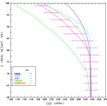
In the following we compare the ACE measurements with the CMAM results. But first we compare the ACE measurements with other experimental data including both op-tical and in-situ measurements from CRISTA, SABER and rockets. Figure 3 shows

a mean CO₂ profile based on a compilation of rocket measurements (Fomichev et

20

al., 1998), a global mean of the CRISTA measurements (Kaufmann et al., 2002), a daytime global mean (V1.06) of the SABER measurements (see above) and a global mean of the ACE measurements. Even though there are latitudinal variations in the CO₂ distribution (Fig. 1) it is clear that these di_fferences are much less than the verti-cal differences between the various measurements and the model. The CMAM global

25

(10)

ACPD

9, 11551–11587, 2009

Title Page

Tables Figures

◭ ◮

Back Close

Full Screen / Esc

above 90 km the rocket measurements fall offmore rapidly than the model results. The CRISTA measurements are the lowest with the knee commencing at∼70 km (∼0.1 hpa)

well below the ACE knee of about 78 km. However, above ∼80 km (∼0.01 hPa) the

slope of the average CRISTA and ACE results are similar. For the SABER results the

knee occurs at∼80 km, comparable to ACE measurements, but the SABER curve lies

5

∼20 ppmv higher than ACE above the knee. For the rocket measurements the knee

lies highest at∼85 km (∼5.10−3hpa). Clearly there is a discrepancy between the dif-ferent experiments with ACE and daytime SABER (V1.06) being the closest. As we noted above the derivation of CO₂ profiles from emissions measurements requires a complex non-LTE model while rocket measurements could be compromised by

sam-10

pling problems in the vicinity of the rocket skin. ACE measures the ground state of CO₂ and, hence, provides more reliable information on the CO₂abundance.

Figure 4 shows a comparison between the ACE-FTS measurements and the ex-tended CMAM, for April, for various scenarios to be discussed below. Since CMAM is a climate model we cannot compare with the same dates on which the measurements

15

were taken. However, the CMAM data averaged over the month appropriate for the ACE-FTS measurements should be representative. The ACE-FTS gives a reasonable latitudinal coverage in April and from Fig. 4 we see that the overall structure exhibited by the model for the standard scenario, A, is similar to that of the observations. How-ever, the measurements appear to have more structure with latitude. Also, the initial

20

fall-o_ff of CO₂ mixing ratio with height for the ACE measurements is clearly seen to occur at lower altitudes than for the model results in the control run, scenario A.

Prompted by the disagreement between the model and measurements we have ex-plored the conditions required to produce better agreement between the two. This was undertaken using a series of model sensitivity experiments to explore the processes

25

(11)

ACPD

9, 11551–11587, 2009

Title Page

Tables Figures

◭ ◮

Back Close

Full Screen / Esc

diffusion of chemical species associated with parameterized GWD, we introduce a sce-nario C with K_{Z Z}(GWD) neglected to explore the impact of mixing by unresolved gravity waves. Scenario D is a simulation that is a combination of B and C, i.e., both an in-creased photolysis rate for CO₂and the neglect of mixing due to K_{Z Z}(GWD). In order to explore the contribution of CO recombination to CO₂, scenario E assumes a

recom-5

bination rate for CO and OH to produce CO₂five times slower than the standard rate. For completeness, we have also investigated the impact of molecular diffusion and so for scenario F we have eliminated molecular di_ffusion for CO₂; note that molecular diffusion is retained for all the other species.

The cross-sections for each scenario for the month of April are shown in Fig. 4 and

10

the behaviour is generally what might be expected. Scenario B with the increased J

value shows that CO₂ is depleted in the MLT region compared to A. There is some

difference in the structure in the lower thermosphere where the contours are flatter for B. From scenario C it is clear that eddy di_ffusion e_ffects from GWD do have an impact, transporting CO₂ up the vertical gradient. The impact of D, i.e. a combination

15

of both B and C, is clearly excessive in terms of reducing the model CO₂ field in the MLT. For scenario E, the impact of reduced formation of CO₂ from CO is only seen below ∼0.005 hPa (∼85 km), resulting in less CO₂. Scenario F has an impact in the mesosphere resulting in a smaller CO₂ field. In the lower thermosphere the CO₂field is increased as it is maintained by the resolved wind field and is not constrained by

20

trying to achieve gravity-di_ffusive equilibrium with a concomitantly smaller scale height. Figure 5 shows a series of averaged ACE April profiles for regions where there is ample ACE data, viz.,∼30◦N, 3◦N and 80◦S respectively. Also shown are the CMAM profiles for the various scenarios listed in Table 1 which highlights more clearly the inability of the model to simulate the height at which the CO₂mixing ratio begins to fall

25

(12)

ACPD

9, 11551–11587, 2009

Title Page

Tables Figures

◭ ◮

Back Close

Full Screen / Esc

worst agreement above 100 km (∼1.10−4hPa), as might be expected, is F i.e. with no molecular diffusion. Only D, with both high J value and no K_{Z Z} from GWD, lies below the measurements.

Figure 5b shows the same comparison as 30◦N for the tropics (3◦N) for April and the results are generally the same with the increased J value giving the best agreement

5

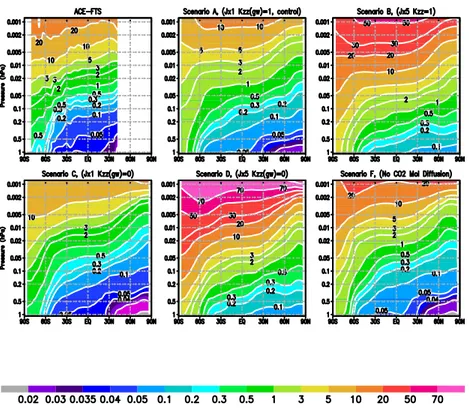
with the other scenarios generally following those seen in Fig. 5a. For austral polar regions (80◦S) the results are shown in Fig. 5c. For this case none of the scenarios provide good agreement. Even scenario B, is a poor fit and scenario D, with modified J and K_{Z Z}(GWD)₌0 is too low. Viewed as an experiment on the role of GWD this sug-gests that perhaps the K_{Z Z} generated by the GWD parameterization is strongest in the

10

polar autumnal region so that the CO₂ is diffused up the gradient to higher altitudes. This is confirmed by Fig. 6 that shows a zonally and temporally average K_{Z Z}(GWD) for the month of April. It is clearly seen that the impact of turbulence generated by unre-solved gravity wave breaking on the model mixing is most important in polar regions where K_{Z Z}(GWD) is by about an order of magnitude larger than in the tropical and

15

mid-latitude regions.

Figure 7 shows the April CO mixing ratios for ACE and for each of the scenarios for CMAM shown in Table 1. The standard scenario, A, suggests that the CMAM simulation of CO provides a reasonable representation of CO. This is not unexpected as the standard CMAM with a top at 0.001 hPa also simulates well the CO distribution

20

(Jin et al., 2005, 2008). At all latitudes the extended CMAM model CO, scenario A, is generally within 30% of the ACE CO, which, considering the rapid vertical variation of CO seems quite reasonable. However, we should bear in mind that the CO production rate calculated from the photolysis of CO₂ must be too high above 80 km since the model CO₂field is too high for the control run (A).

25

(13)

aver-ACPD

9, 11551–11587, 2009

Title Page

Tables Figures

◭ ◮

Back Close

Full Screen / Esc

aging this appears as localized descent ∼70◦S (compare Fig. 13 of Jin et al., 2008). For scenario B with increased J value we see that the CO is up to a factor of five too large at most locations and this is with a CO₂ distribution which fits the ACE obser-vations; one implication is that the removal process for CO₂ cannot simply result in production of CO. For case C with K_{Z Z}(GWD) turned o_ffthe model CO is too low by

5

∼30% at 0.002 hPa (∼90 km) but at 0.2 hPa (∼65km) the model is too high by about 30% as compared to the ACE, so that the gradient has been a_ffected by turning o_ff K_{Z Z}(GWD) (see below). For case D the model CO is too high by about a factor of 4 which suggests that this scenario is also not reasonable. For case E, where the CO loss has been reduced, above about 0.01 hPa (∼80 km) the CO is only slightly larger

10

than the standard scenario, A, reflecting that the CO in this region is largely controlled by dynamics whereas below∼80 km the larger CO VMRs reflect the slower loss pro-cess as compared to case A. For case F with molecular diffusion turned off for CO₂ the CO increases in the upper part of the domain reflecting higher CO₂concentration in the lower thermosphere. Incidentally, the results in this case are in good agreement

15

with the observations, but this has resulted for the wrong reasons as a consequence of unrealistically high thermospheric CO₂.

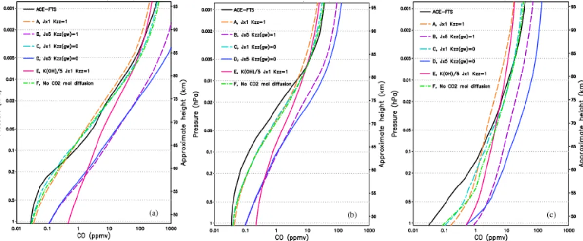
Similar to Fig. 5, Fig. 8 shows profile data for ACE and CMAM CO at latitudes where there is adequate data, 30◦N, 3◦N and 80◦S respectively. The CMAM data are for the scenarios listed in Table 1. The standard CO profile is in reasonable agreement with the

20

ACE data below 0.01 hPa (∼80 km); above this height it is lower than the observations and is 30% too low by 1.10−4hPa (∼98 km) for these latitudes. Case B with increased photolysis is too large by a factor between 4 and 5, varying with height. Given that the model CO₂ is in reasonable agreement with the observations for this case, this suggests that the CO source is too large by about a factor of 5. This strongly suggests

25

that increased photolysis cannot solve the problem and is thus an important constraint. Scenario C with decreased KZ Z is in reasonable agreement with the observations (but

(14)

ACPD

9, 11551–11587, 2009

Title Page

Tables Figures

◭ ◮

Back Close

Full Screen / Esc

the worst case and the disagreement of scenario B is amplified by the reduction of downward di_ffusion due to K_{Z Z}. For scenario E the VMRs reflect the slower CO loss rate so that the model mixing ratios are too large below about 0.005 hPa (∼85 km). The effect of zeroing molecular diffusion for CO₂ (scenario F) increases CO due to larger VMRs of CO₂ in the lower thermosphere. For the tropics the comparison is similar.

5

Scenarios B and D produce CO mixing ratios that are much too large compared to the ACE observations. The other scenarios are generally too low above about 80 km. For the austral polar region, similar behaviour is exhibited as for the other latitudes. It should be noted that none of the model results give agreement below 0.1 hPa (∼70km) and the standard run is too small by a factor of 2 at∼0.001 hPa (∼92 km).

10

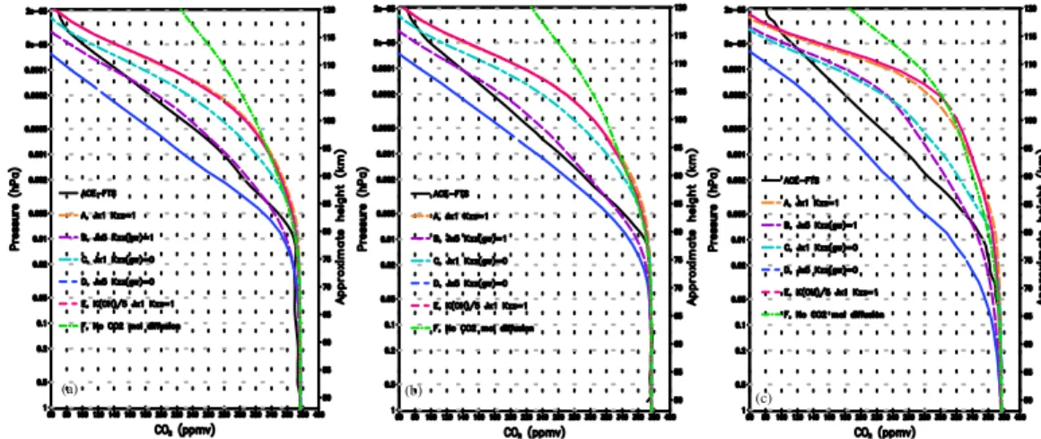
The above has focused on vernal equinox. We now investigate the late northern summer, August, to ensure that the same characteristics prevail for all seasons. August is a month where the ACE data has adequate coverage from the northern sub-tropics to the austral polar regions. Figure 9 shows the ACE CO₂ data for August and the CMAM data for the scenarios discussed above and shown in Table 1 (scenario E is

15

not included for August). A comparison of the ACE data with the standard scenario, A, shows that the behaviour is similar in August as for April in that the measured CO₂ begins to fall o_ff at lower altitudes than does the model. We note that the slopes of the ACE contours in the polar region are affected by sampling as for April as can also be seen in Jin et al. (2008). However, there are qualitative differences between April

20

and August for the other scenarios. For example, scenario B with an increased J value is now excessive, in that the CMAM CO₂ falls offtoo rapidly in this case. Scenario C with K_{Z Z}(GWD) turned offproduces results where CO₂is too high while for scenario D, the combination of B and C, CO₂is excessive as for the April results. And scenario F with molecular diffusion turned offclearly shows the importance of molecular diffusion.

25

We have also looked at the plots (not shown) for specific latitudes as for April and the above behaviour is confirmed.

(15)

ACPD

9, 11551–11587, 2009

Title Page

Tables Figures

◭ ◮

Back Close

Full Screen / Esc

0.05 hPa (∼75 km) but is about a factor of 2 low at 0.001 hPa (∼92 km) and the latitudi-nal behaviour is quite similar. For scenario B, the CO is generally too high by up to a factor of five which again suggests that an increased J value is not the solution for the poor fit for the control. Scenario C with a decreased K_{Z Z} leads to an even poorer fit at∼0.001 hPa as the CO is not di_ffused down as rapidly while the agreement remains

5

reasonable at∼1 hPa since the distribution is controlled by chemistry. Scenario D is, as expected, poorer than either B or C. Similar to the results for April, case F gives reasonable CO concentrations in the upper part of the domain that, however, reflects unrealistically high CO₂concentration in the lower thermosphere.

5 Discussion

10

As far as we can discern this is the first published 3-D study of CO₂in the MLT region using a GCM with a vertical domain that extends from the surface to the thermosphere. As noted above, Kaufmann et al. (2002) presented a 3-D study of CO₂using the TIME-GCM. This is a 3-D time dependent GCM extending from 30 to 500 km, and for their cal-culations they used a 5◦×5◦ horizontal resolution with two grid points per scale height

15

in the vertical and a 4 min time step (see for example Roble (1995) and references therein for a more detailed description for the TIME-GCM). Kaufmann et al. (2002) found problems, similar to what we have elucidated above, with the di_fferences of the vertical distributions of CO₂mixing ratio between measurements and model. Mertens et al. (2008) find similar discrepancies between the SABER V1.06 CO₂profiles and the

20

TIME-GCM. Chabrillat et al. (2002) have used a 2-D model to investigate the impact of molecular diffusion on the CO₂ distribution in the MLT region. They obtained reason-able agreement with the rocket measurements but did not explicitly compare with the CRISTA measurements which have a knee much lower.

The figures presented above explore a series of sensitivity tests to examine the

ma-25

(16)

sig-ACPD

9, 11551–11587, 2009

Title Page

Tables Figures

◭ ◮

Back Close

Full Screen / Esc

nificantly, far beyond any reasonable uncertainty in the known parameters determining the photolysis in this region. Other factors such as the magnitude of turbulence gener-ated by breaking of the unresolved gravity waves, uncertainties in the CO₂reformation rates and the action of molecular diffusion at this altitude seem unable to produce the correct change in distribution of the CO₂. We note that the application of K_{Z Z}(GWD) is

5

not a standard feature of middle atmosphere models. To our best knowledge, there are only two GWD parameterizations (Hines, 1997a,b; Lindzen, 1981) which provide eddy di_ffusion coe_fficients. That is why we have investigated the impact of K_{Z Z}(GWD) re-moval. In addition, the resolved circulation in the middle atmosphere is quite sensitive to the tuning of GWD parameterizations and this can also affect the species distribution

10

as much as K_{Z Z}(GWD). Given the uncertainty in our knowledge of the e_ffects of di_ff u-sion generated by gravity wave breaking, a major contributor to the K_{Z Z} in this region, some concern over the role and strength of gravity wave induced motion is warranted. However, even if we neglect all di_ffusive transport associated with unresolved gravity wave breaking, the CO₂ vertical profile does not begin to fall o_ffin the model as low

15

as the ACE observations indicate. Nevertheless we note that for other species in the MLT region, such as H₂O, N₂O, CH₄, as well as CO₂, for which their distributions are determined by vertical transport balanced by chemical loss, that knowledge of K_{Z Z} is important in the determination of their distributions (see also Jin et al., 2008).

Although the photolysis rate of CO₂appears reasonably well characterized, except,

20

as noted above, at longer wavelengths, we have estimated what increase might be required to produce agreement (without consideration of CO): this is scenario B. This scenario appears to be the only simulated process capable of reconciling the model and observations amongst the scenarios considered. Although, based on the current knowledge, we could not find any physical reasons for the CO₂ photolysis to be a

25

few times larger than that used in scenario A; results from scenario B clearly indicate that some additional CO₂ loss processes are required in the mesosphere in order to reconcile the model and observations.

(17)

0.1-ACPD

9, 11551–11587, 2009

Title Page

Tables Figures

◭ ◮

Back Close

Full Screen / Esc

1.10−4hPa), the CO₂ molecule is photolyzed mainly in the Lyman-α line. In this case the value of the photolysis rate depends on CO₂ and O₂ cross sections in the vicin-ity of Lyman-α and on the level of solar activity. The solar flux in the Lyman-α line varies by about 30% from solar maximum to solar minimum. However, for the pe-riod of the ACE observations (2004–2007), the solar irradiance at Lyman-α line

re-5

ported on the SOLARIS website (http://www.geo.fu-berlin.de/en/met/ag/strat/research/ SOLARIS/Input data) does not di_ffer by more than 10% from that used in our calcula-tion, with our value being generally larger.

The CO₂ cross section at Lyman-α for about 300K reported by di_fferent authors varies between (6.5–8.2)×10−20cm2 (e.g. see Yoshino et al., 1996). There is also a

10

weak temperature dependence: the cross section slowly increases with temperature at 0.1%/K (Lewis and Carver, 1983). Some uncertainties exist in what temperature the cross section should be taken at. The kinetic temperature in the upper mesosphere is generally lower than 200K. However, there is some justification for higher temperatures being used. This is because the vibrational levels of CO₂are non-thermally excited in

15

the mesosphere so that daytime vibrational temperatures are higher than the kinetic temperature (e.g., L ´opez-Puertas and Taylor, 2001). However, this cannot likely explain a considerable increase in the CO₂ photolysis rate. Daytime vibrational temperatures do not exceed 250 K and 350 K for the lower and higher vibrational levels, respectively (e.g., L ´opez-Puertas and Taylor, 2001). Given the temperature dependence of the

20

CO₂ cross section to be 0.1%/K, the latter means that non-thermal excitation of the CO₂vibrational levels cannot lead to a cross section increase of more than∼5% from the value measured at 300 K.

Chabrillat and Kockarts (1997) have noted that because of the structure in the O₂ absorption cross section in the vicinity of Lyman-α that J values for H₂O and CH₄ are

25

(18)

ACPD

9, 11551–11587, 2009

Title Page

Tables Figures

◭ ◮

Back Close

Full Screen / Esc

et al., 2003; Shemansky, 1972; Karaiskou et al., 2004). However this long wavelength uncertainty should only a_ffect J(CO₂) for altitudes below about 65 km (∼0.2 hPa) (see, for example, Brasseur and Solomon, 1984) and not impact our calculations. For the CO₂ cross section in the Lyman-α region we use a value of 7.7×10−20cm2 which suggests that even with all the uncertainties taken into account, we rather overestimate

5

the CO₂photolysis rate in the upper mesosphere than underestimate it.

CO provides an important additional constraint on the problem of the carbon distri-bution in the MLT region. CO is created from the CO₂photolysis and is advected and diffused from above. In the control model simulation, scenario A, CMAM CO is up to a factor of two too low above∼0.01 hPa (∼80 km) but it is not clear how serious a

dis-10

agreement this is. But even though the source, CO₂, is too high and the J value should be appropriate the CO is low. As noted above there is no clear evidence to suggest a serious error in the photolysis rate of CO₂at these altitudes. A number of the sensitivity experiments do create higher CO levels at the pressure range required to mimic the ACE observations, viz., scenarios B (enhanced photolysis of CO₂), C (reduced K_{Z Z}),

15

and F (molecular diffusion=0) as can be seen from Figs. 7 and 8. A change in K_{Z Z} could be envisaged to get CO closer to the ACE observations but a neglect of molec-ular di_ffusion (namely no gravitational separation of CO₂) is physically unreasonable. And, as we have seen in Figs. 7, 8 and 10, the J value enhancement results indicate that the concomitant increase in CO is too large compared to the ACE observations.

20

For this scenario B the agreement between measured and modelled CO has worsened above 65 km with the source of CO having increased dramatically and unrealistically.

The impact of scenario C (K_{Z Z}(GWD)₌0) is to e_ffect a fall-o_ffin CO₂at lower altitudes as the upward transport of CO₂ down the mixing ratio gradient has been decreased. We note that the agreement between model and measurements is improved somewhat

25

(19)

ACPD

9, 11551–11587, 2009

Title Page

Tables Figures

◭ ◮

Back Close

Full Screen / Esc

for some species such as CO, NO, CH₄, N₂O, H₂O as well as CO₂ but its vertical and latitudinal structure has not been thoroughly explored. It would be interesting to investi-gate the impact of KZ Z fields derived from other GWD schemes. As noted above each

GWD scheme will induce not just a different dynamical and temperature structure but also a di_fferent species structure and by choosing suitable species it may be possible

5

to further constrain GWD parameterizations.

As is clear from above results the most reasonable scenario for agreement between the ACE observations and CMAM simulations is with an increased J value (perhaps with a different enhancement factor between April and August). However, the concomi-tant increased source of CO is not present in the observations. This is then suggestive

10

that carbon may be sequestered elsewhere in the atmospheric system. At this point our only suggestion is perhaps CO₂may react with meteoritic dust in the mesosphere. Es-timating reaction times at∼80 km using typical meteoritic surface areas (e.g., Megner et al., 2008) we obtain 9/γ hours where γ is the e_fficiency for non-reversible reaction on the dust, this should be compared with 1/J(CO₂) for Lyman-αat 80 km which is∼13

15

days for a diurnal average at mid-latitudes. Thus γ₌0.1 would yield a loss process

∼3–5 times faster than photolysis This could yield a faster CO₂removal rate while not producing CO. If this in fact proves to be the case then one might expect other similar reactions to be occurring on meteoritic dust. An interesting feature of such a phe-nomenon is that it will be sporadic, and its e_ffects will vary from season to season with

20

varying dust amounts which might account for the variation required in the “enhanced” J (CO₂) to account for the observations in April and August.

One of the issues that might be of importance to consider is how well the extended CMAM simulates temperatures. With this in mind we present zonally and temporarily averaged latitude-pressure temperature for ACE and the CMAM control run in Fig. 11a

25

(20)

ACPD

9, 11551–11587, 2009

Title Page

Tables Figures

◭ ◮

Back Close

Full Screen / Esc

6 Summary

We present the first global set of observations of ground state CO₂for the mesosphere and lower thermosphere. We also present the measurements of CO obtained concur-rently. They were obtained by the ACE-FTS instrument on SCISAT-I, a small Canadian satellite, using solar occultation. There are certain limitations on seasonal and zonal

5

averages due to the particular orbit which emphasizes investigations of polar regions and also due to the particular sampling properties of solar occultation. The CO₂mixing ratio distribution from ACE lies between the CRISTA values (Kaufmann et al., 2002) and the rocket values, (compilation by Fomichev et al., 1998), and is similar to the SABER V1.06 measurements (Mertens et al., 2009).

10

We have compared the ACE measurements to calculations of the CO₂and CO

dis-tributions using a version of the Canadian Middle Atmosphere Model (CMAM) which has been vertically extended to about 220 km. Applying standard chemistry we find that we cannot get agreement between the ACE observations and CMAM simulations in the mesosphere and in particular, the model cannot reproduce adequately the height

15

of the knee, i.e. the height at which CO₂ begins to fall o_ffwhile adequately reproduc-ing the CO observations. We have investigated the variation of several parameters of interest in order to explore parameter space for this problem. Our conclusions are that there must be a loss process for CO₂that will sequester the carbon in some form other than CO; we have speculated on the role of meteoritic dust. We also highlight

20

the important role for K_{Z Z}, viz. eddy diffusion of species associated with GWD.

Acknowledgements. The authors would like to thank the Canadian Space Agency (CSA), the

Natural Sciences and Engineering Research Council (NSERC) of Canada, the Canadian Foun-dation for Climate and Atmospheric Science (CFCAS), the Canadian FounFoun-dation for Innovation, the Ontario Innovation Trust for support and the UK Natural Environment Research Council.

(21)

ACPD

9, 11551–11587, 2009

Title Page

Tables Figures

◭ ◮

Back Close

Full Screen / Esc

References

Beagley, S. R., McLandress, C., Fomichev, V. I., and Ward, W. E.: The Extended Canadian Middle Atmosphere Model, Geophys. Res. Lett., 27(16), 2529–2532, 2000.

Beagley, S. R., McConnell, J. C., Fomichev, V. I., Semeniuk, K., Jonsson, A. I., Garcia Munoz, A., McLandress, C., and Shepherd, T. G.: Extended CMAM: Impacts of thermospheric

neu-5

tral and ion chemistry on the middle atmosphere, AGU, fall, 2007.

Bernath, P. F., McElroy, C. T., Abrahams, M. C., Boone, C. D., Butler, M., Camy-Peyret, C., Carleer, M., Clerbaux, C., Coheur, P.F., Colin, R., DeCola, P., DeMazire, M., Drummond, J. R., Dufour, D., Evans, W. F. J., Fast, H., Fussen, D., Gilbert, K., Jennings, D. E., Llewellyn, E. J., Lowe, R. P., Mahieu, E., McConnell, J. C., McHugh, M., McLeod, S. D., Michaud, R.,

10

Midwinter, C., Nassar, R., Nichitiu, F., Nowlan, C., Rinsland, C. P., Rochon, Y. J., Rowlands, N., Semeniuk, K., Simon, P., Skelton, R., Sloan, J. J., Soucy, M.-A., Strong, K., Tremblay, P., Turnbull, D., Walker, K. A., Walkty, I., Wardle, D. A., Wehrle, V., Zander, R., and Zou, J.: Atmospheric Chemistry Experiment(ACE): Mission overview, Geophys. Res. Lett., 32, L15S01, doi:10.1029/2005GL022386, 2005.

15

Boone, C. D., Nassar, R., Walker, K. A., Rochon, Y., McLeod, S. D., Rinsland, C. P., and Bernath, P. F.: Retrievals for the atmospheric chemistry experiment Fourier-transform spec-trometer, Appl. Opt., 44(33), 7218–7231, 2005.

Brasseur, G. and Solomon, S.: Aeronomy of the Middle Atmosphere, D. Reidel, 441 pp., 1984. Chabrillat, S. and Kockarts, G.: Simple parameterization of the absorption of the solar

Lyman-20

alpha line, Geophys. Res. Lett., 24, 2659–2662, 1997.

Chabrillat, S., Kockarts, G., Fonteyn, D., and Brasseur, G.: Impact of molecular diffusion on the CO2distribution and the temperature in the mesosphere, Geophys. Res. Lett., 29, 1729,

doi:10.1029/2002GL015309 2002.

de Grandpr ´e, J., Beagley, S. R., Fomichev, V. I., Griffioen, E., McConnell, J. C., Medvedev,

25

A. S., and Shepherd, T. G.: Ozone climatology using interactive chemistry: Results from the Canadian Middle Atmosphere Model, J. Geophys. Res., 105(D21), 26475–26492, doi:10.1029/2000JD900427, 2000.

Fomichev, V. I., Blanchet, J.-P., and Turner, D. S.: Matrix parameterization of the 15µm CO2

band cooling in the middle and upper atmosphere for variable CO2 concentration, J. Geo-30

phys. Res., 103, 11505–11528, 1998.

(22)

McFar-ACPD

9, 11551–11587, 2009

Title Page

Tables Figures

◭ ◮

Back Close

Full Screen / Esc

lane, N. A., and Shepherd, T. G.: Extended Canadian Middle Atmosphere Model: Zonal-mean climatology and physical parameterizations, J. Geophys. Res., 107(D10), 4087, doi:10.1029/2001JD000479, 2002.

Girard, A., Besson, J., Brard, D., Laurent, J., Lemaitre, M. P., Lippens, C., Muller, C., Vercheval, J., and, Ackerman, M.: Global results of grille spectrometer experiment on board Spacelab

5

1, Planet. Space Sci., 36, 291–300, 1988.

Hines, C. O.: Doppler-spread parameterization of gravity-wave momentum deposition in the middle atmosphere. Part 1: Basic formulation, J. Atmos. Sol.-Terr. Phys., 59, 371–386, 1997a.

Hines, C. O.: Doppler-spread parameterization of gravity-wave momentum deposition in the

10

middle atmosphere. Part 2: Broad and quasi-monochromatic spectra, and implementation, J. Atmos. Sol.-Terr. Phys., 59, 387–400, 1997b.

Jin, J. J., Semeniuk, K., Beagley, S. R., Fomichev,V. I., Jonsson A. I., McConnell, J. C., Urban, J., Murtagh, D., Manney, G. L., Boone, C. D., Bernath, P. F., Walker, K. A., Barret, B., Ricaud, P., and Dupuy, E.: Comparison of CMAM simulations of CO (CO), nitrous oxide (N2O), and 15

methane (CH4) with observations from Odin/SMR, ACE-FTS, and Aura/MLS, Atmos. Chem.

Phys. Discuss., 8, 13063–13123, 2008,

http://www.atmos-chem-phys-discuss.net/8/13063/2008/.

Jin, J. J., Semeniuk, K., Jonsson, A. I., Beagley, S. R., McConnell, J. C., Boone, C. D.,Walker, K. A., Bernath, P. F., Rinsland, C. P., Dupuy, E., Ricaud, P., De la Noe, J., Urban, J., and

20

Murtagh, D.: A comparison of co-located ACE-FTS and SMR stratospheric-mesospheric CO measurements during 2004 and comparison with a GCM, Geophys. Res. Letts, 32, L15S03, doi:10.1029/2005GL022433, 2005.

Karaiskou, A., Vallance, C., Papadakis, V., Vardavas, I. M., and Rakitzis, T. P.: Absolute ab-sorption cross-section measurements of CO2 in the ultraviolet from 200 to 206 nm at 295 25

and 373 K , Chem. Phys. Lett., 400, 30–34, 2004.

Kaufmann, M., Gusev, O. A., Grossmann K. U., Roble, R. G., Hagan, M. E., Hartsough, C., and Kutepov, A. A.: The vertical and horizontal distribution of CO2 densities in the upper

mesosphere and lower thermosphere as measured by CRISTA, J. Geophys. Res., 107(D23), 8182, doi:10.1029/2001JD000704, 2002.

30

Kaye, J. A. and Miller, T. L.: The ATLAS series of shuttle missions, Geophys. Res. Lett., 23, 2285–2288, 1996.

(23)

ACPD

9, 11551–11587, 2009

Title Page

Tables Figures

◭ ◮

Back Close

Full Screen / Esc

OH6= −→v v N6=₂ −→v v CO₂ (ν₃)−→O₂+hν(4.3µm) mechanism for 4.3-µm airglow, J. Geophys. Res., 83, 4743–4747, 1978.

Lewis, B. R. and Carver, J. H.: Temperature dependence of the carbon dioxide photoabsorption cross section between 1200 and 1970 A, J. Quant. Spectrosc. Radiat. Trans., 30, 297–309, 1983.

5

Lindzen R. S.: Turbulence and stress owing to gravity wave and tidal breakdown. J. Geophys. Res., 86, 9704–9714, 1981.

L ´opez-Puertas, M. and Taylor, F. W.: Non-LTE Radiative Transfer in the Atmosphere. World Scientific, Singapore/New Jersey/London/Hong Kong, 487 pp., 2001.

L ´opez-Puertas, M. and Taylor, F. W.: Carbon dioxide 4.3µm emission in the Earth’s

atmo-10

sphere: A comparison between NIMBUS 7 SAMS measurements and non-local thermody-namic equilibrium radiative transfer calculations, J. Geophys. Res., 94, 13045–13068, 1989. L ópez-Puertas, M., Zaragoza, G., L ópez-Valverde, M. Á., and Taylor, F. W.: Non local

thermo-dynamic equilibrium (LTE) atmospheric limb emission at 4.6µm 2, An analysis of the day-time wideband radiances as measured by UARS improved stratospheric and mesospheric

15

sounder, J. Geophys. Res., 103, 8515–8530, 1998.

McLandress, C., Ward, W. E., Fomichev, V. I., Semeniuk, K., Beagley, S. R., McFarlane, N. A., and Shepherd, T. G.: Large-scale dynamics of the mesosphere and lower thermosphere: An analysis using the extended Canadian Middle Atmosphere Model, J. Geophys. Res., 111, D17111, doi:10.1029/2005JD006776, 2006.

20

Megner, L., Siskind, D. E., Rapp, M., and Gumbel, J.: Global and temporal distribution of meteoric smoke: A two-dimensional simulation study, J. Geophys. Res., 113, D03202, doi:10.1029/2007JD009054, 2008.

Mertens, C. J., Winick, J. R., Picard, R. H., Evans, D. S., L ´opez-Puertas, M., Wintersteiner, P. P., Xu, X., Mlynczak, M. G., and Russell III, J. M.: Influence of solar-geomagnetic disturbances

25

on SABER measurements of 4.3µm emission and the retrieval of kinetic temperature and carbon dioxide, Adv. Space Res., 43, 1325–1336, 2009.

Mertens, C. J., Russell, J. M., Mlynczak, M. Y., She, C.-Y., Schmidlin, F. J., Goldberg, R. A., L ´opez-Puertas, M., Wintersteiner, P. P., Picard, R. H., Winick, J. R., and Xu, X.: Kinetic temperature and carbon dioxide from broadband infrared limb emission measurements taken

30

from the TIMED/SABER instrument, Adv. Space Res., 43, 15–27, 2009.

(24)

ACPD

9, 11551–11587, 2009

Title Page

Tables Figures

◭ ◮

Back Close

Full Screen / Esc

to spectral infrared rocket experiment data, J. Geophys. Res., 99, 10409–10419, 1994. Offermann, D. and Grossmann, K. U.: Thermospheric density and compositions as determined

by a mass spectrometer with cryo ion source, J. Geophys. Res., 78, 8296–8304, 1973. Offermann, D., Friedrich, V., Ross, P., and Von Zahn, U.: Neutral gas composition

measure-ments between 80 and 120 km, Planet. Space Sci., 29, 747–764, 1981.

5

Ogibalov V. P. and Fomichev, V. I.: Parameterization of solar heating by the near IR CO2bands

in the mesosphere, Adv. Space Res., 32, 759–764, 2003.

Parkinson, W. H., Rufus, J., and Yoshino, K.: Absolute absorption cross section measurements of CO₂ in the wavelength region 163–200 nm and the temperature dependence, Chem. Phys., 290, 251–256, 2003.

10

Philbrick, C. R., Faucher, G. A., and Trzcinski, E.: Rocket measurements of mesospheric and lower thermospheric composition, Space Res., 13, 255–260, Akademie, Berlin, Germany, 1973.

Remsberg, E. E., Marshall, B. T., Garcia-Comas, M., Krueger, D., Lingenfelser, G. S., Martin-Torres, J., Mlynczak, M. G., Russell III, J. M., Smith, A. K., Zhao, Y., Brown, C., Gordley,

15

L. L., L ´opez-Gonzalez, M. J., L ´opez-Puertas, M., She, C.-Y., Taylor, M. J., and Thomp-son, R. E.: Assessment of the quality of the Version 1.07 temperature-versus-pressure profiles of the middle atmosphere from TIMED/SABER, J. Geophys. Res., 113, D17101, doi:10.1029/2008JD010013, 2008.

Rinsland, C., Gunson, M. R., Zander, R., and L ´opez-Puertas, M.: Middle and upper atmosphere

20

pressure-temperature profiles and the abundances of CO2and CO in the upper atmosphere

from ATMOS/Spacelab 3 observations, J. Geophys. Res., 97, 20479–20495, 1992.

Roble, R. G.: Energetics of the mesosphere and thermosphere, the upper mesosphere and lower thermosphere: A review of experiment and theory, AGU Monograph, 87, 1995. Rothman, L. S., Jacquemart, D., Barbe, A., Benner, C. C., Birk, M., Brown, L. R., Carleer, M. R.,

25

Chackerian Jr., C., Chance, K., Coudert, K. H., Dana, V., Devi, V. M., Flaud, J.-M., Gamache, R. R., Goldman, A., Hartmann, J. -M., Jucks, K. W., Maki, A. G., Mandin, J. -Y., Massie, S. T., Orphal, J., Perrin, A., Rinsland, C. P., Smith, M. A. H., Tennyson, J, Tolchenov, R. N., Toth, R. A., Vander Auwera, J., Varanasi, P., and Wagner, G.: The HITRAN 2004 molecular spectroscopic database, J. Quant. Spectr. Radiat. Trans., 96, 139–204, 2005.

30

(25)

ACPD

9, 11551–11587, 2009

Title Page

Tables Figures

◭ ◮

Back Close

Full Screen / Esc

19, 3903–3931, 2006.

Schulz, C., Koch, J. D., Davidson, D. F., Jeffries, J. B., and Hanson, R. K.: Ultraviolet absorption spectra of shock-heated carbon dioxide and water between 900 and 3050 K, Chem. Phys. Lett., 355, 82–88, 2002.

Shemansky, D. E.: CO2Extinction Coefficient 1700–3000 ˚A, J. Chem. Phys., 56, 1582–1587, 5

1972.

Trinks, H. and Fricke, K. H.: Carbon dioxide concentrations in the lower thermosphere, J. Geo-phys. Res., 83, 3883–3886, 1978.

Yoshino, K., Esmond, J. R., Sun, Y., Parkinson, W. H., Ito, K., and Matsui, T.: Absorption cross section measurements of carbon dioxide in the wavelength region 118.7–175.5 nm and the

10

temperature dependence. J. Quant. Spectrosc. Radiat. Transfer, 55, 53–60, 1991.

Zaragoza, G., L ´opez-Puertas, M., L ´opez-Valverde, M. A., and Taylor, F. W.: Global distribution of CO2in the upper mesosphere as derived from UARS/ISAMS measurements, J. Geophys.

Res., 105, 19829–19839, 2000.

(26)

ACPD

9, 11551–11587, 2009

Title Page

Tables Figures

◭ ◮

Back Close

Full Screen / Esc

Interactive Discussion Table 1.Scenarios analysed.

Scenario Details

A-control KZ Z (GWD) included, standard rate constants and J values

B J(CO2) increased by a factor of 5 otherwise A

C KZ Z (GWD)=0, otherwise A

D B+C

(27)

ACPD

9, 11551–11587, 2009

Title Page

Tables Figures

◭ ◮

Back Close

Full Screen / Esc

Interactive Discussion Fig. 1. Zonally and monthly averaged ACE CO2 data (sunrise and sunset) for the period 21

(28)

ACPD

9, 11551–11587, 2009

Title Page

Tables Figures

◭ ◮

Back Close

Full Screen / Esc

(29)

ACPD

9, 11551–11587, 2009

Title Page

Tables Figures

◭ ◮

Back Close

Full Screen / Esc

Interactive Discussion Fig. 3. A comparison of mean rocket measurements (compilation by Fomichev et al., 1998),

global mean CRISTA observations (Kaufmann et al., 2002), daytime V1.06 SABER observa-tions (see text for details), global mean ACE measurements and global mean CMAM CO2.

(30)

ACPD

9, 11551–11587, 2009

Title Page

Tables Figures

◭ ◮

Back Close

Full Screen / Esc

Interactive Discussion Fig. 4. Zonally and monthly averaged latitude-pressure plots of CO2 volume mixing ratios

(31)

ACPD

9, 11551–11587, 2009

Title Page

Tables Figures

◭ ◮

Back Close

Full Screen / Esc

(a) (b) _(c)

Fig. 5. ACE CO2 profiles from Figure 4, for latitudes(a)30

◦

(32)

ACPD

9, 11551–11587, 2009

Title Page

Tables Figures

◭ ◮

Back Close

Full Screen / Esc

Pressure (hPa).

Approximate height (km).

Fig. 6. Latitudinal-pressure plot of KZ Z (GWD) in m 2

(33)

ACPD

9, 11551–11587, 2009

Title Page

Tables Figures

◭ ◮

Back Close

Full Screen / Esc

Interactive Discussion Fig. 7.Zonally and monthly averaged latitude-pressure plots of CO volume mixing ratios (ppmv)

(34)

ACPD

9, 11551–11587, 2009

Title Page

Tables Figures

◭ ◮

Back Close

Full Screen / Esc

(a) (b) (c)

(35)

ACPD

9, 11551–11587, 2009

Title Page

Tables Figures

◭ ◮

Back Close

Full Screen / Esc

Interactive Discussion Fig. 9. Zonally and monthly averaged latitude-pressure plots of CO2 volume mixing ratios

(36)

ACPD

9, 11551–11587, 2009

Title Page

Tables Figures

◭ ◮

Back Close

Full Screen / Esc

Interactive Discussion Fig. 10. Zonally and monthly averaged latitude-pressure plots of CO volume mixing ratios

(37)

ACPD

9, 11551–11587, 2009

Title Page

Tables Figures

◭ ◮

Back Close

Full Screen / Esc

Interactive Discussion Fig. 11. Zonally and monthly averaged latitude-pressure plots of temperature (K) for the ACE