Analysis in magnetic resonance elastography: study and development of image processing techniques

(1)

UNIVERSIDADE DE LISBOA

Faculdade de Ciências

Departamento de Física

Analysis in Magnetic Resonance Elastography: Study and

Development of Image Processing Techniques

Catarina Henriques Lopes dos Santos Rua

Dissertação

Mestrado Integrado em Engenharia Biomédica e Biofísica

Radiações em Diagnóstico e Terapia

(2)

(3)

UNIVERSIDADE DE LISBOA

Faculdade de Ciências

Departamento de Física

Analysis in Magnetic Resonance Elastography: Study and

Development of Image Processing Techniques

Catarina Henriques Lopes dos Santos Rua

Dissertação orientada pelos Prof. Doutores Marius Mada e

Alexandre Andrade

Mestrado Integrado em Engenharia Biomédica e Biofísica

Radiações em Diagnóstico e Terapia

(4)

Dedico a tese às minhas avós, Carminda dos Santos e

Maria Pereira Lopes.

Valeu a pena? Tudo vale a pena Se a alma nao é pequena. Quem quer passar além do Bojador Tem que passar além da dor. Deus ao mar o perigo e o abismo deu, Mas nele é que espelhou o céu. Fernando Pessoa, in Mensagem

(5)

v

Abstract

The term ―Elastography‖ unifies biomechanics with imaging sciences and was driven by the well-documented effectiveness of palpation as a diagnostic technique for detecting cancer and other diseases.

Notoriously, during the last decade Magnetic Resonance Elastography (MRE) has emerged as the most accurate imaging modality to non-invasively assess the rheological properties of tissue. Using a phase-contrast MRI technique together with an external mechanical actuation device, it is possible to detect propagating shear waves inside the human body. Viscoelastic properties can then be extracted by applying inversion methods to the acquired phase data. Due to the richness and significance of the data, and in spite of enduring challenges related to the complexity of the computations involved, MRE attracted strong interest and is now a thriving area of research.

The computations necessary to calculate maps of viscoelastic tissue properties are indeed substantial and are generally done on remote computers after completion of experiments. T he need for higher flexibility in large scale clinical studies led to the development, in the current project, of an automated toolbox for real time MRE data processing implemented within the scanner environment.

The most commonly used direct inversion methods, Algebraic Helmholtz Inversion (AHI) and Local Frequency Estimation, show considerable performance differences under similar initial conditions. Assumptions underlying such algorithms were studied by comparing noise sensitivity and resolution on synthetic, phantom and in vivo brain datasets.

Finally, a clinical application of the AHI approach was performed on brain and abdominal data from healthy individuals. The ensuing values of brain viscoelasticity suggest higher stiffness in white matter compared to grey matter. Preliminary results also show a pronounced age-related decrease in brain stiffness and viscosity. The liver, kidney and spleen were assessed with abdominal MRE and the results support a statistically significant higher stiffness in the spleen compared to liver and kidney.

Keywords: Magnetic Resonance Elastography, image processing, algebraic Helmholtz

(6)

vi

Resumo

A rigidez e viscosidade são das propriedades mecânicas intrínsecas dos tecidos com maior relevância fisiopatológica. Segundo as fontes conhecidas, desde 400 a.C., a palpação tem sido o método mais utilizado como primeira fonte de avaliação médica, de forma a detectar pequenas massas ou tumores em tecidos moles. No entanto, a experiência profissional do médico e a própria localização da massa têm um grande impacto na qualidade do diagnóstico efectuado.

Sabendo que o módulo de elasticidade possui uma variabilidade nos tecidos moles superior à de outras propriedades físicas, como a absorção de raios X ou o tempo de relaxamento em ressonância magnética nuclear, e que a ressonância magnética é das técnicas que, até à data, foi capaz de produzir imagens com maior qualidade e resolução espacial, surgiu uma forte motivação para unificar a biomecânica com a imagiologia por ressonância magnética.

Deste modo, a Elastografia por Ressonância Magnética (MRE, do inglês ―Magnetic Resonance Elastography‖) apareceu em meados dos anos 90 do século passado, permitindo avaliar e medir com um elevado grau de exactidão as propriedades reológicas dos tecidos, de modo não invasivo. Utilizando uma técnica de contraste de fase em MRI, em conjunto com um dispositivo dinâmico de oscilação mecânica, a MRE mostra um potencial muito grande para detectar a propagação de ondas mecânicas no corpo humano, com uma precisão da ordem de grandeza dos mícrons. Posteriormente à aquisição das chamadas ―imagens de fase‖, o processamento de imagem, através da aplicação de algoritmos de inversão, permite quantificar o comportamento reológico do meio.

Esta nova modalidade de diagnóstico deu até hoje lugar a um conjunto de estudos pré-clínicos que permitiram a investigação das condições mecânicas associadas a alterações fisiológicas e patológicas, em tecidos nos quais esta abordagem nunca tinha sido possível. Éntre esses tecidos, é de destacar o caso do cérebro, um órgão onde a palpação ou aplicação de elastrografia convencional, associada a ultrassons, é inviável devido à presença da caixa craniana. Podem-se, assim, enumerar alguns estudos empreendidos com esta técnica até hoje, de inquestionável impacto científico e clínico: a fibrose hepática, o envelhecimento do cérebro, a esclerose múltipla, a hidrocefalia e os tumores cerebrais.

Uma das áreas que actualmente atrai maior interesse consiste na correcta quantificação da viscoelasticidade a partir dos dados adquiridos no scanner. Tendo como base premissas diferentes, muitos algoritmos foram propostos para inverter a equação de ondas, calculando parâmetros relevantes a partir da simples propagação das ondas nos tecidos. Os métodos mais

(7)

vii intuitivos designam-se por métodos directos, sendo os mais comuns a Inversão Algébrica da equação de Helmholtz (AHI, do inglês ―Algebraic Helmholtz Inversion‖) e a Estimação da Frequência Local (LFE, do inglês ―Local Frequency Estimation‖). O primeiro tem por base uma origem matemática, realizando a inversão local em cada ponto da matriz da imagem segundo a equação de Helmholtz. A técnica de LFE, por outro lado, resolve o problema através de métodos de processamento, onde a aplicação de uma cadeia de filtros permite extrair a frequência espacial local das ondas de shear, estando esta relacionada com o módulo da elasticidade através de uma simples relação algébrica.

Neste contexto, a tese apresentada prende-se com os métodos de análise de imagem em MRE, nomeadamente tanto no estudo como no desenvolvimento de técnicas que permitem uma avaliação das propriedades dinâmicas do meio, com precisão, exactidão e flexibilidade.

Um dos problemas da baixa aplicabilidade da técnica de MRE a grandes estudos clínicos é, de facto, a falta de flexibilidade na obtenção de mapas de elasticidade. O volume de cálculos necessários para a construção desses mapas é muito grande, e por isso esses cálculos são geralmente efectuados em computadores independentes, depois de terminada a etapa da aquisição dos dados. Desta forma, o primeiro projecto consistiu no desenvolvimento de uma toolbox que permitisse o processamento de imagem em tempo real, embutido no proprio scanner. Assim, aquando da aquisição de uma experiência de elastografia, será possível obter não só a disposição espacial e intensidade da propagação das ondas mecânicas, mas também um mapa adicional correspondente à elasticidade do tecido, directamente na sala de controlo. Para este efeito, foi desenvolvido um algoritmo de reconstrução codificado num ambiente compatível com o sistema de computação de scanners da Siemens. Depois de várias fases de avaliação, desenvolvimento, debugging e validação do algoritmo, tanto offline como inline em simuladores, foram realizados testes no próprio scanner em fantomas e no cérebro de um voluntário saudável, utilizando várias frequências de oscilação. Desta forma, pôde-se verificar o sucesso global da toolbox implementada. Ainda assim, será necessária uma fase de optimização no sentido de criar uma toolbox de uso mais familiar e melhorar o algoritmo em si, corrigindo alguns problemas da versão actual.

Os dois algoritmos de reconstrução mais utilizados a nível clínico, AHI e LFE, anteriormente apresentados e contextualizados, revelam um desempenho surpreendentemente diferente, sob condições iniciais idênticas e não obstante os princípios físicos subjacentes serem semelhantes. Estas inconsistências reflectem-se numa vasta gama de valores para o módulo de elasticidade verificados na literatura. Por conseguinte, foi efectuado um estudo para testar a qualidade das reconstruções em termos de sensibilidade, resolução espacial e eficácia na reconstrução em fantomas gerados sinteticamente, onde ruído, atenuação, ondas de compressão e padrões de interferência foram adicionados a uma equação de ondas básica.

(8)

viii Para avaliar o desempenho dos algoritmos em dados de MRE extraídos do scanner, utilizaram-se jogos de dados obtidos com fantomas de gel sem e com inclusões de elasticidade dissemelhante entre regiões, assim como dados cerebrais de indivíduos saudáveis. Em geral, os resultados demonstram que o método LFE é mais eficaz em condições ideais, mas carece de precisão na análise de imagens sintéticas com artefactos tal como em dados reais. Isto é devido essencialmente a uma filtragem excessiva, assim como ao facto de o algoritmo não considerar a atenuação como uma premissa do modelo. Pelo contrário, os mapas obtidos pelo método AHI são mais nítidos mas são altamente susceptíveis a ruído. Mais se concluiu, que certas metodologias que antecedem a inversão são de extrema importância, destacando -se o processo de filtragem espacial. Finalmente, a medição das propriedades físicas dos fantomas através de reometria convencional permitiu verificar uma disparidade nas duas técnicas, podendo levar à conclusão de que as reconstruções obtidas em MRE são sobrestimadas. No entanto, deve ser efectuada uma análise mais profunda em condições experimentais tão idênticas quanto possível, para que se possam confirmar estes efeitos.

O método AHI foi escolhido para estudar o cérebro de nove indivíduos saudáveis com idades compreendidas entre os 19 e os 62 anos. Neste estudo foram identificadas diferenças significativas, tanto na elasticidade como na viscosidade da matéria branca e cinzenta em todos os indivíduos, constatando-se que a última é a menos rígida. Além disso, um modelo linear regressivo foi ajustado aos valores obtidos com o método AHI tendo em conta a idade do sujeito, de forma a verificar tendências relativas esta variável. Resultados preliminares evidenciam uma distribuição linear com um declive negativo indicativo de um decréscimo pronunciado da elasticidade do tecido cerebral com a idade: a percentagem de decréscimo anual previsto foi de 0,75%. Apesar de não ser estatisticamente significativo, foram ainda identificadas pequenas diferenças nas taxas de decréscimo da elasticidade e viscosidade da matéria branca e cinzenta. No entanto, os resultados obtidos fazem parte de um estudo em curso e, como tal, será necessário testar um amostra superior para confirmar os resultados mencionados, assim como métodos mais sofisticados para analisar os dados.

Por fim, realizou-se um estudo sobre as propriedades viscoelásticas de tecidos do abdómen. Sendo a sequência utilizada baseada em ―Echo Planar Imaging‖ (EPI), as inomogeneidades do campo magnético e artefactos de ghosting são mais pronunciados na aquisição de imagem em tecidos moles no abdómen. Foi necessário assim, numa primeira fase, optimizar o protocolo de aquisição: o uso de bandas de saturação para suprimir o tecido adiposo, ajustes no ‖Field of View‖, o uso de técnicas de shimming e aquisição de imagem apenas durante apneia expiratória. O dispositivo que permite a distribuição de propagação das ondas nos tecidos também foi explorado, de forma a obter uma propagação uniforme com elevada amplitude ao longo da totalidade do corte. A aquisição de dados de cinco voluntários

(9)

ix saudáveis permitiu avaliar três tecidos com níveis de elasticidade distintos: o fígado, os rins e o baço. As principais conclusões retiradas indicam que o fígado e rins apresentam uma elasticidade menor que o baço, sob o modelo linear de tensão-deformação no qual se baseia o método AHI. Ainda assim, todo o processo de optimização está longe de se dar por concluído, pretendendo-se obter uma reprodutibilidade entre experiências com um protocolo de implementação expedito para ser possível aumentar a quantidade de dados e fazer uma análise estatística com um nível de confiança superior.

Em conclusão, a técnica de MRE mostra um enorme potencial para detectar alterações na elasticidade dos tecidos através de pequenas deformações periódicas induzidas durante a aquisição de imagem numa ressonância magnética. A tese apresentada aborda pontos importantes relativos à fase do processamento e análise de dados, contribuindo para a evolução da MRE no sentido da aceitação desta técnica em ambiente clínico. Soluções concretas para uma análise rápida a tempo real foram dadas através do desenvolvimento da

toolbox. Numa outra perspectiva, foram estudados nesta tese aspectos técnicos relevantes

relativos aos algoritmos de inversão, críticos para a obtenção de um processamento profundo e correcto dos dados obtidos. Por fim, os trabalhos desta tese resultaram na identificação e reconhecimento de diferenças entre a viscoelasticidade dos tecidos, medida in vivo, a um nível pré-clínico, deixa em aberto todo um conjunto de ideias para estudos inovadores na área da biomecânica aplicada ao ser humano em conjunção com imagiologia

Palavras-Chave: Elastografia por Resonância Magnética, processamento de imagem,

(10)

x

Acknowledgments

A year in Cambridge with a life changing experience. This thesis reflects not only my work, but also the help and support of special people without whom this would never have been possible.

First and foremost, I would like to thank my supervisor, Dr. Marius Mada, for all the effort and guidance given, and specially for being my friend. I would not be where I am without you. A special thanks to Dr. Guy Williams, for the patience you had with my endless problems with the code. I am also grateful to my second supervisor, Dr. Alexandre Andrade, for all the insightful advice throughout the thesis.

I thank Dr. Adrian Carpenter and all the people at the WBIC for accepting me and providing a great work environment every day. I would like to acknowledge the MRE groups from Charité in Berlin and from CRIC in Edinburgh for all the help you gave us to set-up MRE at the WBIC. And to all the volunteers that spared their time to have us shake their brains and livers, a huge thank you.

A great thanks Joana for being my friend, co-worker and wonderful MRE volunteer, personal advisor, cooking buddy, travelling partner, etc etc etc. When tough times came, you still believed in me, thanks for not letting me go. Also to Rafael, our DTI geek at home, I will never forget our friendship.

A very special thanks to Carolina, Inês and Marco who make my life happier like no others can. A skype call is all it takes.

And finally, the deepest thanks to my parents and my brother. Throughout my 23 years I recognize and truly appreciate the unconditional support you gave me on so many levels. Obrigada por tudo.

(11)

xi

List of Tables

Table 5.1. Viscoelastic constants determined by the Springpot, Zenner, Maxwell and Voigt fits for the homogeneous phantoms 1:3, 1:2, and 1:1. ... 67 Table 6.1. Isotropic lower and upper threshold wavelengths used on the spatial Butterworth band pass filter for brain experiments. ... 76 Table 6.2. Mean (standard deviation) G’ and G’’ results obtained from the brain experiments to assess WM and GM elasticity. These values originate from a mean over all subjects. For each subject, the mean G’ & G’’ value over the 5 slices was taken. ... 79 Table 6.3. Extracted model coefficients for brain, and white and gray matter, separately. ... 80 Table 6.4. Isotropic lower and upper threshold wavelengths, in mm, used on the spatial band pass filter for liver experiments. ... 85 Table 6.5. SNR values of the different phantom structures without (w/o) and with the fat bands. (SNR=mean/std). ... 89 Table 6.6. Literature and present results of liver viscoelasticity using different analysis methods. 98

(15)

xv

List of Figures

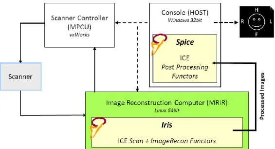
Figure 2.1. (a) The stress principle demonstrated on a body B with random form. The section is exerting a positive force, , on the negative side of the normal . (b) Representation of normal and shearing stresses on three sides of a cubic body. ... 5 Figure 2.2. Patterns of deformation on different shapes. ... 6 Figure 2.3. Deformation of a body. ... 6 Figure 2.4. Stress-strain curves for a pure elastic material (a) and a viscoelastic material (b). The blue area is the hysteresis loop, showing the amount of energy lost in loading and unloading. ... 8 Figure 2.5. Three mechanical models of viscoelastic material. (a) Maxwell body, (b) Voigt body, (c) Kelvin body (a standard linear solid) and (d) Springpot body. ... 10 Figure 3.1. Typical MRE experiment on a human brain to illustrate the different processes: motion generation, wave image acquisition and image processing. Adapted from [37]. ... 18 Figure 3.2. Loudspeaker systems for vibration generation in MR Elastography. (a) MR-Touch: this system has an active driver outside the magnet room and generates alternating pressures at a controlled frequency. The air is transmitted by a tube to a passive driver at the skin surface [23]. (b) Head cradle unit and mechanical wave generator to be positioned inside the magnet room for studies in the brain [33]. ... 19 Figure 3.3. (a) Brain and (b) liver MRE setups using the piezoelectric actuation device. ... 20 Figure 3.4. CAD design of the piezoelectric actuator which is mounted on the MRI bed at the patient’s feet in (a) the brain and (b) liver setups. The blue arrows indicate the direction of motion. ... 21 Figure 3.5. Pulse sequence diagram. The trigger pulses are synchronized with the motion encoding gradient (MEG), such that the frequency and number of gradient cycles N of the MSG is variable. ... 21 Figure 3.6. Configuration of the optimal gradient encoding vector G in respect to the displacement vector u. ... 24 Figure 4.1. MRE-Touch interface for post-acquisition processing on a General Electric (GE) MR host computer machine... 28 Figure 4.2. A simplistic version of the ICE workflow on a Siemens MR scanner. ... 30 Figure 4.3. Workflow of the Simulation Environment for an ICE programme. Adapted from [53]. 30

(16)

xvi Figure 4.4. GUI screenshots of the offline Matlab-based MRE processing toolkit (a) in processing phase and (b) the final results. ... 34 Figure 4.5. Block diagram of the MRE processing C++ code structure. ... 35 Figure 4.6. A basic diagram block of the inline processing with the ICE wrapper. The MREProcess Functor includes the code that will be added to normal the image acquisition and storage pipeline. ... 37 Figure 4.7. (a) Raw images of six phase off-sets of the homogeneous phantom at 100 Hz excitation frequency. (b) Unwrapped images after the application of the Flynn’s approach. .... 39 Figure 4.8. Temporal Fourier transformation technique. Image maps of f=0Hz, and the first and second harmonics after tFFT. Most of the energy is accumulated of the first harmonic. ... 39 Figure 4.9. Filtering process of the AHI algorithm implemented in C++. (a) k-space of the 1st

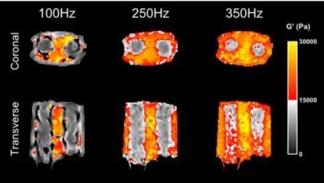
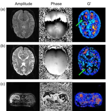
harmonic; (b) application of the k-space shift; (c) k-band of the spatial 4th order butterworth band-pass filter; (d) application of the filter in (c) to the k-space in (b); (e) result after he fftshift routine changing higher frequencies to the image limits and lower frequencies to the image centre. ... 40 Figure 4.10. Results of filters with different low-cut (lc) and high-cut (hc) wavelengths, in mm, on the cylinder phantom excited at 200 Hz. (a) lc=10.8 & hc=27.7; (c) lc=6.67 & hc=200; (c) lc=11.1 & hc=12.5; (d) lc=25.0 & hc=50.0. ... 41 Figure 4.11. N-G Laplacian directional terms ( on the left and on the right) computed with the (a) matlab and (b) C++ codes. ... 41 Figure 4.12. G’ map before and after application of the median smoothing filter with a window of 3x3 pixels with (a) Matlab implementation (c) C code implementation. ... 42 Figure 4.13. Single slice of a homogeneous phantom 1:3 (gelatine:water) excited at 200 Hz vibration frequency. (a) Unwrapped and filtered wave image at excitation frequency acquired with Matlab. (b) Matlab processed G’ result; (c) G’ result of the C++ code compiled on a Linux system (c) G’ result obtained with the ICE simulator. ... 42 Figure 4.14. A two cylinder inclusion phantom with 1:1 background and 1:2 cylinder inclusion stiffnesses. Results obtained with the real time MRE toolbox acquiring coronal and transverse slices. ... 43 Figure 4.15. MRE Experiments on brain using the real-time processing toolbox for MR Elastography. (a) Overall view of the scanner and host computer showing three computed frequency dependent G’ maps. (b) Detail of the sequence descriptions. . 44

(17)

xvii Figure 4.16. Real time MRE results performed on a healthy brain at three different driving frequencies acquired over 5 slices... 45 Figure 4.17. (a) Original amplitude and phase brain data at 25 Hz and its processed G’ map. Zero valued regions pointed by green arrow indicate spurious results from to the algorithm itself. (b) Amplitude and phase brain data at 37.5 Hz. Green arrow points to zero-valued regions in the real time computed G’ map, showing that automatic ROI was not performed correctly. (c) Amplitude and phase of a liver scan, with corresponding colour G’ map. ... 45 Figure 4.18. Estimative of the relative processing time between Matlab and the C++ codes. ... 46 Figure 4.19. Screenshot of the MRE-EPI sequence special card to configure specific parameters for acquisition. ... 48 Figure 5.1. (a) Example of a gel phantom sample used in rheometer tests; (b) ARES controlled strain rheometer; (c) BOHLIN controlled stress rheometer. ... 53 Figure 5.2. Approximated imaging region of the 5 slices in the brain for planar MRE. ... 54 Figure 5.3. Noise induction simulations. First phase offset from phantoms with (a) 10%, (b) 50% and (c) 90% Gaussian noise. Resultant G’ maps are represented in the two rows below ((d)-(i)), comparing no filter, left, with the application of a pre-inversion filter on the right (low-cut wavelength = 0.0109 m). ... 55 Figure 5.4. Spatial mean phase velocity results for the simulated software phantom at 50 Hz mechanical frequency, cp=1.45 m/s with increasing Gaussian noise corruption levels

from 1 to 100%. Measurements in green and light blue result from AHI and LFE inversions, respectively, with pre-filtering: low-pass filter with low-cut wavelength of 10.9 mm. The expected result is represented by the dashed black line. ... 56 Figure 5.5. Damping effects evaluation on software phantoms with wave motion at different frequencies (25.0, 37.5, 50.0, 62.5 and 75.0 Hz). Top row represents the first phase offset, the middle row shows the G’ maps estimated by AHI inversion, and the bottom row shows the G’ reconstructions using the LFE method. The green dashed line represents the profile direction for Figure 5.6 and Figure 5.7. ... 57 Figure 5.6. G’ estimation along the direction of motion propagation at 5 driving frequencies (25.0, 37.5, 50.0, 62.5 and 75.0 Hz) using: (a) the AHI inversion method and (b) the LFE method. In (c) the G’’ profile from AHI inversion was obtained which suggests the damping effects along the direction of motion propagation. ... 57 Figure 5.7. Evaluation of software phantom at 50 Hz driving frequency and phase velocity of 1.45 m/s. The phase velocity of the Gaussian envelopes were varied from 0.6 to 1.4 m/s. (a) Result of the wave propagation along the direction of motion with the application of the envelopes. (b) Profile of G’ maps estimated using the AHI inversion technique.

(18)

xviii (c) Profile of G’ maps estimated using the LFE inversion technique (a close-up of the first 45 pixels is also shown in the smaller graph). ... 58 Figure 5.8. Simulation of phantoms with shear wave propagation at 50 Hz in an elastic medium (cp=1.45 m/s) with added compressional interference waves (cp=1.20 m/s; freq = 0-25

Hz). The plot shows the mean phase velocity over the FoV estimated with AHI and LFE methods. Lines in red and light blue represent results with pre-inversion high-pass filtering: filter cut-off wavelengths according to each longitudinal frequency were, respectively, 0, 0.20, 0.11, 0.07, 0.05 and 0.04 m. The expected result is represented by the discontinued black line. ... 59 Figure 5.9. Three examples of high-pass spatial filter corrections on simulated phantoms with 50 Hz wave propagation, phase velocity of 1.45 m/s, and added compressional waves with the following characteristics: (a) 25 Hz, cp=1.20 m/s; (b) 30 Hz, cp=1.20 m/s; (c)

25 Hz, cp=1.20 m/s and an additional π/4 dephasing component. Respective G’ maps

for AHI and LFE inversions are shown on two columns on the right. ... 60 Figure 5.10. Simulated software phantoms with different directional wave components. (a)-(d) show the phase images and white arrows represent the relative amplitude and direction vectors of each wave component. Example of results for (e) AHI and (f) LFE inversions from the above phase images. (g) Spatial mean phase velocity results estimated for AHI and LFE methods for each of the tested phantoms. ... 61 Figure 5.11. Simulated software phantom with two oblique wave components (a) and (b) (wave vectors represented in white). (c) Resulting phase offset; (d) y-axis profile of the phase offset (red) and two diagonal components (blue and green) taken in the position represented by the discontinued white line. (e) and (f) are G’ results of the AHI and LFE inversions, respectively. ... 61 Figure 5.12. G’ variations with filter type for the homogeneous phantom at 50, 100, 200, 250 and 350 Hz. Spatial mean values were obtained from an ROI covering the field of view of the phantom. Low-cut wave numbers were chosen with the following values at the 5 increasing driving frequencies, respectively: 70, 90, 150, 170 and 200 m-1. ... 62 Figure 5.13. Homogeneous 1:3 phantom at 200 Hz excitation frequency. (a) Top row represents the complex wave images after temporal FFT. The values on top are the high-cut wavelengths used in the spatial filter. The bottom row shows reconstructions using AHI algorithm from the respective filtered wave images. (b) SNR variations with the high-cut wavelength calculated from the reconstructed maps (SNR=mean/standard deviation). ... 62 Figure 5.14. Filter variations with the type of algorithm used for reconstructions on the homogeneous phantom. lc and hc represent the lower and upper bounds, in mm, of the 4th order Butterworth band pass filter. ... 63

(19)

xix Figure 5.15. Cylinder phantom at 200 Hz excitation frequency. (a) T2-weighted magnitude image; (b) real part of the complex wave image; (c)-(e) reconstructed elasticity maps using the AHI N-G, AHI S-G and LFE methods, respectively; (f) plot of image profiles of the expected G’ and what was obtained with the 3 reconstructed maps; (g) image profiles for the AHI S-G algorithm varying polynomial orders and pixel window lengths. ... 64 Figure 5.16. Spatial mean G’ values determined using different computational algorithms in ROIs placed both in the background and cylinder at 100, 200, 250 and 350 Hz mechanical frequency stimulations. ... 64 Figure 5.17. Amplitude sweeps of the homogeneous phantoms (a) 1:1, (b) 1:2 and (c) 1:3 at 10rad/s. The limit of linear viscoelastic behaviour of the samples is marked by the black dashed line on each graph. ... 65 Figure 5.18. Viscoelastic model fits to 1:1 homogeneous phantom on rheology data. G’ results are shown in blue and G’’ results in red. MRE data is represented in black. ... 66 Figure 5.19. Springpot fits on rheometer measurements of the three types of homogeneous phantoms: (a) 1:3, (b) 1:2; (c) 1:1. G’ results are shown in blue and G’’ results in red, while MRE data is presented in black markers. ... 66 Figure 5.20. Viscoelastic model fits on rheology data for PDMS. G’ results are in blue and G’’ results in red. ... 67 Figure 5.21. Bohlin rheometer measurements on the 1:1, 1:2, 1:3 homogeneous phantoms with springpot fit to the datasets. G’ results are shown in blue and G’’ results in red. MRE results are also represented in black symbols. Rheometer measurements inside the black dashed line are compromised. ... 68 Figure 5.22. Rheometer stability: (a) ARES and (b) BOHLIN. The dashed lines represent the frequency band in which the performance of the rheometer is not compromised. .. 68 Figure 5.23. (a) Real part of the complex wave amplitude maps of one volunteer after temporal Fourier transformation at the 5 driving frequencies. The images were scaled according to the factors shown on the bottom right corner. (b) and (c) represent the reconstructed maps using the AHI and LFE algorithms respectively. ... 69 Figure 5.24. Mean and standard deviation G’ results obtained from the brain experiments using the AHI and LFE processing schemes. These values originate from an average over all subjects. For each subject, the mean G’ value over the 5 slices was taken. ... 69 Figure 5.25. Filter variations with the type of algorithm used for reconstructions in brain. lc and hc represent the lower and upper bounds, in mm, of the 4th order Butterworth band-pass filter. ... 70

(20)

xx Figure 6.1. MRE data processing of a single subject at six vibration frequencies (25, 37.5, 50, 62.5, 75 and 100 Hz). (a) Wave displacement in microns, scaled according to the factors shown on the bottom right corner. The images were scaled according to the factors shown on the bottom right corner. (b) G’ estimation with AHI algorithm; (c) segmented white matter G’ maps; (d) segmented grey matter G’ maps. ... 77 Figure 6.2. (a) G’’ estimation with AHI algorithm; (c) segmented white matter G’’ maps; (d) segmented grey matter G’’ maps. ... 78 Figure 6.3. Average storage modulus (a) and loss modulus (b) obtained from brain MRE experiments on nine subjects at the 5 chosen frequencies. For each subject, brain excluding ventricles (blue), WM (red) and GM (green) G’ and G’’ was measured with a 2-D inversion process for each slice. The average over all slices was taken as a global value for each subject. ... 78 Figure 6.4. Viscoelastic model fits on brain, GM and WM G’ and G’’ measurements (a) Voigt fit; (b) Maxwell fit; (c) Zenner fit; (d) Springpot fit. ... 79 Figure 6.5. Scatter plot of the G’ measurements at the 5 driving frequencies for the 9 volunteers according to their age. Linear fits were plotted at each frequency and are represented by the colored lines. ... 80 Figure 6.6. Extracted Springpot coefficients of each volunteer’s data according to age: (a) shear elasticity in kPa, (b) shear viscosity in Pa.s and (c) weighting factor α. A linear trend is plotted for each graph in red. ... 81 Figure 6.7. Linear regressions on WM and GM Springpot parameters: (a) shear elasticity in kPa and (b) shear viscosity in Pa.s. ... 81 Figure 6.8. MRE of the abdomen. (a) Model with location of the imaging region in respect to the passive actuator. (b) Structural image slice acquired to locate the vitamin marker which points the position of the passive actuator. ... 84 Figure 6.9. (a) Schematics of a transverse slice showing the location of the phantoms used the tests. (b) Location of the five saturation bands. ... 86 Figure 6.10. Schematics of acoustic actuator prototype for MR Elastography. ... 87 Figure 6.11. Vibration tests made with an accelerometer to three oscillation devices: the commercialized MRE-Touch device from Mayo clinic, the low quality subwoofer acoustic actuator prototype and the piezoelectric device. (a) Schematic of the measurement setups. (b) Acceleration values measured in the three spatial directions over 16 wave periods. Vibrations were induced by the devices at 50 Hz. ... 87 Figure 6.12. (a) Phase offsets acquired with no mechanical stimulation on the liver setup. (b) Corresponding amplitude images without and with fat saturation bands. Blue/Red

(21)

xxi dashed squares show the location of the ROIs for SNR and CNR measurements. (c) Contrast-to-noise ratios for the different phantom structures for the three imaging slices. ... 88 Figure 6.13. Different imaging slices of one phase offset of a liver MRE dataset. The isocenter is located at slice number 3. Slice 5 shows difference in the liver between normal phase wrapping (blue region) and loss of signal due to ghosting (red region). ... 90 Figure 6.14. (a) Liver dataset presenting ghosting problems and image distortion. Corresponding phase offset showing no delineation of liver or wave propagation. (b) Improvements of the previous acquisition: different Field of View and application of fat saturation bands. ... 90 Figure 6.15. Bar plot of liver MRE G’ and G’’ results at 50, 62.5 and 75.0 Hz. Blue bars: ROIs would always include the entire liver region. Red bars: ROIs drawn only on liver region where full wave propagation was found. ... 91 Figure 6.16. Comparison between the piezoelectric and custom-built pneumatic mechanical stimulation. (a) Results obtained on an individual that was subjected two the two types of mechanical stimulation. For each frequency, wave propagation maps are shown first, and respective stiffness maps are shown on the bottom. (b) Interindividual averaged G’ results of the whole liver (WL) and partial liver (PL) with both devices. ... 91 Figure 6.17. Study of heart interference waves: (a) displacement images of 8 time points; (b) magnitude, G’ and G’’ of the analyzed dada; (c) plots of the displacement against time of two chosen spatial points (P1 located around the blue marker, P2 in the red marker of the magnitude image). ... 92 Figure 6.18. Abdominal MRE processing results. (a) Magnitude image with liver delineated by the discontinued white ROI. (b) Complex wave images at excitation frequency; (c) Resultant G’ maps of the abdomen with delineated liver ROI. ... 93 Figure 6.19. Zenner and Springpot fits from one volunteer’s acquired liver MRE G’ and G’’ results at 50, 62.5 and 75.0 Hz. ROIs drawn in liver region where full wave propagation was found. ... 93 Figure 6.20. (a) 50 Hz wave on the liver showing with full wave propagation (b) Damping at 75 Hz enables wave propagation to deeper liver regions, which we rejected from spatial mean G’ and G’’ estimations. ... 94 Figure 6.21. Results of a volunteer’s MRE spleen experiments. (a) The spleen is marked with a green coloured ROI on the real part of the complex wave images at excitation frequency (b) G’ and (c) G’’ results in kPa. The complex wave images were scaled according to the factors shown on the corresponding bottom right corner. ... 95

(22)

xxii Figure 6.22. (a) Table of mean (standard deviation) values between subjects of the spleen. For each volunteer, the spatial mean value was taken over an ROI placed on the spleen, and subsequently average G’ and G’’ values were taken from all slices. (b) Plots of Zenner and Springpot fits for a volunteer’s G’ and G’’. ... 95 Figure 6.23. (a) Mean (standard deviation) obtained AHI results over all subjects from kidney analysis. For each volunteer, the spatial mean value was taken over an ROI placed on the kidney, and subsequently average G’ and G’’ values were taken from all slices. (b) Viscoelastic fits to one volunteers G’ & G’’ moduli. ... 96 Figure 6.24. (a) Zenner and (b) Springpot models’ averaged extracted coefficients for kidney, spleen and liver over all individuals. Error bars represent interindividual standard deviation. ... 99

(23)

xxiii

List of Acronyms

AHI Algebraic Helmholtz Inversion BMI Body Mass Index

CNR Contrast-to-Noise Ratio DI Direct Inversion

DICOM Digital Imaging and Communications in Medicine DTI Diffusion Tensor Imaging

EM Electromagnetic EPI Echo Planar Imaging FEA Finite Element Analysis FFT Fast Fourier Transform FSL FMRIB Software Library GCC GNU Compiler Collection GE General Electrics

GM Grey Matter GRE Gradient Echo

GUI Graphical User Interface

GUIDE GUI Development Environment ICA Independent Component Analysis ICE Image Calculation Environment ICE_SimEnv ICE Simulation Environment

IDEA Integrated Development Environment for Applications MEG Motion Encoding Gradient

MRE Magnetic Resonance Elastography MRI Magnetic Resonance Imaging N-G Numerical Gradient

NIfTI Neuroimaging Informatics Technology Institute

Pa Pascal

PDMS Polydimethylsiloxane RF Radio frequency SD Standard Deviation SE-EPI Spin Echo EPI

(24)

xxiv S-G Savitzky and Golay

SNR Signal–to-Noise Ratio SP Springpot

TE Echo Time TFR Trigger Forerun TR Repetition Time

WBIC Wolfson Brain Imaging Centre WM White Matter

(25)

Chapter 1. Introduction

1

Chapter 1. Introduction

In the mid-90s of the previous century, a new imaging modality combining MRI with mechanically induced motion in tissue emerged, known as Magnetic Resonance Elastography (MRE) [1]. The low frequency propagating mechanical waves can be detected with a phase -contrast MRI technique and translated into mapping displacement patterns corresponding to harmonic shear waves with amplitudes of microns or less. The richness of the acquired data allows for local quantification of the shear modulus and generation of images that depict tissue stiffness and viscosity. Many algorithms to perform such calculations have been proposed to solve the correct inverse problem, varying on the model's assumptions or image processing methods [2].

Under certain circumstances, direct approaches to invert the wave equation have proven to be sensitive enough to detect global changes in tissue elasticity and/or viscosity [3]. As a consequence, these have been extensively used for pre-clinical MRE studies of the effect of a broad variety of physiological and pathological conditions on tissue mechanics. Most notably, the following systems have been studied:

(26)

2 • hepatic fibrosis [4], [5];

• physiologically aging brain [6], [7]; • multiple sclerosis [8], [9];

• normal pressure hydrocephalus [10], [11].

Within this context, the thesis focuses on image analysis for MRE. The overall aim was to develop and study image processing tools for easy and useful clinical applications in the brain and abdominal organs. It was, thus, divided into seven chapters, organized as follows:

In Chapter 1, an overview and the aims of the project are given setting the context for the work developed in the thesis.

In Chapter 2, the basis of mechanics are first addressed, namely definitions of the theoretical concepts of stress, strain and viscoelasticity in gel-like materials. The chapter ends with the description of the impact of mechanics on clinical medicine and, specifically, in the medical imaging field.

Chapter 3 describes the principles of MRE, from the methods to generate motion in tissue, to image acquisition and analysis of the data. The following direct inversion processing approaches are emphasized: Algebraic Helmholtz Inversion (AHI) and Local Frequency Estimation (LFE).

In Chapter 4, the development of an MRE toolbox that processes images directly in the scanner is presented. Four main stages were covered and explained. The first stage concerns the implementation of an AHI processing algorithm in Matlab so as to investigate a delineated simplistic automatic workflow. The second stage consists of the offline coding of the algorithm pipeline in C++ for purposes of compatibility with the MRI scanner environment. A third stage will be the implementation of the ICE wrapper, an input/ouput functionality code that will allow inline analysis. This phase was debugged with the ICE simulation system. Finally, a validation and testing stage in the MR scanner itself are described.

An extensive study on the two most common direct inversion algorithms, the AHI and LFE, is performed in Chapter 5. Synthetic simulated phantom data were created to test noise sensitivity, resolution with damping and wave interference effects of both method s in close to ideal situations. Then, tests were carried out on MRE acquired datasets from gelatine phantoms, and compared with rheology extracted viscoelastic constants. This is followed by brain MRE, for in vivo comparison of the algorithms performance.

Chapter 6 describes the extension of the AHI method to clinical experiments in order to investigate brain elasticity on healthy volunteers. White and grey matter, as well as whole brain analysis were processed and the ensuing values were parameterized for healthy individuals. The cohort group also enabled a preliminary study on aging, in which a decrease in the viscoelastic properties of brain was observed with increasing age. Further, these

(27)

Chapter 1. Introduction

3 methods were applied to the abdominal area. The adjusted protocol from brain to liver was studied in order to have a good quality of data and obtain reproducible results across acquisitions. Consistent rheological measurements of liver, spleen and kidneys could be derived from healthy volunteers.

Finally, Chapter 7 summarizes all of the important findings and achievements of the current study and leaves some suggestions for future research.

(28)

4

Chapter 2. Mechanical Properties of the Living

Tissue

2.1. Introduction

Biomechanics is a science that seeks to understand the mechanics of living systems. Although extensively scrutinized over the past centuries, it is still considered a very modern subject. As early as 1638, Galileo introduced ―mechanics‖ as a subtitle to his book ―Two New Sciences‖, where he described the force, motion and strength of materials. It has since been applied to countless fields of studies, such as material sciences or biological sciences. A comprehensive review of this field is out of the scope of this work, but some basic concepts and definitions directly related to elastic imaging were considered.

(29)

Chapter 2. Mechanical Properties of the Living Tissue

5

2.2. Stress and strain concepts

The concept of stress is generally related to the interaction of a material in one part of the body to another [1], [2]. If, for example, a force F was to act on a cross-sectional area A of a tendon, the stress applied would be:

The basic unit of stress will be newtons per square meter (N/m2_{) or Pascal (Pa) (1MPa =}

1N/mm2_{). Thus, only the force relative to the size is important, not the absolute size of the}

specimen.

Figure 2.1. (a) The stress principle demonstrated on a body B with random form. The section is exerting a positive force, , on the negative side of the normal . (b) Representation of normal and shearing stresses on three sides of a cubic body.

Considering a continuum material B occupying a spatial region (Figure 2.1 (a)), one can define the stress components in every spatial direction. Assuming that 𝛥S is as small as possible, a new vector, T designated as stress vector can be expressed as the force per unit area acting on the surface: .1_{Replacing the surface S by a cube it is possible to}

define a stress tensor having three normal components τ11, τ22, τ33, called the normal stresses,

and other components called the shearing stresses denoted as τ12, τ13, etc (Figure 2.1 (b)).

1_{The superscript indicates the direction of the normal}__{of the surface 𝛥S.}

(30)

6

Figure 2.2. Patterns of deformation on different shapes.

On the other hand, the deformation that a solid can experience related to its stress is designated as strain (Figure 2.2). In order to quantify this deformation, we can take a string of an initial length L₀. The following dimensionless ratios can define strain measures:

The selection of proper strain measure is dictated by the stress-strain relationship (i.e. the constitutive equation of the material). It was found that for most of the engineering materials subjected to an infinitesimal strain in uniaxial stretching, the relation:

called Hooke‘s law, is valid within a certain range of stresses, where E is a constant designated Young‘s modulus. Again, if we were to consider the deformations that most of nature‘s bodies experience, they would need to be addressed in a more complex manner. When a body is deformed each of its particles takes up a new position in space.

Figure 2.3. Deformation of a body.

(2.2)

(31)

7

As seen in Figure 2.3, the vector ⃗ is called the displacement vector of a particle that underwent deformation. If this displacement vector is known for every particle in the b ody, we can construct the deformed body from the original and calculate its strain tensor. The infinitesimal strain tensor, also known as Cauchy‘s tensor, , is written as2:

2.3. The constitutive equation for Hookean elastic solids

Generally, for most materials, one of three stress-strain relationships, namely, the nonviscous fluid3_{, the Newtonian viscous fluid}4_{and the Hookean elastic solid, give a good}

description of their mechanical properties. Due to its interest in the following sections, the Hookean elastic property will be thoroughly described.

The Hookean elastic solid is a solid that obeys Hooke‘s law, which states that the stress tensor is linearly proportional to the strain tensor, i.e.:

where is the stress tensor, is the strain tensor, and is a tensor of elastic constants, or moduli, evidently independent of stress or strain. This tensor, in the most general form, is composed of complex relationships between the moduli that can be greatly reduced when considering a material to be isotropic5_{. Thus, an isotropic material has exactly two}

independent elastic constants 𝜂 and 𝜇 called the Lamé constants. Hooke‘s law will then state:

where describes only the normal components of the stress tensor. The second Lamé

constant, 𝜇, is identified as the shear modulus. Writing this equation for :

2_{In this thesis the Einstein notation or also called Einstein summation convention was adopted.} 3_{A Nonviscous fluid in one for which the stress tensor is of the form:}

. p is the scalar pressure and

is the Kronecker data.

4 _{A Newtonian viscous fluid is a fluid for which the shear stress is linearly proportional to the strain rate.} 5 _{When the constitutive equation is isotropic, the array of elastic constants}

remains unchanged with respect

to rotation and reflection of coordinates. ( ) (2.4) _(2.5) 𝜂 𝜇 _(2.6)

(32)

8

The constants E and 𝜈 are related to the Lamé constants 𝜂 and 𝜇. (E is Young‘s modulus and 𝜈 is Poisson‘s ratio6_{) For isotropic materials their relationship is defined through the}

following equation:

The last fundamental elastic constant, which relates the change of volume to external stress, is the bulk modulus of elasticity, K [3]. The compressibility, κ, is the reciprocal of the bulk modulus For a homogeneous, isotropic material the bulk modulus is:

2.4. Viscoelasticity

The responses of most materials inside or outside the body have a temporal dependency, to some degree. This very important type of mechanical behaviour is called viscoelasticity. Materials with such property exhibit both viscous and elastic characteristics when undergoing deformation [4].

When a material is subjected to a constant strain, the induced stress decreases with time. This phenomenon is called stress relaxation. If the body is suddenly stressed and the stress is maintained constant afterwards, the body continues to deform – creep. If the body undergoes cyclic loading, the stress-strain relationship from the loading process is different from the unloading process – hysteresis. The creep and hysteresis concepts characterize a viscoelastic body (Figure 2.4).

Figure 2.4. Stress-strain curves for a pure elastic material (a) and a viscoelastic material (b). The blue area is the hysteresis loop, showing the amount of energy lost in loading and unloading.

6 _{Ratio of transverse contraction per unit width divided by longitudinal extension per unit len gth.}

𝜈 𝜈 _(2.7) 𝜈 _(2.8) (2.9)

(33)

9

These phenomena occur only if the materials are linear in its response, i.e., the stress in a sheared body is taken to be proportional to the amount of shear. For a Hookean body, the strain-stress relation is linear as seen in equation (2.5).

Studying these properties on viscoelastic materials is only possible with dynamic mechanical analysis: the stress (or strain) resulting from a sinusoidal strain (or stress) is measured. When a viscoelastic material is submitted to a sinusoidally varying stress, a steady state will eventually be reached in which the resulting strain is also sinusoidal, having the same angular frequency but retarded in phase, .

Consequently, it should be noticed that purely elastic materials have stress and strain in phase. On the other hand, for pure viscous materials, strain lags stress by a 90º phase lag. Viscoelastic materials exhibit behaviour somewhere in the middle.

Similar to reactive electrical circuitry, it is convenient to write the stress function as a complex quantity, , designated as the complex shear modulus, where two dynamic moduli are defined:

G’ is designated as the storage modulus, or the ratio of the in-phase stress to the strain, and the G’’ is called the loss modulus, or the ratio of the out-of-phase stress to the strain:7

Many mechanical models have been proposed and are often used to discuss these viscoelastic properties, making use of linear springs and dashpots: the Maxwell model, the Voigt model, the Zenner model (also known as the standard linear solid) and the Springp ot (SP) model [5].

7_and _{are the amplitudes of stress and strain.}

_(2.10)

(2.11)

(34)

10

Figure 2.5. Three mechanical models of viscoelastic material. (a) Maxwell body, (b) Voigt body, (c) Kelvin body (a standard linear solid) and (d) Springpot body.

While a perfect harmonic elastic behaviour can be modelled by a spring, with spring constant 𝜇, a perfectly viscous behaviour can be modelled by a dashpot, with coefficient of viscosity 𝜂. A linear spring is supposed to produce instantaneously a deformation proportional to the load, and a dashpot should produce a velocity proportional to the load, at any instant. Therefore, the force F acting on a spring is: 𝜇 , where u is its extension. In a similar way, if the force F acts on a dashpot, it will produce a velocity deflection ̇: 𝜂 ̇.

In the case of a Maxwell body Figure 2.5 (a), the spring is placed in series with the dashpot, and their compliances are additive. If we assume that the velocity of the spring extension is ̇ , the total velocity with the two components is: ̇ ̇ 𝜇⁄ 𝜂⁄ . For the Maxwell solid, the sudden application of a load induces an immediate deflection by the elastic spring which is followed by ―creep‖ of the dashpot. For the Voigt model (Figure 2.5 (b)), the spring and the dashpot have the same displacement. If the displacement is u, the total force F

should be: 𝜇 𝜂 ̇. Models like the Zenner and Springpot have in comparison more ambitious and complex designs.

In the hierarchical structure of the Springpot model, one can find springs (with spring constants 𝜇 , 𝜇 , …) and dashpots (with viscosities 𝜂 , 𝜂 , …) organized sequentially. A constant with is necessary, so that equation (2.6) is true for the determined structural constants, 𝜇 and 𝜂 [6]. The Springpot can precisely be reduced to a spring, and to a dashpot for and , respectively.

The governing equations for the stated designs in Figure 2.5 when steady-state sinusoidal loading is applied relate the complex shear modulus with the Lamé constants:

(35)

11

In modelling a material, despite generally giving the best solutions, complex designs are not always preferred since they can sometimes diverge or even converge to erroneous constants. Also, it is important to point out that almost all real materials have a more heterogeneous behaviour than the stated principles. For example, one way or another, virtually every known solid material can be broken or tare under sufficiently large stresses or strains, and the breaking/tarring property clearly disobeys Hooke‘s law. Also, for large finite deformations (as for example, a soft tissue under deformation) the linear viscoelastic equations are not applicable since the non-linear region is reached [2]. Until just a decade ago, the constitutive equations for most biological tissues were unknown. This lack of knowledge was the most significant handicap to the development of biomechanics, because without constitutive equations boundary problems cannot be formulated, detailed analysis cannot be made, and predictions cannot be tested and evaluated.

However, surprisingly for some soft biological tissues, such the liver or brain, simplifications can be made. Many researchers have chosen to model the elastic properties of the soft tissue as linear, isotropic and with a Hookean behaviour (for example [7], [8]). In the scope of this work the same reasoning was considered, since it implies a great simplification in the moduli estimates.

2.5. Biomechanics on a clinical setting

2.5.1. Motivation

From a clinical point of view, abnormalities in the stiffness or mechanical environment in tissue may have profound impact on how a disease progresses. Over the past centuries, tissue elasticity of the human organs was considered a very important physiopathological marker. With a simple palpation technique, physicians detected a variety of masses, mainly tumours in

Maxwell: (2.13) Voigt: 𝜇 𝜂 _(2.14) 𝜇 𝜇 𝜂 𝜇 𝜇 𝜇 𝜂 (2.15) Springpot: _𝜇 _𝜂 (2.16)

(36)

12

soft tissues of the human body. However, the physicians‘ clinical experience and the location of the mass had a major effect on the success of the diagnosis. For instance, a brain mass is not viable to palpation unless during a surgical environment. Yet, most of the times clinicians need to know the tumour‘s elastic properties to have a better procedure plan bef orehand.

The recognition of the potential diagnostic value of characterizing mechanical properties has led to the development of imaging methods to describe tissue elasticity.

2.5.2. Elastography Imaging

In material science, the conventional measurement method requires to cut off a piece of material from the body and, by directly applying a known stress or strain, one could calculate the respective force (strain or stress). This is an expanding field of science designated as rheometry testing. In a clinical field, the in vitro quantification of stiffness is made in a similar way, where rheometers are also used for the purpose, generally producing very reliable results [9–12].

However, in non-invasive imaging, the term elastography was first suggested by Ophir et al. in the early 1990s [13], but the studies that perhaps prompt this work were carried out long before in the 1950s by Oestreicher and his colleagues [14], [15]. They studied the human tissue properties subjected to sound fields and mechanical vibrations, and showed how the constants of elasticity and viscosity maybe estimated from impedance measurements carried out on the body surface. By using a strobe light and photography they acquired surface wave propagation patterns, obtaining the wavelength and wave speed.

Since then, the elastography concept has established itself as a quantitative and qualitative technique to map tissue elasticity. Various modalities such as ultrasound, MRI or optics, have been adapted to be capable of measuring elastic properties by employing different tissue excitations and extracting different parameters of tissue motion.

Even so, much of the pioneering and important work in elasticity imaging has been accomplished using ultrasound based techniques, applying a static, a quasi-static, a dynamic stress or a transient method [16].

Ophir et al. (1991) [13] introduced static elastography which was then applied to breast and prostate in vivo. However, the use of this technique is limited by high sensitivity to boundary conditions that would certainly induce artefacts in the elastogram, when applied to organs such as the liver that cannot be placed under controlled compression in vivo.

The quasi-static elastography technique requires the application of a small compression in the tissue with an ultrasound transducer. However, the key element of the system is in its algorithm. Anatomical displacement in the axial direction is calculated everywhere in the

(37)

13

ultrasound image by optimizing similarity measures between pre- and post-deformation data. This is followed by a gradient estimation in order to generate axial strain. Filtering is essential, since differentiating consecutive samples amplifies the high-frequency components of the measurement noise. As the formation of an elastogram only requires two frames of ultrasound data (one before and one after axial deformation of the tissue) local strain will depend on the magnitude of compression and on the elastic modulus of the material. To avoid this dependency, one common approach to this problem is to create elastograms between pairs of frames and then select the ‗best‘ pair, either manually or with the use of quality metrics. Many groups have focused on this field [17–19] and there are even some commercial systems available such as eSieTouch (Siemens Healthcare, http://www.medical.siemens.com), ElastoQ (Toshiba Medical Systems, http://www.medical.toshiba.com), Elastoscan (Medison, http://www.medison.com) and Elastography (GE Healthcare, http://www.geheathcare.com and Philips Heathcare, http://www.healthcare.philips.com).

One of the first dynamic elastography imaging or sonoelasticity imaging procedures, called vibration amplitude sonoelastography, was presented by Lerner and Parker in 1987 [16]. They employed a low frequency8_{vibrational mechanical stress, typically in the range of}

20-1000 Hz, to excite internal vibrations within the tissue under inspection. Tissue is imaged with Doppler Ultrasonography to observe the regional amplitude of the resulting standing wave pattern.A stiff homogeneity inside surrounding soft tissue will produce a disturbance in the amplitude of the wave pattern. Another dynamic technique, Vibration phase gradient sonoelastography, was developed in the 1980s by Yamakoshi and Sato [20]. Their technique mapsboth the amplitude and the phase of low-frequency wave propagation inside tissue, and from these maps the wave propagation velocity and dispersion properties are derived. These parameters are directly linked to the elastic and viscous characteristics of tissue.

Finally, transient elastography started as 1-D only, which was not intended to produce elasticity images because data was collected on the axis of a single-element transducer. The time resolved 2-D transient elastography requires the use of ultrafast ultrasonic imaging – up to 10,000 frames/s managed by a linear array of transducers connected to electronics that ha ve 64 channels sampled at 30 MHz [21]. The displacement measurements are induced by the LF propagation (50 to 200 Hz) of pulsed shear waves in a 2-D area, and can be measured using cross-correlation of the ultrasonic signals. This technique is less sensitive to boundary conditions and has the shortest acquisition time (typically less than 100 ms), which enables measurements to be made on moving organs such as the liver.

(38)

14

Many of the above methods assume boundary conditions and complex models for processing which might not give accurate quantitative measures of the elastic properties. Longitudinal mechanical waves are limited by the long wavelength (on the order of meters) of such wave. Also, they are highly restricted by physical limitations of the acoustic window, which might not reach the tissue of interest. Moreover, none of the above mentioned methods measure the three-dimensional strain effects within materials. Also as a final remark, elasticity moduli measured by these conventional imaging techniques are known to have a very small range of values, whilst for shear modulus, measured by magnetic resonance elastography, these are more scattered [3].

(39)

Chapter 3. MR Elastography: A New Quantitative Biomarker

15

Chapter 3. MR Elastography: A New Quantitative

Biomarker

3.1. Introduction

Magnetic Resonance Elastography (MRE) emerged recently as an alternative to the Ultrasonography techniques and other conventional elasticity measuring methods, imaging the tissue‘s mechanical properties non-invasively with a greater spatial resolution. It combines one of the most powerful tools in medical imaging – Magnetic Resonance Imaging (MRI) – with underlying biomechanics, by applying frequency controlled mechanical vibrations whilst acquiring MRI data in a tissue of interest. The primary objective is to spatially map and quantify displacement patterns corresponding to harmonic mechanical waves with amplitudes

(40)

16 of 1 µm or less in tissue, using the phase of transverse magnetization in a magnetic resonance environment.

A group from Mayo Clinic led by Richard Ehman described this technique for the first time in 1995 [22]. Since then, it has experienced a great level of expansion, not only in terms of technical development to improve measurements, but also into pre-clinical and clinical research. Nowadays, solid studies are already carried out in liver [23–25], heart [26], [27], muscle [28], and even brain [29–34], where manual palpation is restricted.

3.2. MRE Theory

From the basic theory of MRI, it is known that in the presence of a magnetic field gradient, a phase shift is induced in the motion of nuclear spins in an NMR signal given by:

where is the time-dependent magnetic field gradient, is the position vector of a moving spin, is the gyromagnetic ratio characteristic of the nuclear spin under investigation and is the time duration of the gradients after excitation [35]. Equation (3.1) shows the important relationship that exists between the observed phase shift in the NMR signal and both the gradient and position vectors.

Considering simple linear motion, the position vector is given by where

and are the position and velocity at time . However, if the duration of motion is comparable to or smaller than the echo time (TE) or if the trajectory of the position vector is more complicated than the linear movement, other generalizations may be more appropriate. In case of complex motion, the spins will follow this general equation:

𝜉 is the displacement of the spin about its mean position (represented by ). Now, if a strain wave propagates in the continuum, the position vector may be a pure sinusoid and, therefore, re-writing equation (3.2):

∫ _(3.1)

𝜉

(3.2)