Alexandra Cristina Rodrigues Loupas
Master of ScienceStudy of Low-energy Electron Collisions with
Molecules of Biological Relevance
Thesis submitted in partial fulfillment of the requirements for the degree of
Doctor of Philosophy in Radiation Biology and Biophysics Applied Atomic and Molecular Physics
Adviser: Jimena Diaz Gorfinkiel, Senior Lecturer,
The Open University
Co-adviser: Paulo Manuel Assis Loureiro Limão-Vieira, Full
Profes-sor, Faculdade de Ciências e Tecnologia
da Universidade Nova de Lisboa
Examination Committee
Chairperson: Professor João Carlos da Palma Goes Raporteurs: Professor Márcio Varella
Professor Filipe Ribeiro Ferreira da Silva Members: Professor Gustavo García Gomez-Tejedor
Professor Pedro António de Brito Tavares Dr. Jimena Diaz Gorfinkiel
Study of Low-energy Electron Collisions with Molecules of Biological Relevance Copyright © Alexandra Cristina Rodrigues Loupas, Faculty of Sciences and Technology, NOVA University of Lisbon.
The Faculty of Sciences and Technology and the NOVA University of Lisbon have the right, perpetual and without geographical boundaries, to file and publish this dissertation through printed copies reproduced on paper or on digital form, or by any other means known or that may be invented, and to disseminate through scientific repositories and admit its copying and distribution for non-commercial, educational or research purposes, as long as credit is given to the author and editor.
This document was created using the (pdf)LATEX processor, based in the “novathesis” template[1], developed at the Dep. Informática of FCT-NOVA [2]. [1]https://github.com/joaomlourenco/novathesis [2]http://www.di.fct.unl.pt
A
C K N O W L E D G E M E N T S
First of all, to Dr. Jimena Diaz Gorfinkiel, to whom there are not enough words to thank. For her absolute commitment to me and this project, her support, understanding and friendship, that drove me much further than I ever expected. It was an honour to learn from you through all these three years, and I feel very lucky. My sincere thank you.
To Professor Paulo Limão-Vieira, for the opportunity to be part of such an incredible Doc-toral Programme as RaBBiT, and for believing in me.
I would also like to thank Portuguese National Funding Agency, New University of Lisbon, ARCHER (UK National Supercomputing Service) and The Open University for providing me financial support. This work was also supported by Radiation Biology and Biophysics Doc-toral Training Programme (RaBBiT, PD/00193/2012) through scholarship PD/BD/106031/2015, UID/FIS/00068/2019 (CEFITEC) and UID/Multi/04378/2019 (UCIBIO).
To my family, specially my parents, who suffered the most with my departure to the UK, but never tried to cut my wings. For their unconditional love and support, thank you.
To all of my Portuguese friends. Even 1600km apart you guys were always there for me. I could not ask for better ones! To the English friends: thank you for making my stay in the UK much more enjoyable; I will miss you.
To Yolanda, Tia Fátima e Tio Barata. Part of my accomplishments are yours. For receiving me with arms wide open and making me feel like family, I could never thank you enough.
Finally, to Carlos. My husband, my partner and my source of strength. The one who showed me many times I was where I should, and never questioned my choices. For all the motivation during my PhD, and for giving me the most beautiful daughter in between, thank you.
A
B S T R A C T
This thesis is focused on the application of the R-matrix method, as implemented in the UKRmol and UKRmol+ suites, to study low-energy electron collisions with three medium-sized molecules of biological relevance: para-benzoquinone, thiophene and alanine. Our goals for all the targets are mainly three: (i) to identify and characterize respective resonances; (ii) to calculate elastic and inelastic integral and elastic differential cross sections; and (iii) compare our results with the literature. To do so, we use several scattering models, choosing the most suitable on the basis of the characteristics being investigated: Static Exchange, Static Exchange plus Polarization and/or Close-Coupling approximation.
Specially at higher energies, we find an unexpectedly large number of resonances for the three targets, most of them of core-excited and core-excited shape character. We compare our results with other calculations and/or experiments in the literature, but the absence of detailed experimental results for many targets at these energies precludes a meaningful comparison. Nonetheless, three scenarios are then obtained: in the first one, for para-benzoquinone, the agreement with previous results is satisfactory; in the second, for thiophene, is excellent; and finally, for alanine, there is not much prior information on the literature to make decisive con-clusions.
This work was all published in peer-reviewed journals.
Keywords: Low-energy electron-collisions, elastic and inelastic scattering, R-matrix method,
R
E S U M O
Esta tese é centrada na aplicação do método da matriz-R, tal como implementada nos pro-gramas UKRmol and UKRmol+, no estudo de colisões entre electrões de baixa energia e três diferentes moléculas de interesse biológico: para-benzoquinona, tiofeno e alanina. Os objec-tivos para todos os alvos são essencialmente três: (i) identificar e caracterizar as respectivas ressonâncias; (ii) calcular as secções cde choque eficazes elásticas e inelásticas integrais e elás-ticas diferenciais. Para tal, utiliza-se vários modelos de dispersão, escolhendo o mais adequado em função do que se pretende calcular: Static Exchange, Static Exchange plus Polarization e/ou
Close-Coupling.
Especialmente a energias mais elevadas, encontramos um inesperado número de resonân-cias para todas as três moléculas estudadas, maioritariamente com carácter core-excited shape. Os resultados obtidos são comparados a literatura disponível, obtidos tanto a nível teórico como experimental. No entanto, a falta de resultados experimentais para algumas moléculas, especialmente para estes valores de energia, dificulta a comparação.
Três cenários são então obtidos: no primeiro, para-benzoquinona, o consenso com a li-teratura é satisfatório; no caso do tiofeno, excelente; e finalmente, para a alanine, não existe informação suficiente na literatura para se poder fazer comparações conclusivas.
Todo o trabalho apresentado nesta tese foi publicado em revistas científicas.
Palavras-chave: Colisões com electrões de baixa energia, dispersão elástica e inelástica,
C
O N T E N T S
List of Figures xvii
List of Tables xxv
Acronyms xxxi
1 Introduction 1
1.1 Radiation damage in biological systems . . . 2
1.2 Electron-molecule collisions . . . 3
1.2.1 Low-energy electron processes . . . 4
1.3 Resonances . . . 5
1.3.1 Cross sections . . . 9
1.3.2 Photodetachment . . . 10
1.4 Theoretical approaches to electron-molecule collisions . . . 11
1.5 Low-energy electron collisions from model molecules . . . 12
1.6 Objectives and layout of the thesis . . . 13
2 Theoretical methods 17 2.1 Electronic structure theory: HF and CASSCF methods . . . 18
2.2 Introduction to scattering processes . . . 20
2.3 R-matrix theory . . . 21
2.3.1 Inner region calculation . . . 22
2.3.2 Outer region calculation . . . 26
2.4 Eigenphase sum and time-delay analysis . . . 29
2.5 Scattering models . . . 30
2.5.1 Static-Exchange approximation . . . 31
2.5.2 Static-Exchange plus polarisation approximation . . . 31
2.5.3 Close-coupling approximation . . . 32
2.6 Computational tools . . . 33
2.6.1 UKRmol . . . 33
2.6.2 UKRmol+ . . . 37
3 Electron collisions with para-benzoquinone 41
3.1 Literature on the electronic structure of p-BQ . . . . 43
3.2 Available work on electron collisions with p-BQ . . . . 43
3.3 Calculation details and stability tests . . . 45
3.3.1 Target description . . . 45
3.3.2 Scattering model . . . 49
3.4 Resonances . . . 51
3.4.1 Low-lying resonances . . . 51
3.4.2 High-lying resonances . . . 57
3.4.3 Link to DEA results . . . 61
3.5 Low energy electron collisions with p-BQ in its anion equilibrium geometry . . 63
3.5.1 Calculation details . . . 63
3.5.2 Resonances for the p-BQ anion equilibrium geometry and comparison with the neutral geometry . . . 65
3.6 Cross sections . . . 71
3.6.1 Integral cross sections . . . 71
3.6.2 Differential Cross Sections . . . 73
3.7 Chapter remarks . . . 73
4 Electron collisions with thiophene 75 4.1 Electronic spectrum of thiophene . . . 76
4.2 Earlier work on electron collisions with thiophene . . . 78
4.3 Calculation details . . . 79
4.3.1 Target description . . . 79
4.3.2 Scattering model . . . 82
4.4 Cross sections . . . 83
4.4.1 Integral cross sections . . . 84
4.4.2 Differential cross sections . . . 86
4.4.3 Excitation functions . . . 87
4.5 Resonances . . . 90
4.5.1 Low energy resonances . . . 90
4.5.2 High energy resonances . . . 94
4.5.3 Link with DEA results . . . 97
4.6 Chapter remarks . . . 98
5 Electron collisions with alanine 101 5.1 Geometry and electronic structure of alanine . . . 102
5.2 Earlier work on electron collisions with alanine . . . 103
5.3 Calculation details . . . 104
5.3.1 Target description . . . 104
C O N T E N T S 5.5 Resonances . . . 110 5.5.1 Stability tests . . . 110 5.5.2 Shape resonances . . . 115 5.5.3 Core-excited resonances . . . 117 5.6 Chapter remarks . . . 121
6 Additional studies on para-benzoquinone 123 6.1 Photoinduced reactions of benzoquinones . . . 123
6.1.1 The photodetachment process from p-BQ anion . . . 124
6.1.2 Theory and additional programs . . . 126
6.1.3 Characteristics of the calculation . . . 127
6.1.4 Preliminary results . . . 129
6.1.5 Section remarks . . . 131
6.2 Low energy electron collisions with p-BQ-H2O . . . 132
6.2.1 Characteristics of the calculation . . . 133
6.2.2 Preliminary results . . . 136
6.2.3 Comparison with experiments . . . 145
6.2.4 Section remarks . . . 146
7 Conclusions 147 Bibliography 153 A Publications & Conferences 171 A.1 Conferences attended . . . 171
A.2 Publications . . . 171
L
I S T O F
F
I G U R E S
1.1 Chronological diagram of radiation induced damage, adapted from [6]. . . 2 1.2 Schematic figure of the relative position of shape, core-excited shape and Feshbach
resonances and respective usual lifetimes. The size of the grey boxes is not repre-senting their width. AB stands for a generic target molecule. The horizontal lines in the energy axis correspond to the ground state (AB) and an excited state (AB§) energies. . . 7 1.3 Possible pathways for a resonance decay. After its formation, electron loss through
autodetachment can occur or DEA into fragments, one of them negatively charged. 8 1.4 Scheme of the DEA process for a diatomic molecule AB, representing the potential
energy Epotential as a function of the bond length (r). The A-B and [A-B]° curves
are the potential energy of the neutral and anion molecules, respectively. Eincident
is the energy of the incident electron; Ebindingthe energy needed to dissociate the
bond. The dashed horizontal line represents the vibrational energy. For r > rC, the
anion becomes bound, and stable against autoionization. Therefore, if the molecule reaches this point before autoionizing, DEA will occur. . . 9 1.5 Chemical structure of pyrimidine (top) and cytosine, thymine and uracil (bottom
structures, respectively). . . 12 1.6 Chemical structure of THF (left) and the deoxyribose moiety (right) of DNA. R stands
for any nucleobase. . . 13 1.7 3D chemical structure of para-benzoquinone, thiophene and alanine. The colours
represent: grey- carbon atoms, white- hydrogen atoms, red- oxygen atoms, yellow-sulphur atoms and blue- nitrogen atoms. . . 14 2.1 Schematic representation of the R-matrix method (figure adapted from reference [58]).
The inner and the outer region are separated by the R-matrix radius ri n. routis the
ra-dius up to which the propagation is performed, where the outer and the asymptotic region match (the propagation process is explained later in this chapter). Despite the scale of the figure, routis usually much larger than ri n. . . 21
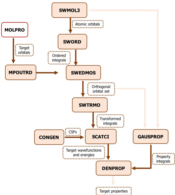
2.2 Flowchart for the target calculation using the UKRmol suite. The light beige filled boxes represent the programs called during the calculation; the boxes with the dashed brown border correspond to the data that are output from one program and serve as input to the following ones or are final results; the box with a red border corresponds to the programs that is not part of the UKRmol suite. . . 35 2.3 Flowchart for the inner region calculation using the UKRmol suite. The light beige
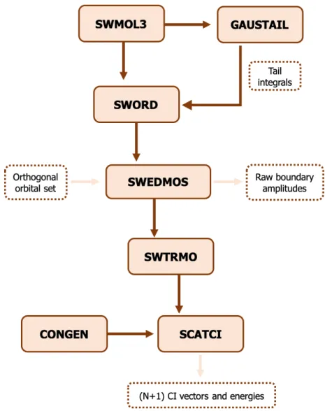
filled boxes represent the programs called during the calculation; the boxes with the dashed brown border correspond to the data that are output from one program and serve as input to the following ones or are final results. The "target orbitals"come from the target calculation, and the "raw boundary amplitudes"and "(N+1) CI vec-tors and energies"will be used as input in the outer region. . . 36 2.4 Flowchart for the outer region calculation using the UKRmol suite. The light beige
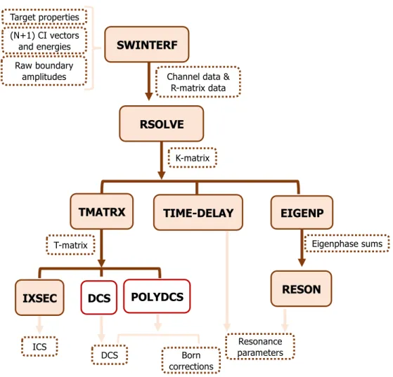
filled boxes represent the programs called during the calculation; the boxes with the dashed brown border correspond to the data that are output from one program and serve as input to the following ones or are final results; the boxes with a red border corresponds to the programs that is not part of the UKRmol suite. . . 37 2.5 Flowchart for the target calculation within the UKRmol+ suite. The light beige filled
boxes represent the programs called during the calculation; the boxes with the dashed brown border correspond to the data that are output from one program and serve as input to the following ones or are final results; the box with a red border corresponds to the programs that is not part of the UKRmol+ suite. . . 38 3.1 Chemical structure of para-benzoquinone. . . . 41 3.2 General chemical structure of ubiquinones (left) and pyrroloquinoline (right). . . . 42 3.3 Charge densities of the eight most diffuse orbitals calculated at HF and CASSCF
levels, using the cc-pVDZ basis set. The black dashed line represents the threshold of 1x10°6. . . . 49
3.4 Cross sections as a function of electron energy. Both curves were obtained with the same parameters at SE level (cc-pVDZ basis set, 10 VOs, deletion threshold of 10°7 and a = 13a0). The dashed blue curve corresponds to the inclusion of partial waves
up to lmax= 4, whereas the solid black line correspond to lmax= 5. . . 50
3.5 Cross sections as a function of electron energy calculated at SEP level, using the same parameters (cc-pVDZ basis set, deletion threshold of 10°7and a = 13a0), except for
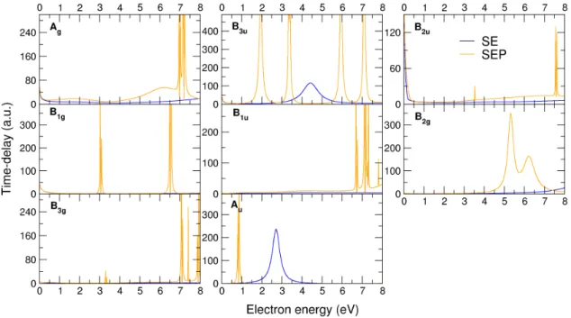
the number of VOs that is indicated the figure . . . 51 3.6 Largest eigenvalues of the time-delay matrix for the scattering symmetries indicated
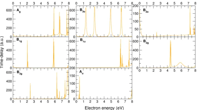
in the panels, at SE (solid blue line) and SEP (solid orange line) levels. . . 52 3.7 Largest eigenvalue of the time-delay matrix for the scattering symmetries indicated
in the panels, calculated at CC level. Note that most sharp peaks (that normally appear in more than one symmetry) correspond to excitation thresholds. . . 53
LI S T O FFI G U R E S
3.8 Cross sections as a function of electron energy, calculated at SEP and CC level, using the parameters described in table 3.3, for each of the irreducible representations indicated in the panels. The total cross section is shown in the right bottom panel. Note the y-axis is scaled for the elastic cross sections on the left, whereas the green labels on the right side of the plots correspond to the inelastic cross sections. . . 54 3.9 Inelastic cross sections as a function of electron energy, calculated at CC level, for
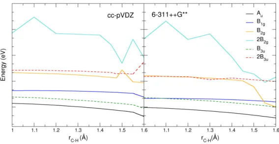
the irreducible representations presented in the panels. The energy grid used was of 0.002 eV. . . 59 3.10 Resonance energy as a function of C-H distance (in angstroms) for two basis sets,
calculated at SEP level. The C-H bond length in the equilibrium geometry is 1.095 Å. Please note the y-axis is not to scale: as the variation of the resonance positions with
rC °H is very small, we shifted some curves down to provide a better overview. The curve corresponding to the Auresonance remained unaltered; the remaining curves
were shifted down as follows: B3u1 eV, B1g 2 eV, B2g 3 eV, 2B3u 2 eV and 2B2g 3 eV.
For simplicity, and because the 1B2gand 3B3ubehaved completely non-dissociative
(as the 1Au, 1B3u, 1B1gand 2B3udo) we decided to omit their respective curves. . . 62
3.11 Eigenvalues of the time-delay matrix for the scattering symmetries indicated in the panels calculated at SEP level for the anion geometry. . . 65 3.12 Eigenvalues of the time-delay matrix for the scattering symmetries indicated in the
panels calculated at CC level for the anion geometry. Note that most sharp peaks (and the truncated ones) correspond to thresholds. . . 66 3.13 Resonance positions (in eV) for the neutral (left side) and anion geometry (right
side), calculated at CC level. Also presented are the vertical detachment energy (VDE), the vertical electron attachment (VEA) and the adiabatic electron attachment (AEA), estimated by us. The coloured horizontal lines correspond to resonances, with the energies for the anion geometry in the y-axis. . . . 68 3.14 Contributions to the integral elastic cross section from the scattering symmetries
indicated in the panels for the anion (dashed lines, black at CC and blue at SEP level) and neutral equilibrium geometries (solid lines, black at CC and green at SEP level): N.G. stands for neutral geometry and A.G. for anion geometry. The bottom right hand panel shows the total elastic cross sections(sum of all contributions shown in the other panels). . . 71 3.15 Contributions to the total integral inelastic cross section from the scattering
symme-tries indicated in the panels for the anion (light blue line) and neutral equilibrium geometries (black line). The bottom right hand panel shows the total integral inelas-tic cross sections (sum of all contributions shown in the other panels). . . 72 3.16 Differential cross sections as a function of electron energy, calculated at SEP and CC
levels. Also presented are the IAM-SCAR and the SMC results from Lozano et al. [101]. 73 4.1 Chemical structure of thiophene. . . 75
4.2 Chemical structure of tiaprofenic acid (1) and tenidap (2), two thiophene based non-steroidal anti-inflammatory drugs [124]. . . 76 4.3 Cross sections as a function of electron energy for two SE calculations using the same
parameters (6-311G** basis set, deletion threshold of 10°7and a = 15a0), and the
partial waves indicated. The dashed blue line correspond to the inclusion of partial waves up to lmax= 4, whereas the solid black line correspond to lmax= 5. Both were
calculated using the UKRmol suite. . . 83 4.4 Cross section as a function of electron energy, calculated at SEP level using the same
parameters (6-311G** basis set, deletion threshold of 10°7and a = 15a0), and the
number of VOs indicated in the figure. . . 84 4.5 Integral elastic cross section for electron scattering from thiophene for energies up to
10 eV calculated with the R-matrix approach at SEP and CC levels, with and without the Born correction (labeled Born in the former case). Also plotted are the SEP results from da Costa et al.[126]. . . . 85 4.6 Integral electronically inelastic cross section for electron scattering from thiophene
calculated using the R-matrix and IAM-SCAR methods [48]. R-matrix cross sections from calculations including partial waves up to lmax= 4 and lmax= 5 are plotted. . 86
4.7 Elastic differential cross sections for electron scattering from thiophene for the ener-gies indicated in the panels. The R-matrix DCS are Born corrected (labeled "Born"). The SMC-PP were calculated at SEP level and incorporate a Born based correc-tion [126]. . . 87 4.8 Calculated (full black lines) and measured (full orange line) excitation functions for
the energy losses indicated in the panels: left panels, scattering angle of 90±; right
panels scattering angle of 135±. The peaks of the measured excitation functions are
also indicated in the panels. The ¢E correspond to the energy losses measured by Regeta [47] and T1, T2 and S1 indicate the first and second triplet states, and the first singlet state, respectively. . . 88 4.9 Calculated and measured (full orange line) excitation functions for ¢E=5.41 eV
en-ergy loss, for the two angles indicated in the panels. The calculated curves corre-spond to increasing the number of states that are added. The labels on the right side of the panels indicate which states these are; T3corresponds to the third triplet state
(recall table 4.4), T4to the fourth, and so on. . . 89
4.10 The largest eigenvalue of the Q-matrix (time-delay) as a function of electron energy for the four irreducible representations that constitute the C2vpoint group. The
cal-culations were performed at SEP level with UKRmol suite, using a deletion threshold of 10°7, lmax= 5, the 6-311G** basis set and a = 15a0. . . . 91
4.11 Cross sections as a function of electron energy, calculated at SE (full black line) and SEP (full blue line) level, using the parameters listed in table 4.5 for the irreducible representations indicated in the panels. The total cross section is shown in the bottom panel. . . 92
LI S T O FFI G U R E S
4.12 The largest eigenvalue of the Q-matrix (time-delay) as a function of electron energy for the four irreducible representations of the C2v point group. The calculations
were performed at CC level with the UKRmol suite, using a deletion threshold of 10°7, lmax= 5, the 6-311G** basis set and a = 15a0. . . . 95
4.13 Cross sections as a function of electron energy, calculated at CC level using the pa-rameters listed in table 4.5. The full black line corresponds to the elastic cross section and the full orange line corresponds to the inelastic one. The total cross section is shown in the bottom panel. Note that the left side y-axis scale (in black) corresponds to the elastic cross section, whereas the right side one (in orange) corresponds to the inelastic cross section. . . 96 5.1 Chemical structure of conformer I of alanine. Note the stereochemistry. . . 101 5.2 Elastic cross section as a function of electron energy for two SE calculations using the
same parameters (6-311++G** basis set, deletion threshold of 10°17and a = 18a0),
but a different number of partial waves. Both were calculated using the UKRmol+ suite. The dashed blue line correspond to the inclusion of partial waves up to lmax=
4, whereas the solid black line correspond to lmax= 5. . . 108
5.3 The largest eigenvalue of the Q-matrix (time-delay) as a function of electron energy. The calculations were performed at SEP level, using a deletion threshold of 10°13,
10°14and 10°17. All calculations used 40 VOs, lmax= 5, the 6-311++G** basis set and
a = 18a0. . . 109
5.4 Cross sections as a function of electron energy. Both curves were obtained with the same parameters at SE level (the 6-311++G** basis set, 10 VOs, a deletion threshold of 10°17, lmax= 5 and a = 18a0). The full black curve was obtained using UKRmol+
suite, whereas the dashed blue curve was obtained using UKRmol. . . 110 5.5 The largest eigenvalue of the Q-matrix (time-delay) as a function of electron energy.
The calculations were performed at SEP level with UKRmol+ suite, using a dele-tion threshold of 10°17, lmax = 5, the 6-311++G** basis set, a = 18a0and the VOs
indicated in the figure. . . 111 5.6 Cross sections as a function of electron energy, for calculations at SEP level. The
full light blue line represents Fujimoto’s et al. [186] results obtained with UKRmol, and using the 6-311+G* basis set, a = 10a30, lmax = 4, a deletion threshold of 10°7
and 30 VOs; the dashed light blue line represents our attempt to reproduce Fuji-moto’s results, using his parameters and the UKRmol suite; finally, the solid green line represents the results using our parameters and UKRmol+. . . 112 5.7 Chemical structure of conformers II-B (left) and III-A (right) described by Császár [163],
and used by Fujimoto et al. [186]. . . 113 5.8 Cross sections as a function of electron energy for the conformers described by
Császár [163] as II-B and III-A. The full lines represent SEP calculations using the scattering parameters described by Fujimoto et al. [186], whereas the dashed lines used ours. . . 114
5.9 The largest eigenvalue of the Q-matrix (time-delay) as a function of electron energy. The full green line correspond to our SEP calculation using 40 VOs and the full purple line correspond to the SE calculation using 10 VOs. The number of VOs is the only parameter that is different between these two calculations. . . 115 5.10 The largest eigenvalue of the Q-matrix (time-delay) as a function of electron energy,
at CC level using 70 VOs. The narrow spikes correspond to excitation thresholds. . . 117 5.11 Cross sections as a function of electron energy, calculated at CC level. In the upper
panel, the orange full line represents elastic cross sections, and the dashed black line the inelastic cross sections. The total cross section is shown in the lower panel. Note that the scale for the inelastic cross section in the upper panel is indicated on the right side. . . 118 5.12 Inelastic cross sections as a function of electron energy calculated at CC level for
the number of VOs indicated in the figure. The remaining parameters are listed in table 5.4. . . 119 6.1 Flowchart for the inner region calculation using the UKRmol suite. The light beige
filled boxes represent the programs called during the calculation; the boxes with the dashed brown border correspond to the data that are output from one program and serve as input to the following ones or are final results; the ellipsis represent all the programs that run before and after swedmos, and that were already presented in chapter 2, figure 2.3. . . 128 6.2 Photodetachment spectrum of p-BQ°. The sharp features (labelled with F
corre-spond to features linked to Feshbach resonances, whereas the broad resonance (S) is of shape character. Taken from [83]. Please see reference for more information on the experimental procedure. . . 130 6.3 Photodetachment cross sections (in a20) as a function of the photon energy (in eV). 131 6.4 Action spectra for p-BQ°and p-BQ°-H2O depletion and H2O-loss from the complex.
The symbols correspond to raw data and the lines are 3-point moving averages. The dashed vertical lines correspond to the resonance positions obtained from Schiedt
et al. [83] from their photodetachment studies. The pictures were taken directly from
Stockett and Nielsen’s paper [50]. . . 133 6.5 Chemical structure of the p-BQ-H2O complex used in out calculations: the hydroxyl
group from the water is in the same plane as the p-BQ ring, whereas the other hy-drogen is perpendicular to that plane. . . 134 6.6 Cross sections as a function of electron energy for SE calculations using the same
parameters (cc-pVDZ basis set, deletion threshold of 10°7 and a = 16a0), and the
partial waves indicated for isolated p-BQ in the cluster geometry. The dashed blue line correspond to the inclusion of partial waves up to lmax= 4, the solid black line
corresponds to lmax = 5, and the dashed red line corresponds to lmax = 6. All of
LI S T O FFI G U R E S
6.7 Cross section as a function of electron energy, calculated at SE level using the pa-rameters listed in table 6.5. The dashed red line corresponds to the calculation performed using the ground state equilibrium geometry of p-BQ; the dotted blue line to the isolated p-BQ in the geometry it acquires in the complex; and the solid blue line to p-BQ-H2O in its ground state equilibrium geometry. . . 137
6.8 The largest eigenvalue of the Q-matrix (time-delay) as a function of electron energy, calculated at SE level, with the parameters listed in table 6.5. The dashed red line corresponds to the calculation performed using the ground state equilibrium geom-etry of p-BQ; the dotted blue line to the isolated p-BQ in the geomgeom-etry it acquires in the complex; and the solid blue line to p-BQ-H2O in its ground state equilibrium
geometry. . . 137 6.9 Cross section as a function of electron energy, calculated at SE level using the
pa-rameters listed in table 6.5. The dashed red line corresponds to the calculation performed using the anion ground state equilibrium geometry of p-BQ; the dotted black line to the isolated p-BQ in the geometry it acquires in the anion complex; and the solid black line to to p-BQ-H2O°in its ground state equilibrium geometry. . . . 139
6.10 The largest eigenvalue of the Q-matrix (time-delay) as a function of electron energy, calculated at SE level, with the parameters listed in table 6.5. The dashed red line corresponds to the calculation performed using the anion ground state (gs) equilib-rium geometry of p-BQ; the dotted black line to the isolated p-BQ in the geometry it acquires in the anion complex; and the solid black line to p-BQ-H2O°in its ground
state equilibrium geometry. . . 140 6.11 Cross section as a function of electron energy, calculated at SE level using the
pa-rameters listed in table 6.5 for the complex. The solid blue line corresponds to the calculation performed using the neutral equilibrium geometry of the complex, and the solid black line to the calculation using its anion equilibrium geometry. . . 142 6.12 The largest eigenvalue of the Q-matrix (time-delay) as a function of electron energy,
calculated at SE level, with the parameters listed in table 6.5. The solid blue line corresponds to the calculation performed using the neutral equilibrium geometry of the complex and the solid black line to the calculation using its anion equilibrium geometry. . . 142
L
I S T O F
T
A B L E S
3.1 Vertical excitation energies (in eV) obtained from CASSCF calculations using differ-ent states in the state-averaging procedure and differdiffer-ent active spaces for the three basis sets tested. Also presented are the experimental data from Koyanagi et al. [86, 87], Hollas et al. [109] and Horst et al. [89]. A.S. stands for Active Space; B.S. stands for basis sets; Conf. is the highest number of configurations generated per sym-metry, in this case the Ag; S.A. corresponds to the set of states averaged, and are
represented the letters X, Y and Z, where X: [1,1,0,1,2,0,2,1]; Y: [1,1,0,1,1,0,1,1]; and Z: [2,1,0,1,2,0,1,1]. The order of the symmetries is: ag, b3u, b2u, b1g, b1u, b2g, b3g
and au. Note that all the states averaged are singlets. E is the absolute energy of the
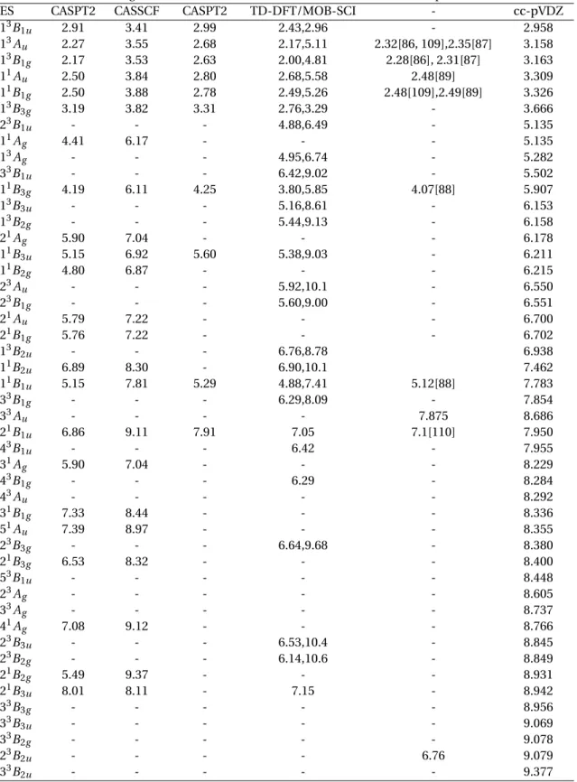
ground state (in Hartree) obtained at SA-CASSCF level. . . 47 3.2 Vertical excitation thresholds (in eV) obtained in this work from CASSCF
calcula-tions for the compact basis set, and the chosen active space and state-averaging. ES stands for Excited State. Also listed are the theoretical results obtained by Pou-Amérigo et al.[90] using CASPT2 and CASSCF methods; Scheiber et al. also using CASPT2 [92] and Jones et al. using TD-DFT and MOB-SCI/5s5p2d methods [93, 94]. The experimental values were obtained by Koyanagiet al. [86, 87], Hollas et al. [109], Trommsdorff [88], Horst et al. [89] and Jones et al. [94]. . . . 48 3.3 Parameters used for the SE, SEP and CC calculations presented in the remainder of
the chapter. . . 50 3.4 Positions and widths (in brackets) in eV of the low-lying resonances of p-BQ
calcu-lated at SEP and CC levels. Sym: below the former, the symmetry of the resonance ; C: Character. The capital letters mean: S: shape; M: mixed and F: Feshbach. We also list theoretical (Cheng et al.[104], West et al.[105], Kunitsa and Bravaya [107], Pou-Amérigo et al.[102], Honda et al.[103]) and experimental (Cooper et al.[91], Modelli and Burrow[99] and Allan[97, 98]) data available. The character of the resonances in the corresponding paper is indicated in brackets. . . 55
3.5 Positions and widths (in eV), and character of the resonances found in our CC calcu-lations as well as their most likely parent state(s) (P.S.). The capital letters mean: M: mixed shape core-excited; CE: core-excited shape. Earlier theoretical data: Cheng
et al. [104] (most results quoted are those from their non-averaged calculation; for
the 12B2gand 22B2g resonances we also quote the positions and widths from their
table 3. Also shown are their identified parent states.) and data from West et al. [105]. Experimental position of first2B2gresonance: Modelli and Burrow [99] and Allan [98]. 58
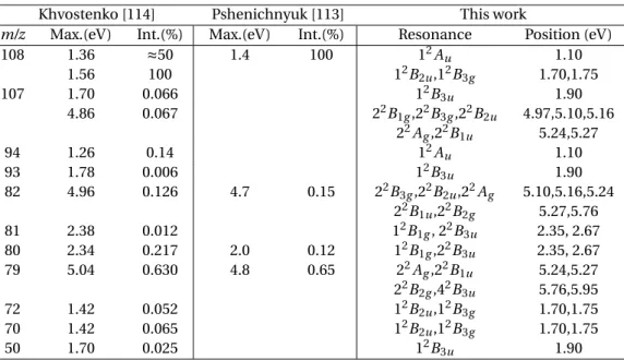
3.6 DEA peaks and respective m/z ratios and intensities from Pshenichnyuk et al. [113] and Khvostenko et al. [114], together with the resonances in our calculations most likely to lead to each of the DEA peaks, calculated at CC level. . . 61 3.7 Bond lengths (in Å) of p-BQ and p-BQ°in their respective equilibrium geometries. 64 3.8 Vertical excitation thresholds obtained in this work from CASSCF calculations. The
active space ((12,10)) and state-averaging (8 states: 11Ag, 11B3u, 11B1g, 1 ° 21B1u,
1 ° 21B3g and 11Au) were the same for both geometries, and was described before.
ES stands for Excited State, whose energies are presented in eV. . . 64 3.9 Positions and widths (in brackets, below the former), both in eV, of the six low-lying
resonances of p-BQ, calculated using its neutral (1A
g) and anion (2B2g) geometries,
at SEP and CC levels. The results presented for the neutral geometry were already shown (table 3.4) and discussed in the previous section. "Sym."indicates the symme-try of the resonance; and "Char."the respective character. The capital letters mean: S: shape; M: mixed shape core-excited and F: Feshbach. We also list theoretical work of: Kunitsa and Bravaya [107], Horke et al. [112], West et al. [105], Honda et al. [103] and Pou-Amérigo et al. [102]. The resonance positions presented by these authors were calculated using the ground state anion geometry. . . 67 3.10 VDE and AEA (both in eV) for the p-BQ anion. Also presented are the calculated
val-ues from Kunitsa and Bravaya [107], Horke et al. [112], Honda et al. [103] (computed at CASPT2 level) and Pou-Amérigo et al. [102]. . . . 69 3.11 Positions and widths (in eV), and character of the resonances found in our CC
cal-culations for the neutral and anion equilibrium geometries of p-BQ. The capital letters mean: M, mixed shape core-excited; CE, core-excited shape. The resonances labelled withT are only visible in the time-delay and therefore had their width de-termined by fitting those curves with the Breit-Wigner formula. The remaining reso-nances were fitted by an automated procedure in the RESON program (see chapter 2, section 2.6.1), that fits the eigenphase sums. . . 70 4.2 Character of the orbitals involved in the set of tested active spaces. . . 79 4.3 Energies (E, in Hartree) and dipole moment (µ, in Debye) of the ground state of
thiophene in its equilibrium geometry, obtained at HF and CASSCF levels, for each of the tested basis sets. Our CAS model used an active space of (10,9). The absolute state energies in brackets were calculated at HF level, using the same basis sets [108]; the dipole moment value in the last row was obtained experimentally [128]. . . 80
LI S T O F TA B L E S
4.4 Calculated vertical excitation thresholds (in eV) of the electronic states included in our CC calculations. Also listed are previous results from calculations: Salzmann
et al. [143], Kleinschmidt et al. [142], Holland et al. [145], Nakatsuji et al. [141],
Palmer et al. [131] (who also presents some EELs results) and Merchán et al. [138] (both CASSCF and PT2 results are presented); and experiments: Jones et al. [135], Regeta [47], Lonardo et al. [136], Flicker et al. [134], van Veen et al. [140], Asmis [132], Haberkern et al. [133] and Nyulászi et al. [137]. The energies labelled with a R cor-respond to Rydberg states. The vertical dots indicate that several other states are present in that energy range, for the calculation listed in that column. . . 81 4.5 Parameters used in the SE, SEP and CC calculations. . . 83 4.6 Positions and widths (in brackets) in eV of the low-lying shape resonances in
thio-phene taken from our time-delay analysis. The SEP results were calculated for 35 and 41 VO, whereas the CC calculation used 70 VOs. We list the calculated results from da Costa et al.[126] obtained using the SCM-PP method, Vinodkumar et al. [148] (R-matrix method) and the VAE obtained by Regeta [47] through the scaled Koopman’s theorem; the experimental resonance positions were obtained by Asmis [132] and Modelli and Burrow [146]. . . 92 4.7 Positions and widths in brackets (in eV) of the higher energy resonances in
thio-phene. Also listed are the experimental positions from the EELs measurements presented in section 4.4.3, and those obtained by Asmis [132]. These results are presented in ranges, determined from the positions of the peaks in the excitation functions for two angles (see figure 4.8). CE stands for pure core-excited resonances, MCES for mixed core-excited shape resonances and gs for ground state. The most likely parent states (PS) have been obtained from the branching ratios (when possi-ble). . . 97 4.8 DEA peaks [127] (or energy range where peaks were identified) and corresponding
resonances identified in our calculations. Please note that above a certain energy, it is impossible for us to confidently link a DEA peak with a specific resonance and therefore, we assigned them to any of the resonances in the corresponding energy range. . . 98
4.1 Vertical excitation energies (in eV) for the eight low-lying excited states of thiophene obtained including different states in the state-averaging procedure and using dif-ferent active spaces, for the diffuse basis set. Also listed are the respective ground state energies and dipole moments. A.S. stands for Active Space; Conf. corresponds to the number of configurations generated for the A1symmetry; and S.A. indicates
the choice of states we averaged. X: [2A1,3B2,1B1,1A2], Y: [2A1,1B2,0B1,0A2] and Z:
[2A1,2B2,1B1,1A2]. Note that all the states averaged are singlets. As the state
averag-ing Y provided the biggest disagreement with the experiments for the higher energy excitation thresholds, we did not test it with any other active spaces. The numbers in bold are the ones for the SA-CASSCF model we chose as the best set to perform our calculations. The ground states energies labelled6°311G§§andcc°pV DZ were calculated at MP2 level using the respective basis sets [108]. . . 100 5.1 Energies (E, in Hartree) and dipole moment (µ, in Debye) of the ground state of
ala-nine in its equilibrium geometry, obtained at HF and CASSCF levels, for each of the tested basis sets. Our CAS model used an active space of (8,6). Also presented are the more accurate results of Császár [163] (using 6-311++G**MP2/cc-pVTZ RHF model) for the ground state energy and the experimental dipole moment from Godfrey et
al. [166]. The calculation with the smallest basis set, 6-31G*, was performed in order
to replicate Fujimoto’s results [186], and therefore was performed only at HF level. . 105 5.2 Vertical excitation energies (in eV) obtained using different states in the state-averaging
procedure and different active spaces, for the 6-311++G** basis set. Also presented are ground state energy from Császár [163] and dipole moment obtained by Godfrey
et al. [166]. The experimental excitation energies obtained by Abouaf [161] are also
presented. A.S. stands for Active Space; Conf. corresponds to the number of config-urations generated and S.A. represents the number of states we averaged. Note that all the states averaged are singlets. . . 105 5.3 Vertical excitation energies, in eV, for the electronic excited states of alanine used
in our scattering calculations. The second, third and fourth columns correspond to our SA-CASSCF calculations using the active space (8,6) and several basis set. Also presented are the results of Osted et al. [178] calculated using the CCSD/aD(T) model and Kumar et al. [179] using the CIS/6-31G model. The experimental results were obtained by Abouaf [161]. The states labelled withRpossess Rydberg character. 106
5.4 Parameters used for the SE, SEP and CC calculations presented in the remainder of the chapter. . . 109 5.5 Parameters used by Fujimoto et al. [186]. No information was given regarding the
deletion threshold, so we assumed 10°7was used. The group also used the geometry
LI S T O F TA B L E S
5.6 Resonance positions (in eV) for alanine conformers (’Conf.’) I, II-B and III-A calcu-lated at SEP level: the time-delay analysis was used to locate the fist two resonances while the position of the third resonance was estimated from the cross section. The values marked withF were obtained by us using the parameters of Fujimoto’s et
al. [185]. The dipole moment (in Debye), µ, of the conformers determined in the
R-matrix calculations is listed in the last column. . . 113 5.7 Position and widths (in brackets), in eV, of the shape resonances identified in our
SE/SEP/CC calculations, as well as theoretical and experimental results from liter-ature. The results from Ptasi´nska et al. [188] and Scheer et al. [189] were obtained in DEA experiments, so the values correspond to peaks in the ion yield; Aflatooni
et al.’s [181] results come from ETS experiments; and Vasil’evet al. [190] recorded
resonant electron capture mass spectra. . . 116 5.8 Resonance positions (in eV) and widths (in eV, in brackets) for all resonances
iden-tified using the time-delay and cross sections analysis, from our SEP and CC cal-culations. "Ch"stands for character, "S": shape; "M": mixed shape-core-excited; "CE": core-excited. Also presented are the theoretical results obtained by Panosetti
et al. [184]; the R-matrix SEP results of Fujimoto et al. [186] and the SMC results of
Nunes et al. [187]. As for the experiments, the ETS results of Aflatooni et al. [181], some of the DEA results obtained by Ptasi´nska et al. [188] and Scheer et al. [189], and the Vasil’ev et al. [190] results obtained via resonant electron capture are also listed. 120 6.1 States, and respective energies (in H, with respect to the ground state 11Ag), included
in the photodetachment calculation and described as single excitations from the ground state configuration. Also presented are the energy of the states obtained in a more accurate calculation (see chapter 3). . . 128 6.2 Scattering parameters used in the photodetachment calculation. . . 129 6.3 Position and widths (in eV) and lifetimes (in ps, except the last one) of the
autode-taching states as observed in the photodetachment spectrum (see figure 6.2, taken from reference [83]). . . 129 6.4 Bond lengths (in Å) for the p-BQ-H2O cluster in the ground state equilibrium
geom-etry, as optimised by Stockett and Nielsen [50]. Also presented are the bond-lengths of the equilibrium geometry of the neutral (calculated at MP2/cc-pVDZ level [108]) and anion (optimised by Kunitsa and Bravaya [107] and used in our calculations in chapter 3) ground state of p-BQ. . . 134 6.5 Parameters used in our SE calculations. . . 135
6.6 Absolute energies (in Hatree) and dipole moment (µ) of the ground state of the com-plex p-BQ-H2O (in neutral and anion geometries) and isolated p-BQ. NC stands for
the geometry p-BQ possesses in the neutral complex; AC stands for its geometry in the anion complex; NG corresponds to the equilibrium ground state geometry of the neutral target; and AG to the equilibrium ground state geometry of the an-ion target. The energies in brackets were calculated by Stockett and Nielsen [50] at B3LYP/6-311++G* level. . . 136 6.7 Orbitals involved in the three resonances identified in the SE cross sections and
time-delay analysis for the neutral complex and isolated p-BQ (in the equilibrium ground state geometry). Resonance number 1 corresponds to electron attachment to the LUMO+1 orbital; number 2 to the LUMO+3 and number 3 to LUMO+5. NC means we are using the isolated p-BQ in the geometry it acquires in the neutral complex. . . 138 6.8 Positions and widths (in brackets) in eV for the resonances calculated at SE level
for the complex p-BQ-H2O and for the isolated p-BQ in the equilibrium ground
state and in the complex geometries. The labels are the following: NC stands for the geometry p-BQ possesses in the neutral complex;AC stands for its geometry in
the anion complex;NG corresponds to the equilibrium ground state geometry of the neutral target; andAG to the equilibrium ground state geometry of the anion target. The widths were obtained with RESON (see chapter 2), except the ones that are approximated values (preceded by º): those were obtained by a manual fit of the time-delay. . . 143 6.9 Shifts (in eV) in resonance positions of isolated p-BQ in the complex geometry, with
respect to isolated p-BQ in its ground state equilibrium geometry, for both neutral and anion geometries. . . 144 6.10 Shifts (in eV) in resonance positions of the complex, with respect to isolated p-BQ in
the complex geometry, for both neutral and anion geometries. . . 144 6.11 Shifts in resonance positions of isolated p-BQ in its equilibrium geometries with
respect to the complex in its equilibrium geometries. . . 144 6.12 Resonance positions (in eV) calculated for the equilibrium geometries of p-BQ°
and p-BQ-H2O°. ¢E corresponds to the energy difference between the resonance
A
C R O N Y M S
CAS Complete Active Space. CC Close-Coupling approximation. CE Core-excited resonance.
CSF Configuration state function. DCS Differential Cross Section. DEA Dissoactive Electron Attachment. DSB Double strand breaks.
EEL Electron Energy Loss. ES Excited state.
ETS Electron Transmission Spectroscopy. GS Ground state.
HF Hartree-Fock approximation.
HOMO Highest occupied molecular orbital. ICS Integral Cross Section.
LEE Low energy electrons.
LUMO Lowest unoccupied molecular orbital.
SA-CASSCF State-Averaged Complete Active Space Self Consistent Field approximation. SE Static Exchange approximation.
SEP Static Exchange plus Polarization approximation. SSB Single strand breaks.
VE Vertical excitation. VO Virtual orbital.
C
HAP
TER
1
I
N T R O D U C T I O N
One of the biggest challenges of this century is to respond to the medical needs of a growing and ageing population. Every day we assist to the appearance of more resistant diseases, in addition to several types of cancer that continue to affect a significant part of the world population (in 2017, 8.8 millions of people died from cancer [1]). The improvement and development of new treatments is therefore a major scientific concern. Highly energetic, ionising radiation (or primary radiation) has been applied in cancer treatment (radiotherapy) to around 50% of cancer patients [2]. Besides the direct effect of the primary radiation in human tissue, there are other processes involved, caused by the secondary species that are formed as a consequence of this first interaction. These processes cannot be disregarded, as we shall explain in this chapter.
Biological radiation damage (see figure 1.1 for an overview of the whole process) has been a very popular topic over the last decades, mainly from the physical-chemical perspective. The origin of this radiation can be natural or man made: a constant background of low intensity (but high energy) radiation is present all over the Earth, and comes essentially from cosmic radiation and due to the presence of radioactive Radon (222Rn) in the air, itself a product of the decay of radioactive uranium isotopes. With the rapid decrease of the ozone concentration in the stratosphere over the last decades, there has been an increased human exposure to ultravi-olet background (UVB) radiation. The energy quanta of UVB radiation (3.9-4.4 eV), although non-ionising, is capable of inducing molecular changes when interacting with biomolecular systems [3], as we will explain later on.
Besides the natural sources, human exposure to radiation can also occur for medical rea-sons: radiotherapy or medical imaging. Radiotherapy, as mentioned previously, is used to treat several types of cancer and it is relatively low cost compared to other treatments. Therefore, it is the more suitable procedure to use in developing countries, where cancer-survival rates are still very discouraging. Medical imaging consists mainly of tests that allow medical professionals to
Figure 1.1: Chronological diagram of radiation induced damage, adapted from [6]. "see inside the body"in order to diagnose, treat, and monitor health conditions. Medical imag-ing procedures are often used as a tool to determine the best treatment options for patients. The type of imaging procedure used depends on the health concern and the part of the body that is being examined. Some common examples of imaging tests include X-rays, computed tomography (CT), fluoroscopy and positron emission tomography (PET) [4, 5].
Over the last decades, there has been a lot of experimental and theoretical (see reference [7] and references therein, mainly in part I) work on quantification of the interaction of primary and secondary radiation with cell components and respective molecules. The radiation can be electromagnetic, electrons, positrons, protons, Æ-particles, neutrons and heavy charged ions. However, electrons (called secondary) are the major product of the interaction between ionizing radiation and a surrounding medium: around 104electrons with energies below 30
eV are generated per MeV of deposited radiation [8, 9]. As expected, and motivated by the pioneering work from Boudaïffa et al. from Leon Sanche’s group [10], the interaction between biomolecules and secondary electrons started receiving the attention of several groups all over the world [11, 12, 13, 14] (for a review see reference [3]). The experiments of Boudaïffa et al. were focused on DNA, and proved that electrons below the ionization threshold can produce single and double-strand breaks (SSBs and DBSs, respectively), through the Dissoactive Electron Attachment (DEA) process.
It is important to keep in mind that apart from DNA, cells contain a huge number of other important molecules, for example proteins and water, that are also potential targets for the incoming radiation, as we explain in the next section.
1.1 Radiation damage in biological systems
As mentioned earlier, when high-energy radiation interacts (or collides) with living tissue, it pro-duces a range of structural and chemical modifications that can affect biological function. These modifications can occur directly (when the primary radiation particle ionizes the molecules
1 . 2 . E L E C T R O N - M O L E C U L E C O L L I S I O N S directly, initiating a chain of events that leads to structural changes) or indirectly, through the production of intermediate species (free radicals and other particles like electrons, protons, etc.) that will damage the molecules. Our focus here is low energy electrons (LEEs, or secondary, as called before), the most abundant species produced during this interaction. The LEEs are generated by ionization processes, or formed by intermolecular Coulombic decay, which is a kind of non-local autoionization process [15]. They can also be formed by water radiolysis (dis-sociation of water molecules by ionizing radiation). Independent of their source, these LEEs can drive severe damage to biomolecules, which may lead to mutagenic, genotoxic and other lesions, in the case of DNA. After their production, these electrons gradually lose their kinetic energy through a series of inelastic interactions with the surroundings, until they reach near-zero energy, where we say they have been thermalised, or become solvated by the surrounding water [16].
The aim of studying LEEs collisions with biologically relevant molecules is to understand the mechanism of electron induced damage in these systems, and produce quantitative data to be used in modelling the radiation effects. Although the majority of the work has been performed in the gas phase (or as isolated molecules, in the case of computational studies), the reality is not that simple - in the cell, the target molecules are embedded in a specific environment that will affect the electron-molecule interaction and its outcome. The surroundings are mainly composed by water molecules, which triggered studies in pure and hydrated clusters [17, 18, 19]; studies in the condensed phase have also been performed (e.g. references [20, 21]).
There are plenty of other biologically relevant target molecules besides the extensively stud-ied nucleobases: sugars, aminoacids and smaller molecules that could serve as a model for more complex systems - e.g. proteins, that due to their size are impossible to model at the levels of accuracy required in our calculations. Therefore, the strategy used by theoreticians is to study the target’s central moiety, or smaller molecules that are similar enough, keeping the calculations within the computational limits. We will present some illustrative examples of this approach in section 1.5.
Beyond the importance of studying the interaction between LEEs and biological targets, electrons also play a crucial role outside the human context. Processes like photosynthesis, where electron transfer reactions have the most crucial role, are also attention worthy. Therefore, understanding the effects of electron collisions with the molecules that participate in these kind of processes is not only important, but needed. Para-benzoquinone (see chapter 3), (the prototypical member of the quinone’s family) is known to be involved in photosynthesis and respiration [22], and is one of the targets we studied during this thesis.
1.2 Electron-molecule collisions
As we have been discussing, a collision between an electron and a molecule can have serious implications on molecular structure and functioning. In this section we will present a brief overview of the electron-molecule collision process and its applications.
Electron-molecule collisions have been studied extensively by both experimentalists and theoreticians, especially over the last two decades. This was stimulated by mainly two factors: (i) the emergence of more powerful computers that allow the study of more complex targets and more collision processes more accurately; and (ii) the increasing development of experimental instrumentation (improved electron spectrometers, intense sources of spin-polarised electrons, position-sensitive detectors, etc.) [23].
Electrons, particularly, play a central role in atomic and molecular physics, as their small mass makes them much more mobile than the nuclei. The understanding of their behaviour is essential to understand a large variety of problems in many areas of physics (such as gas lasers, laboratory plasmas, ionospheres, auroras, stellar atmospheres, interstellar gases and more recently, and more relevant to this thesis, radiation induced damage) whose advance is dependent on the availability of data on collision processes between electrons, ions, and neutral atoms and molecules. The subject of atomic and molecular collisions is itself of great intrinsic interest, having played a leading role in the establishment of quantum theory [23].
Electron-molecule collisions are significantly more difficult to study than electron-atom collisions, due to the following reasons:
• Molecules have rotational and vibrational degrees of freedom. Those can be excited by a much smaller amount of energy than electronic excitations. As a result, rotational and vibrational excitations are the dominant energy-loss processes below the electronic excitation threshold of the target molecule;
• The electron-molecule short-range interaction is essentially multi-centred and non-spherical because molecules are characterised by the presence of more than one nucleus. Even at large separations, the interaction is often strong and orientation dependent since molecules have various permanent electric multipole moments. Furthermore, the polaris-ability of the target molecule, which determines the polarisation force is also anisotropic; • Molecular targets can dissociate in collision with an electron, as we will explain later on. 1.2.1 Low-energy electron processes
In section 1.1, we expressed our interest in electron-molecule collisions with electrons de-fined as "low-energy", as their energy lay below the ioniastion threshold of the target molecule (around 10-15 eV). In this energy range, any of the following processes can happen [24] (the processes are listed in approximate order of increasing kinetic energy of the projectile):
• Elastic scattering: where the internal state of the target and the kinetic energy of the incoming electron are not affected.
AB + e°! AB + e°
• Rotational excitation: the rotational state of the target (denoted by j ) is changed, as well as the energy of the incoming electron.
1 . 3 . R E S O N A N C E S ABj+ e°! ABj0+ e°
• Vibrational excitation: the vibrational state of the target (denoted by v) is changed, as well as the energy of the incoming electron.
ABv+ e°! ABv0+ e°
• Electronic excitation: the electronic state of the target (denoted by i ) is changed, as well as the energy of the incoming electron.
ABi+ e°! ABi0+ e°
• Electron impact dissociation: the target is excited into a dissoactive state, leading to its neutral fragmentation. The formation of the intermediate AB§°(also known by temporary
negative ion, TNI°, or resonance) is not necessary.
AB + e°! [AB§°] ! A + B + e°
• Dissoactive electron attachment (DEA): the incoming electron is trapped in a resonant state, cleaves one molecular bond (or more) and remains attached to one of the fragments, whereas the other (or others) are neutral.
AB + e°! AB§°! A + B°+ e°(or A°+ B + e°)
The DEA process is responsible for molecular bonds cleavage in biological targets, as ex-plained (although the electron impact dissociation also leads to molecular break-up). The first step of the whole process is the formation of a resonance (AB§°). To fully comprehend the DEA mechanism, it is crucial to understand the behaviour and the characteristics of resonances, as they determine the fate of the target molecule. The DEA process will be discussed in more detail later on this chapter.
1.3 Resonances
Resonances are electronic states embedded in a continuum (except vibrational Feshbach res-onances - VFRs, as we will explain later) and, as a consequence, are always susceptible to spontaneous electron loss (autodetachment). Although electron loss can happen very quickly, a potential energy barrier prevents the electron from leaving instantly [25]. An atom or a molecule can have many different electronic resonances, but each of those can only occur for a particular energy of the incoming electron. By definition, a resonance has a negative electron affinity and is characterized by its energy E and width °, where the latter is related to its half-time (or lifetime) ø, through the expression below:
Resonances can be observed in a number of calculated and/or measured scattering quan-tities. For example, they manifest themselves as peaks in the integral cross section for elastic and inelastic scattering and as sudden changes of approximately º in the eigenphase sum (see chapter 2). They are also visible as peaks in the time-delay (also defined in chapter 2).
Resonances can be classified according to whether they involve fundamentally the tronic states of the target or they involve nuclear (vibrational) degrees of freedom. The elec-tronic resonances can be classified as:
• Shape resonances: The electron attaches to the target molecule in its ground electronic state (that is then described as the parent state of the resonance), usually at low incident electron energies (approximately up to the energy of the first excited threshold of the target - above this energy most resonances usually have core-excited character). These resonances are seen as trapping of the incoming electron in one of the unoccupied or-bitals of the target molecule - they are 1 particle 0 hole states. The potential energy curve of a shape resonance lies above the one of the neutral molecule. However when this resonance has energy close to the ground state energy, the potential energy curve may be below the ground state energy for some geometries and the resonant state becomes bound [26]. The lifetime differs between molecules and between resonances in the same molecule, and can be of the order of ten femtoseconds to milliseconds. Because they tend to be relatively close in energy to the ground state, these resonances are usually short-lived.
• Core-excited resonances: The resonance is formed when the incoming electron elec-tronically excites the target molecule to an excited state (the parent state), and at the same time, it is temporarily trapped in one of the unoccupied orbitals. The description of the core-excited resonances usually involves single excitations of the target molecule, i.e. they are 2 particle 1 hole states. These resonances usually occur at higher incident electron energies than shape resonances (since some energy is needed to excite the tar-get first). We can divide core-excited resonances into two different types: Feshbach and core-excited-shape resonances [27].
1. Feshbach resonances: These resonances lie energetically below the parent state and are typically weakly bound. They tend to have much longer lifetimes than both shape and core-excited shape resonances, and therefore are very narrow which makes them very hard to detect experimentally, due to the experimental instrumen-tation resolution. This is because the autodetachment channel to the parent state is closed i.e., the decay to the parent state is energetically forbidden, and consequently, its decay occurs into some nonparent state(s).
2. Core-excited shape resonances: The approaching electron has enough energy to elec-tronically excite the molecule to which the electron is concurrently trapped. These resonances lie above the parent state into which they can decay through the au-todetachment process that is usually short. The name itself implies similarities to
1 . 3 . R E S O N A N C E S the shape resonances, as their mechanism of formation is the same except that the attractive part of effective potential arises between the incoming electron and the target molecule in an electronically excited state.
Other type of Feshbach resonances are VFRs: they involve nuclear motion and usually occur at very low energies when the electron is trapped into a diffuse (dipole-bound) state and its energy is transferred to the molecular vibrations. VFRs are likely to occur in molecules with large polarizabilities and/or a very large dipole moment, and can be found just below the thresholds for vibrational excitation of the target molecule.
Figure 1.2 summarizes the types of resonances we just described, their usual lifetimes and where their relative positions are with respect to electronic states of the target.
Figure 1.2: Schematic figure of the relative position of shape, core-excited shape and Feshbach resonances and respective usual lifetimes. The size of the grey boxes is not representing their width. AB stands for a generic target molecule. The horizontal lines in the energy axis corre-spond to the ground state (AB) and an excited state (AB§) energies.
In our calculations we have identified several resonances that we characterize as of mixed character. These resonances do not have a shape or core-excited character, but are, in fact, a mix of both. They possess more than one parent state (state the electron attaches to in the scattering process), one of them the ground state, and the remaining an electronically excited state(s).
As metastable states, resonances can decay very easily (unless they become bound, as men-tioned previously). This decay depends on several factors as: the lifetime of the resonances, if the resonance formed is dissoactive, how fast the nuclei moves, how far from the equilibrium geometry the anion becomes bound, etc.; we can have mainly two types of decay, schematized in figure 1.3:
• Autodetachment (AD)
It is the most probable channel leading to decay of a shape resonance, where the autode-tached electron has the same energy as the incoming electron. In the case of core-excited
Figure 1.3: Possible pathways for a resonance decay. After its formation, electron loss through autodetachment can occur or DEA into fragments, one of them negatively charged.
resonances, some part of the initial kinetic energy of the electron can be left within the molecule (i.e. to use in the rotational, vibrational, electronic degrees of freedom excita-tion).
• Dissociative electron attachment (DEA)
It is the most likely decaying channel for resonances with a long lifetime. The dissociation process is bond selective, that is, the bonds that break in a molecule are dependent on the incident electron energy, as shown in the work of Denifl et al. [14] and many others. Multiple bond cleavages and new bond formation are also possible as a result of DEA. Figure 1.4 (adapted from [28]) illustrates the potential energy diagram for the DEA process of a diatomic molecule.
This process requires a bit more of our attention as it is one of the main reasons why we are interested in identifying and characterizing resonances. As the anionic product can be detected straight after molecule cleavage by conventional mass spectrometry, DEA has become very popular and extensive studies have been performed. The kinetic energy of the fragments is determined by the asymptotic behavior of the potential energy curves and the internal energies of the products. DEA dynamics involves a strong interaction between the electron motion and nuclear motion, and this makes its the theoretical description particularly challenging [29].
Despite its importance in electron-induced fragmentation of biomolecules, DEA has also important applications in industry (like FEBID [30] - Focused Electron Beam Induced Deposi-tion - and industrial plasmas) as well as occurring naturally, for example, in the Earth ionosphere where oxygen radical anions are formed by DEA from molecular oxygen.
However, dissociation and autodetachment are not the only possible fates of a resonance. As we will present and discuss in chapter 3, there are molecules (as p-BQ) capable of accept and retain electrons. This means that their resonances are fairly stable, and their energy is
1 . 3 . R E S O N A N C E S
Figure 1.4: Scheme of the DEA process for a diatomic molecule AB, representing the poten-tial energy Epotential as a function of the bond length (r). The A-B and [A-B]° curves are the
potential energy of the neutral and anion molecules, respectively. Eincidentis the energy of the
incident electron; Ebindingthe energy needed to dissociate the bond. The dashed horizontal
line represents the vibrational energy. For r > rC, the anion becomes bound, and stable against
autoionization. Therefore, if the molecule reaches this point before autoionizing, DEA will occur.
dissipated through the nuclear degrees of freedom of the molecule, until it reaches the bound anionic state, that is more stable than the neutral ground state.
1.3.1 Cross sections
One of the main ways of quantifying the effect of a collision is by measuring (or calculating) a cross section: they can be defined as a measure of probability that a specific process will take place in a collision of two targets.
Cross sections can be classified in several ways: as an integrated quantity over all param-eters, and therefore called integral cross sections (or ICS); or as differential cross sections (DCS), when it is specified as a function of some final-state variable, in our case the scattering angle. The former depends only on the scattering energy, whereas the latter can be presented as angular DCS - provided for a specific scattering energy as a function of the scattering angle; or what we usually call excitation functions - provided for a specific scattering angle as a function of scattering energy.
Cross sections can either be determined for a specific process or for a sum of these, re-ferred to as total cross sections (TCS), that quantify the probability that all scattering processes take place and are easily measured. Elastic cross sections (ECS) quantify the probability of the