High-precision measurements of
n
=
2
→
n
=
1 transition energies and level
widths in He- and Be-like argon ions
J. Machado,1,2C. I. Szabo,3,4J. P. Santos,1,*P. Amaro,1M. Guerra,1A. Gumberidze,5Guojie Bian,2,6 J. M. Isac,2and P. Indelicato2,†
1Laboratório de Instrumentação, Engenharia Biomédica e Física da Radiação (LIBPhys-UNL), Departamento de Física,
Faculdade de Ciências e Tecnologia, FCT, Universidade Nova de Lisboa, P-2829-516 Caparica, Portugal
2Laboratoire Kastler Brossel, Sorbonne Université, CNRS, ENS-PSL Research University, Collège de France, Case 74; 4, Place Jussieu,
F-75005 Paris, France
3
National Institute of Standards and Technology, Gaithersburg, Maryland 20899, USA
4Theiss Research, La Jolla, California 92037, USA
5ExtreMe Matter Institute EMMI and Research Division, GSI Helmholtzzentrum für Schwerionenforschung, D-64291 Darmstadt, Germany
6Institute of Atomic and Molecular Physics, Sichuan University, Chengdu 610065, People’s Republic of China
(Received 5 July 2017; published 26 March 2018)
We performed a reference-free measurement of the transition energies of the 1s2p1P
1→1s2 1S0 line in He-like argon, and of the 1s2s22p1P
1→1s22s2 1S0 line in Be-like argon ions. The highly charged ions were produced in the plasma of an electron-cyclotron resonance ion source. Both energy measurements were performed with an accuracy better than 3 parts in 106, using a double flat-crystal spectrometer, without reference to any theoretical or experimental energy. The 1s2s22p1P
1→1s22s2 1S0 transition measurement is the first reference-free measurement for this core-excited transition. The 1s2p1P
1→1s2 1S0 transition measurement confirms recent measurement performed at the Heidelberg electron-beam ion trap. The width measurement in the He-like transition provides test of a purely radiative decay calculation. In the case of the Be-like argon transition, the width results from the sum of a radiative channel and three main Auger channels. We also performed multiconfiguration Dirac-Fock calculations of transition energies and rates and have done an extensive comparison with theory and other experimental data. For both measurements reported here, we find agreement with the most recent theoretical calculations within the combined theoretical and experimental uncertainties.
DOI:10.1103/PhysRevA.97.032517
I. INTRODUCTION
Bound-state quantum electrodynamics (BSQED) and the relativistic many-body problem have been undergoing im-portant progress in the past few years. Yet there are several issues that require increasing the number of high-precision tests. High-precision measurements of transition energies on medium to high-Z elements [1–9], Landégfactors [10–16], and hyperfine structure [17–29], just to name a few, are needed either to improve our understanding or to provide tests of higher-order quantum electrodynamics (QED) corrections, the calculations of which are very demanding.
Recent measurement of the proton size in muonic hydrogen [30,31] and of the deuteron in muonic deuterium [32], which disagree by 7 and 3.5 standard deviations, respectively, from measurements in their electronic counterparts triggered experimental and theoretical research regarding not only the specific issue of the proton and deuteron size, but also the possible anomalies in BSQED. A discrepancy of this magnitude corresponds to a difference in the muonic hydrogen energy of 0.42 meV, which is far outside the calculation uncertainty of about±0.01 meV and is much larger than what
can be expected from any omitted QED contribution. Another large discrepancy of 7 standard deviations between theory and experiment has also been observed recently in a specific difference between the hyperfine structures of hydrogenlike and lithiumlike bismuth measured at the experimental storage ring (ESR) at GSI in Darmstadt [29], designed to eliminate the effect of the nuclear magnetization distribution (the Bohr-Weisskopf correction) [22].
Medium and high-Z few-electron ions with aK hole are the object of the present work. They have been studied first in laser-produced plasmas [33] and beam-foil spectroscopy (see, e.g., [34,35]), low-inductance vacuum spark [36], or by using the interaction of fast ion beams with gas targets in heavy-ion accelerators. Ion storage rings have also been used (see, e.g., [37–39]). The limitation in precision of those measurements is mostly due to the large Doppler effect, which affects energy measurements, and the Doppler broadening, which affects any possible width measurement.
Recoil ion spectroscopy [40], which has also been used, is not affected by the Doppler effect, and provides an interesting check. Plasma machines, such as tokamaks, have also provided spectra [41,42], leading to relative measurements, without Doppler shift, usually using He-like lines as a reference. Solar measurements [43] have also been reported.
an electron beam ion trap (EBIT) or electron-cyclotron ion sources (ECRISs) to produce ions at rest in the laboratory. Such measurements, using an EBIT, have been performed by the Livermore group (see, e.g., [8,44–47] and references therein), the Heidelberg group [1,4,9,48], and the Melbourne and National Institute of Standards and Technology (NIST) collaboration [3,5,6]. The present collaboration has reported values using an ECRIS [2].
The Heidelberg group reported the measurement of the 1s2p1P1→1s2 1S0He-like argon line with a relative accuracy
of 1.5×10⁻⁶without the use of a reference line [48]. In that
work, the spectrometer used is made of a single flat Bragg crys-tal coupled to a charge-coupled device (CCD) camera, which can be positioned very accurately with a laser beam reflected by the same crystal as the x rays [48]. The Melbourne-NIST collaboration reported the measurement of all the n=2→
n=1 transitions in He-like titanium with a relative accuracy of 15×10−6, using a calibration based on neutral x-ray lines
emitted from an electron fluorescence x-ray source [3,5,6]. The Livermore group reported a measurement of alln=2→
n=1 lines in heliumlike copper [8], using hydrogenlike lines in argon as calibration. It also reported measurement of all four lines in He-like xenon, using a microcalorimeter and calibration with x-ray standards [49]. It should be emphasized that measurements in both types of ion sources do not require Doppler shift correction to transition energy measurements, because the ions have only thermal motion.
Measurements of the 1s2s22p1P1→1s22s2 1S0 line in
Be-like ions are scarce. Some measurements are relative measurements using tokamaks, where the Be-like line ap-pears as a satellite line for the He-like 2→1 transitions. The 1s2p1P1→1s2 1S0 line is often used as a calibration.
Measurements of that type for Be-like Ar have been performed at the Tokamak de Fontenay aux Roses (TFR) [50], and for Ni at the Tokamak Fusion Test Reactor (TFTR) [41,42]. Such relative measurements, which use theoretical results on the He-like line, must be recalibrated using the most recent theoretical values. Several other observations have been made on different elements, but no experimental energy reported (see, e.g., Ref. [51] for Cl, Ar, and Ca), or the experimental accuracy is not completely documented (see, e.g., [52–54]). Measurements in EBIT are also known, as in vanadium [55] and iron [56], for terrestrial and astrophysics plasma applications. There have also been relative measurements in ECRIS for sulfur, chlorine, and argon [57], using the relativistic M1 transition 1s2s3S
1→1s2 1S0as a reference.
Chantleret al.[3,5,58], have claimed that existing data show the evidence of a discrepancy between the most advanced BSQED calculation [59] and measurements in the He-like isoelectronic sequence, leading to a deviation that scales as ≈Z3. They speculated [5] that this supposed systematic effect
could provide insight into theproton size puzzle, the Rydberg and fine-structure constants, or missing three-body BSQED terms. Here we make a detailed analysis, including all available experimental results, to check this claim.
We emphasize the advantage of studying highly charged, medium-Z systems, such as argon ions, to test QED. The BSQED contributions have a strongZdependence: The retar-dation correction to the electron-electron interaction contribu-tion scales asZ3, and the one-electron corrections, self-energy
and vacuum polarization, scale asZ4. Yet, at highZ, the strong enhancement of the nuclear size contribution and associated uncertainty limits the degree to which available experimental measurements can be used to test QED [58,60–63]. At very low Z, experiments can be much more accurate, but tests of QED can be limited as well, even for very accurate measurements of transitions to the ground state of He [64–66]. For few-electron atoms and ions, they are limited by the large size of electron-electron correlation and by the evaluation of the needed higher-order QED screening corrections, in the nonrelativistic QED formalism (NRQED) [67–71]. It can also be limited by the slow convergence of all-order QED contributions at low Z, which may be required for comparison, and because of the insufficient knowledge of some nuclear parameters, namely the form factors and polarizability [30–32,59]. In medium-Z elements like argon or iron, the nuclear mean spherical radii are sufficiently well known (see, e.g., [72]) and nuclear polarization contribution to the ion level energies is very small. So uncertainties related to the nucleus are small compared to experimental and theoretical accuracy. This can be seen in the theoretical uncertainties claimed in Ref. [59].
Besides the fundamental aspect, knowledge of transition energies and wavelengths of highly charged ions is very important for many sectors of research, such as astrophysics or plasma physics. For example, an unidentified line was recently detected in the energy range 3.55–3.57(3) keV in an x-ray multimirror (XMM-Newton) space x-ray telescope spectrum of 73 galaxy clusters [73] and at 3.52(3) keV for another XMM spectrum in the Andromeda galaxy and the Perseus galaxy cluster [74]. The next year a line at 3.53(11) keV was observed in the deep exposure data set of the Galactic Center region with the same instrument. A possible connection with a dark matter decay line has been put forward, yet measurements performed with an EBIT seem to show that it could be a set of lines in highly charged sulfur ions, induced by charge exchange [75], while a recently published search with the high-resolution x-ray spectrometer of the HITOMI satellite does not find evidence for such lines in the Perseus cluster [76]. In the present work, we apply the method we have devel-oped to measure the energy and linewidth of the 1s2s3S
1→
1s2 1S0 M1 transition reported in Ref. [2], to the 1s2p1P1→
1s2 1S0 transition in He-like argon and to the 1s22s2p1P1→
1s22s2 1S0 transition in Be-like argon ions. We also present
a multiconfiguration Dirac-Fock (MCDF) calculation for the two transition energies and widths. These calculations are performed with a new version of theMCDFGMEcode that uses the effective operators developed by the St. Petersburg group to evaluate the self-energy screening [77].
The article is organized as follows. In the next section we briefly describe the experimental setup used in this work. A detailed description of the analysis method that provides the energy, width, and uncertainties is given in Sec. III. A brief description of the calculations of transition energy and widths is given in Sec.IV. We present our experimental result for the 1s2p1P
1 →1s2 1S0 transition in Sec. V. In the same
section we present all available experimental results for 7
the 1s2s22p1P1→1s22s2 1S0 line in Be-like argon ions are
presented in Sec.VI. The conclusions are provided in Sec.VII.
II. EXPERIMENTAL METHOD
ECRIS plasmas have been shown to be very intense sources of x rays, and have diameters of a few centimeters. Therefore, they are better adapted to spectrometers that can use an extended source. At low energies one can thus use cylindrically or spherically bent crystal spectrometers as well as double-crystal spectrometers (DCSs).
A single flat-crystal spectrometer, combined with an accu-rate positioning of the detector, and alternate measurements, symmetrical with respect to the optical axis of the instrument, as used in Heidelberg [48], and the double-crystal spectrom-eters [78,79] are the only two methods that can provide high-accuracy, reference-free measurements in the x-ray domain. We use here reference free with the same meaning as in Ref. [80], i.e., the measured wavelengths are directly connected to the meter as defined in the International System of Units, through the lattice spacing of the crystals [79]. Our group reported in 2012 such a measurement of the 1s2s3S1 →1s2 1S0
transition energy in He-like argon with an uncertainty of 2.5×10⁻⁶without the use of an external reference [2], using
the same experimental device as in the present work: a DCS connected to an ECRIS, the “Source d’ Ions Multichargés de Paris” (SIMPA) [81], jointly operated by the Laboratoire Kastler Brossel and the Institute des Nanosciences de Paris on the Université Pierre and Marie Curie campus.
A detailed description of the experimental setup of the DCS at the SIMPA ECRIS used in this work is given in Ref. [79]. A neutral gas (Ar in the present study) is injected into the plasma chamber inside a magnetic system with minimum fields at the very center of the vacuum chamber. Microwaves at a frequency of 14.5 GHz heat the electrons that are trapped by the magnetic field. The energetic electrons ionize the gas through repeated collisions reaching up to heliumlike charge states [82]. The ions are, in turn, trapped by the space charge of the electrons, which have a density around 1×1011cm−3. This corresponds to a
trapping potential of a fraction of 1 V, leading to an ion-speed distribution of≈1 eV per charge, and thus to a small Doppler broadening of all the observed lines. In contrast, EBITs have a trapping potential of several hundred eV, and the Doppler broadening is then much larger.
The 1s2s3S
1state is mostly created by electron ionization of
the 1s22s2S
1/2ground state of Li-like argon, and therefore the
1s2s3S1→1s2 1S0 line is the most intense line we observed
in He-like argon. The 1s2p1P1→1s2 1S0 line observed here
results from the excitation of the 1s2 1S0He-like argon ground
state, which is much less abundant, leading to a weaker line. The Be-like excited level, 1s2s22p1P
1, is mostly produced
by ionization of the ground state of boronlike argon, which is a well-populated charge state (see Fig. 21, Ref. [79]). The 1s2s22p1P1→1s22s2 1S0 line is thus the most intense we
observed.
The spectra are recorded by a specially designed, reflection vacuum double-crystal spectrometer described in detail in Ref. [79]. The two (6×4) cm2, 6 mm-thick Si(111) crystals
were made at the National Institute for Standards and Technol-ogy (NIST). Their lattice spacing in vacuum was measured and
found to be d111=3.135601048(38) ˚A (relative uncertainty
of 0.012×10⁻⁶) at a temperature of 22.5◦C [79], relative
to the standard value [83,84]. More details will be found in Ref. [85]. Using this lattice spacing, our measurement provides wavelengths directly tied to the definition of the meter [84]. The DCS is connected to the ion source in such a way that the axis of the spectrometer is aligned with the ECRIS axis and is located at 1.2 m from the plasma (a sphere of≈3 cm in diameter).
To analyze the experimental spectra, we developed a simu-lation code [79], which uses the geometry of the instrument and of the x-ray source, the shape of the crystal reflectivity profile, as well as the natural Lorentzian shape of the atomic line and its Gaussian Doppler broadening to perform high-precision ray tracing. The reflectivity profile is calculated using the x-ray oriented program (XOP) [86], which uses dynamical diffraction theory from Ref. [87], and the result is checked with the X0H program, which calculates crystal susceptibilitiesχ0
andχh[88,89].
The first crystal is maintained at a fixed angle. A spectrum is obtained by a series of scans of the second crystal. A stepping motor, driven by a microstepper, runs continuously, between two predetermined angles that define the angular range of one spectrum. X rays are recorded continuously and stored in a histogram, together with both crystal temperatures. Succes-sive spectra are recorded in opposite directions. Both crystal angles are measured with Heidenhain1high-precision angular encoders. The experiment is performed in the following way: a nondispersive-mode (NDM) spectrum is recorded first. Then a dispersive-mode (DM) spectrum is recorded. The sequence is completed with the recording of a second NDM spectrum. Due to the low counting rate, such a sequence of three spectra takes a full day to record. In order to obtain enough statistics, the one-day sequence is repeated typically 7–15 times.
III. DATA ANALYSIS
The data analysis is performed in three steps. First we derive a value for the experimental natural width of the line. For this, each experimental dispersive-mode spectrum is fitted with simulated spectra, using an approximate energy (e.g., the theoretical value) and a set of Lorentzian widths. A weighted one-parameter fit is performed on all the results for all recorded dispersive-mode spectra providing a width value and its uncertainty. This experimental width is then used to generate a new set of simulations, using several different energies and crystal temperatures. These simulations are used to fit each dispersive-mode and nondispersive-mode experimental spectrum in order to obtain the line energy. For each day of data recording this leads to two Bragg angle values, obtained by taking the angular difference between a nondispersive-mode spectrum and a dispersive-mode spectrum.
(1) One Bragg angle value is obtained by comparing the first nondispersive-mode spectrum of the day and the dispersive-mode spectrum obtained immediately after.
(2) A second Bragg angle value is obtained by comparing the same dispersive-mode spectrum with the nondispersive-mode spectrum obtained immediately after.
In that way a number of possible time-dependent drifts in the experiment are compensated. We now describe these processes in more detail.
A. Evaluation of the widths
The ion temperature, which is necessary to calculate the Gaussian broadening was obtained by measuring first a line with a completely negligible natural width, the M1 1s2s3S1→1s2 1S0, transition. The width of this transition is ≈1×10⁻⁷eV, which is totally negligible when compared to
our spectrometer inherent energy resolution. From this analysis we obtained the Gaussian broadening ŴGExp.=80.5(46) meV [2]. This value also provides the depth of the trapping potential due to the electron space charge. Knowing the experimental Gaussian broadening value ŴExp.G , we can perform all the needed simulations. For each line under study we then proceed as follows.
(1) Perform simulations for the dispersive-mode spectra for a set of natural width values ŴiL and the theoretical transition energyE0, using the already knownŴExp.G , and crystal
temperatureTRef.= 22.5◦C.
(2) Interpolate each simulation result with a piecewise spline function to obtain a set of continuous, parametrized functions S[E
0,ŴLi,Ŵ Exp.
G ,T](θ−θ0), where θ0 correspond to the angle at which the simulation reaches its maximum value, and T =TRef..
(3) Normalize all the functions above to have the same maximum value (we chose the one withŴL=0 as reference).
(4) Fit each experimental spectrum with the functions obtained above,
I(θ−θ0,Imax,a,b)=ImaxS[E0,ŴiL,Ŵ Exp.
G ,T](θ−θ0)+a+bθ, (1)
whereImaxis the line intensity,θthe crystal angle,athe
back-ground intensity, andbthe background slope. The parameters θ0,Imax,a, andbare adjusted to minimize the reducedχ2(ŴLi).
We perform a series of fits of each experimental spectrum, with 27 simulated spectra, each evaluated with a different widthŴi
L,
to obtain a set of χ2(Ŵi
L) values. The width values go from
0 to 250 meV by steps of 10 meV, completed by a point at 300 meV. A typical experimental spectrum and the fitted simulated functions, for five of the 27 values of ŴLi used to make the analysis, are shown in Fig.1.
(5) Fit a third degree polynomial to the set of points [ŴLi,χ2(ŴLi)].
(6) Find the minimum of the third degree polynomial to get the corresponding optimalŴL opt.n ,nbeing the experiment run number (see Fig.2for an example).
(7) Get the 68% error barδŴn
L opt.for experiment runnby
finding the values of the width for which [90]
χ2ŴL opt.n ±δŴnL opt.=χ2ŴL opt.n +1. (2)
51.94 51.96 51.98 52 52.02 52.04 52.06 52.08 52.1 52.12 52.14
Angle (degrees) 1
1.5 2 2.5 3 3.5
counts/s
Experiment natural width = 0 meV natural width = 70 meV natural width = 150 meV natural width = 200 meV natural width = 300 meV
FIG. 1. Example of a dispersive-mode experimental spectrum for the He-like Ar 1s2p1P
1→1s2 1S0 transition (black dots), together with a few plots of the function in Eq. (1), for different values of the natural line widthŴi
L. The four parameters have been adjusted to minimize the reducedχ2(Ŵ
L) (see text for more explanations).
(8) Finally a weighted average of the values in the set of all theŴL opt.n obtained for all measured spectra is performed to obtain the experimental valueŴExp.L and its error bar:
1
δŴLExp.2
=
n
1
δŴn L opt.
2,
ŴLExp.=δŴLExp.2
n
Ŵn L opt.
δŴL opt.n 2
. (3)
The sets ofŴnL opt. for both lines studied here are plotted in Fig.3.
The two first steps are performed by two different methods, one based on the Centre Européen de Recherche Nucléaire (CERN) programROOT, version 6.08 [91–93], and one based onMATHEMATICA, version 11 [94].
Natural width (meV)
0 20 40 60 80 100 120 140 160
2
χ
115 120 125 130 135 140
FIG. 2. Third degree polynomial fitted to the [ŴL,χ2(ŴL)] set of points (black dots), for the He-like Ar 1s2p1P
1 2 3 4 5 6 7 measurement number
40 60 80 100 120 140
Width (meV)
Natural width Weighted average
σ +
σ
-1 2 3 4 5 6 7 8 9 10 11 12 13 14 measurement number
110 120 130 140 150 160 170 180 190
Width (meV)
Natural width
Weighted average
σ +
σ -(a)
(b)
FIG. 3. Natural width values of all the spectra recorded during the experiment, with weighted average and uncertainties evaluated with Eq. (3). (a) He-like argon 1s2p1P
1→1s2 1S0 transition. (b) Be-like argon 1s2s22p1P
1→1s22s2 1S0transition.
B. Transition energy values
Once we obtained the experimental width valueŴExp.L of a measured line (cf. Sec. III A), the determination of the correspondent experimental transition energy value Eexp is
achieved using the following scheme.
(1) Perform simulations in the nondispersive and disper-sive modes for a set of transition energy valuesEk=Etheo+
kE, whereEtheois the theoretical energy value,Ean energy
increment, andkan integer that can take positive or negative values. The simulations are done with the experimental natural widthŴLExp. and Gaussian broadeningŴGExp.. The simulations are performed at various crystal temperature valuesTlfor each
energy.
(2) As in Sec.III A, interpolate each simulation result with a spline function for both the nondispersive and dispersive modes, to obtain a set of functions depending on all the (Ek,Tl)
pairs.
(3) Fit each experimental spectrum, using Eq. (1) with E0=Ek andT =Tl, to obtain the angle difference between
the simulation and the experimental spectrum, both in disper-sive and nondisperdisper-sive modes.
Temperature (C)
18 19
20 21
22 23
24 25
26 27
Energy (eV)
3139.50 3139.55 3139.60 3139.65
Angle offset difference (Degrees)
0.004
−
0.003
−
0.002
−
0.001
−
0.000 0.001 0.002 0.003
FIG. 4. Fitted two-dimensional function from Eq. (4), and experi-mental results (white spheres), for the He-like Ar 1s2p1P
1→1s2 1S0 transition. The fit is performed taking into account the statistical error bars in each point.
(4) For each pair of dispersive- and nondispersive-mode experimental spectra, calculate the offsets θExp.n,k,l−Simul.= (θExp.DMn −θExp.NDMn )−(θSimul.DMk,l −θSimul.NDMk,l ) between the simulated spectra and the experimental value obtained in the step above. This offset should be 0 if the energy and tempera-ture used in the simulation were identical to the experimental values.
(5) Fit the bidimensional function,
θExp.-Simul.(E,T)=p+qE+rE2+sET+uT +vT2,
(4)
wherep,q,r,s,u, andvare adjustable parameters, to the set of points [Ek,Tl,θ
n,k,l
Exp.−Simul.] obtained in the previous step (see
Fig.4as an example).
(6) The experimental line energyEExp.n for spectrum pair numbern, is the energy such thatθExp.−Simul.(EExp.n ,TExp.)=0
whereTExp., stands for the average measured temperature on
the second crystal.
(7) As a check, we also used the line energy such that θExp.−Simul.(EnExp.,TRef.)=0 (TRef.=22.5◦C). This leads to a
temperature-dependent energy. We then fitted a straight line to the line energy, as a function of the second crystal temperature, and extrapolated toT =22.5◦C. Both methods lead to very
close values, well within the uncertainties.
(8) As in Sec.III A, we calculate the weighted average of all the (n,EExp.n ) pairs to obtain the final experimental energy. The error bar on each point is the quadratic combination of the instrumental uncertainty, as given in Table I, and of the statistical error.
(9) To check the result, we also fit the set of (EnExp.,TExp.n ) pairs with the function E0+bT to check that there is no
residual temperature dependence.
IV. THEORETICAL CALCULATION
The core-excited 1s2s22p1P1 →1s22s2 1S0 transition in
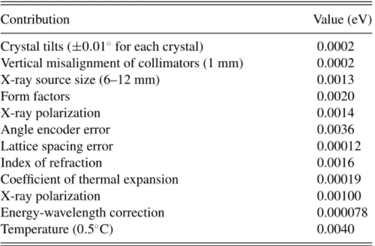
TABLE I. Instrumental contributions to the uncertainties in the analysis of the daily experiments (see Refs. [2,79]).
Contribution Value (eV)
Crystal tilts (±0.01◦for each crystal) 0.0002 Vertical misalignment of collimators (1 mm) 0.0002 X-ray source size (6–12 mm) 0.0013
Form factors 0.0020
X-ray polarization 0.0014
Angle encoder error 0.0036
Lattice spacing error 0.00012
Index of refraction 0.0016
Coefficient of thermal expansion 0.00019
X-ray polarization 0.00100
Energy-wavelength correction 0.000078
Temperature (0.5◦C) 0.0040
Previous calculations [97–100] did not take into account QED and relativistic effects to the extent possible today.
For the preparation of this experiment, we performed a cal-culation of the energy value for the 1s2s22p1P1→1s22s2 1S0
transition in Be-like argon, using the multiconfiguration Dirac-Fock approach as implemented in the 2017.2 version of the relativistic MCDF code (MCDFGME), developed by Desclaux and Indelicato [101–104]. The full description of the method and the code can be obtained from Refs. [101,105–107]. The present version also takes into account the normal and specific mass shifts, evaluated following the method of Shabaev [108–
110], as described in [111,112].
The main advantage of the MCDF approach is the ability to include a large amount of electronic correlation by taking into account a limited number of configurations [113–115]. All calculations were done for a finite nucleus using a uniformly charged sphere. The atomic masses and the nuclear radii were taken from the tables by Audi et al. [116] and Angeli and Marinova [72,117], respectively.
Radiative corrections are introduced from a full QED treatment. The one-electron self-energy is evaluated using the one-electron values of Mohr and co-workers [118–122], and corrected for finite nuclear size [123]. The self-energy screen-ing and vacuum polarization were included usscreen-ing the methods developed by Indelicato and co-workers [102,103,124–126].
In previous work, the self-energy screening in this code was based on the Welton approximation [102,103]. Here we also evaluate the self-energy screening following the model oper-ator approach recently developed by Shabaevet al.[77,127], which has been added toMCDFGME. A detailed description of
this new code will be given elsewhere.
In order to assess the quality of this new method for calcu-lating the self-energy screening we can compare the different values for the He-like transition measured here. The QED value of Indelicato and Mohr [128] is 0.1100 eV, and the one from Ref. [59] (TableIV) is 0.1085. The Welton method provides 0.0916 eV, while the implementation of the St. Petersburg effective operator method gives 0.0965 eV, closer to the ab initiomethods. We can thus assume an uncertainty of 0.014 eV and 0.018 eV for the effective operator and Welton operator methods, respectively. The same procedure applied to the Be-like transitions provides 0.130 eV using Ref. [128], 0.112 eV for the effective operator method and 0.109 eV for the Welton method. We can conclude that at intermediateZ, both the Wel-ton and effective operator methods provide very similar results, the effective operator method being in slightly better agreement withab initiocalculation. This is consistent with earlier com-parisons for fine-structure transitions (see, e.g., Ref. [129]).
Lifetime evaluations are done using the method described in Ref. [130]. The orbitals contributing to the wave function were fully relaxed, and the resulting nonorthogonality between initial and final wave functions fully taken into account, following [131,132].
The full Breit interaction and the Uehling potential are in-cluded in the self-consistent field process. Projection operators have been included [107] to avoid coupling with the negative energy continuum.
As a check, we also performed a calculation of the He-like argon lines measured in the present work and in Ref. [2]. Following Refs. [107,133–135], we use for the excited state the following configurations:
1s2p1P1=c1|1s2p,J =1 +c2|2s3p,J =1 +c3|2p′3d,J =1 +c4|3s4p,J =1 +c5|3p′4d,J =1 +c6|3d′4f,J =1 +c7|4s5p,J =1 +c8|4p′5d,J =1 +c9|4d′5f,J =1 +c10|4f′5g,J =1
TABLE II. Total energy and transition energies (in eV) for the 1s2s22p1P
1→1s22s2 1S0transition in Be-like argon, as a function of the maximum principal quantum numbernof the correlation orbitals. All correlation from the Coulomb, retardation, and QED parts is included. Extrapolation forn→ ∞is done by fitting the functiona+b/n2+c/n3to the correlation energy [difference with the energy fornand the Dirac-Fock (DF) value] of each level and retaining only the constant terma. The uncertainty combines the difference between the extrapolated and best directly calculated value, the missing Auger shift, and the self-energy screening model.
Welton QED Model operator QED [77,127]
n Initial Final Transition Initial Final Transition
DF −7222.7485 −10313.5817 3090.8333 −7222.7522 −10319.3215 3096.5692
2 −7227.3514 −10319.3250 3091.9736 −7227.3551 −10319.3320 3091.9769
3 −7228.6879 −10320.5341 3091.8462 −7228.6915 −10320.5417 3091.8502
4 −7229.0470 −10320.7556 3091.7086 −7229.0506 −10320.7638 3091.7131
5 −7229.1988 −10320.8783 3091.6795 −7229.2024 −10320.8870 3091.6846
TABLE III. Convergence of theoretical partial radiative widths, Auger widths, and energies for transitions originating from the Be-like 1s2s22p1P
1level. Transition energies are in eV and widths in meV.
Radiative Auger
→1s22s2 1S
0 →1s22s2S1/2 →1s22p2P1/2 →1s22p2P3/2
Max.n Energy Width Energy Width Energy Width Energy Width Total width
DF 3096.57 62.79 2240.96 0.52 2208.96 14.36 2205.80 48.87 126.54
2 3091.98 64.58 2237.06 24.34 2205.22 3.64 2201.85 8.83 101.39
3 3091.85 63.43 2236.33 1.29 2204.44 2.24 2201.23 6.30 73.26
4 3091.71 63.11 2236.12 0.22 2204.24 16.13 2201.06 49.29 128.75
5 3091.68 63.12 2235.99 0.29 2204.14 2.34 NC
+c11|5s6p,J =1 +c12
5p′6d,J =1
+c13|5d′6f,J =1 +c14|5f′6g,J =1 +c15|5g′6h,J =1, (5)
where thel′indicates an orbital with identical angular function
as thelone, but with another radial wave function, for which the orthogonality with orbitals of the same symmetry in another configuration is not enforced. The ground-state wave function is taken as usual as |1s2 1S0 =c1|1s2,
J =0 +c2|2s2,J =0 +c3|2p2,J =0 + · · · +c20|6g2,
J =0 +c21|6h2,J =0. We also evaluated
1s2s3S1=c1|1s2s,J =1 +c2|2p3p,J =1 +c3|3s4sJ =1 +c4|3d4d,J =1 +c5|4p5p,J =1 +c6|4f5f,J =1 +c7|5s6s,J =1 +c8|5d6d,J =1
+c9|5g6g,J =1, (6)
in order to calculate the M1 transition energies measured in Ref. [2], which allowed one to compare also energy differ-ences.
For Be-like argon, the correlation contributions result from the inclusion of all single, double, and triple electron ex-citations of the n=1 and 2 electrons in the unperturbed configuration up ton=5. For the 1s22s2 1S
0 ground state it
corresponds to 2478 configurations and for the 1s2s22p1P1
excited state to 14 929 configurations. We performed an estimation of the full correlation energy by doing a fit with the function a+b/n2+c/n3, and extrapolation ton→ ∞ for each level, for both the Welton and the Model operator values. The results are presented in TableII. By comparing the extrapolated value and the changes in QED due to the use of either the Welton or effective operator method we estimated the theoretical uncertainty provided in the table. There is, however, a contribution that is not included, the Auger shift. This shift is due to the fact that the 1s2s22p1P
1 being core excited is
degenerate with a continuum. To our knowledge, such shifts have been evaluated only in the case of neutral atom x-ray spectra [124,125,136]. For argon with a 1shole, the shift is 165 meV, while for a 2p hole it is 11 meV. Here we have a four-electron system, with only three possible Auger channels, and the 2sshell is closed, so the effect is expected to be small. We assume an extra theoretical uncertainty of 11 meV for this uncalculated term.
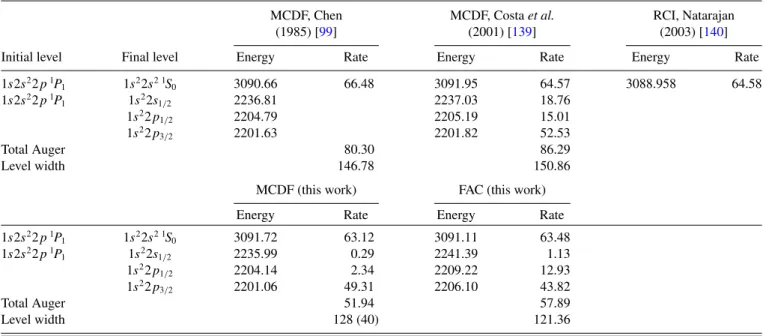
TABLE IV. Comparison between theoretical partial radiative widths, Auger widths, and energies for transitions originating from the Be-like 1s2s22p1P
1level. Transition energies are in eV and widths in meV.
MCDF, Chen MCDF, Costaet al. RCI, Natarajan (1985) [99] (2001) [139] (2003) [140]
Initial level Final level Energy Rate Energy Rate Energy Rate
1s2s22p1P
1 1s22s2 1S0 3090.66 66.48 3091.95 64.57 3088.958 64.58 1s2s22p1P
1 1s22s1/2 2236.81 2237.03 18.76
1s22p
1/2 2204.79 2205.19 15.01
1s22p
3/2 2201.63 2201.82 52.53
Total Auger 80.30 86.29
Level width 146.78 150.86
MCDF (this work) FAC (this work)
Energy Rate Energy Rate
1s2s22p1P
1 1s22s2 1S0 3091.72 63.12 3091.11 63.48 1s2s22p1P
1 1s22s1/2 2235.99 0.29 2241.39 1.13
1s22p
1/2 2204.14 2.34 2209.22 12.93
1s22p
3/2 2201.06 49.31 2206.10 43.82
Total Auger 51.94 57.89
TABLE V. Measured and computed natural line width values for the 1s2p1P1→1s2 1S0transitions in He-like Ar. All values are given in meV, and estimated uncertainties are shown in parentheses.
Transition Experiment Theory Reference
1s2p1P
1→1s2 1S0 75 (17) 70.4778 (25) MCDF (this work)
70.40 MBPT, Siet al.(2016) [145] 70.43 MCDHF, Siet al.(2016) [145] 70.43 Johnsonet al.(1995) [142] 70.49 (14) Drake (1979) [141]
The Auger width of the 1s2s22p1P
1 level is calculated
with theMCDFGME code, following the method described in Ref. [137] with full relaxation and final-state channel mixing, again taking into account the nonorthogonality between the initial and final state. For the first time, we combine this method with fully correlated wave functions, up ton=5. The convergence of the transition energy and width are presented in TableIII. This table shows that the Auger width values vary rather strongly when increasing the maximum n of correla-tion orbitals, when nonorthogonality and full relaxacorrela-tion are included. This behavior is due to the fact that the free electron wave functions have to be orthogonal to all the occupied and correlation orbitals of the same symmetry, which provides a lot of constraints.
We have also performed calculations of the transition energies and rates with the “flexible atomic code” (FAC), widely used in plasma physics [138]. This code is based on the relativistic configuration interaction (RCI), with independent
particle basis wave functions that are derived from a local cen-tral potential. This local potential is derived self-consistently to include the screening of the nuclear potential by the electrons. The final results are compared to other calculations from Refs. [99,139,140] in TableIV. The relatively large difference between our present MCDF calculation and the Dirac-Fock calculation from Ref. [139], made with an earlier version of our code, is due to correlation and to the evaluation of Auger rates using fully relaxed initial and final states.
The contributions of all the other possible transitions to the 1s2nl Jlevels,n=3→ ∞, were evaluated by computing all
Auger widths up to n=9,l=8. We then fitted a function a/n2+b/n3 to the total Auger width for each principal quantum numbern, summing all values ofLandJ for each value of n, to evaluate the contribution from n=10 up to infinity. We finda =0.056 2325 meV andb=0.530 28 meV. The total value for the contribution of all levels withn3 is 0.063 meV and is thus negligible.
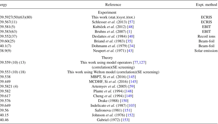
TABLE VI. Comparison of our He-like argon experimental 1s2p1P
1→1s2 1S0transition energy with previous experimental and theoretical values. All energies are given in eV, and estimated uncertainties are shown in parentheses.
Energy Reference Expt. method
Experiment
3139.5927(50)(63)(80) This work (stat.)(syst.)(tot.) ECRIS
3139.567(11) Schlesseret al.(2013) [57] ECRIS
3139.581(5) Kubičeket al.(2012) [48] EBIT
3139.583(63) Bruhnset al.(2007) [1] EBIT
3139.552(37) Deslatteset al.(1984) [40] Recoil ions
3139.60(25) Briandet al.(1983) [35] Beam-foil
3140.1(7) Dohmannet al.(1979) [34] Beam-foil
3138.9(9) Neupertet al.(1971) [43] Solar emission
Theory
3139.559 (10) (13) This work using model operators [77,127] (correlation)(SE screening)
3139.553 (10) (18) This work using Welton model (correlation)(SE screening)
3139.538 MBPT, Siet al.(2016) [145]
3139.449 MCDHF, Siet al.(2016) [145]
3139.5821 (4) Artemyevet al.(2005) [59]
3139.582 Planteet al.(1994) [148]
3139.617 Chenget al.(1994) [149]
3139.576 Drake (1988) [150]
3139.649 Indelicatoet al.(1987) [103]
3139.56 Safronova (1981) [151]
3140.15 Johnsonet al.(1976) [152]
1 2 3 4 5 6 7 8 9 10 11 12 13 14 measurement number
3139.580 3139.585 3139.590 3139.595 3139.600 3139.605
Energy (eV)
Transition energy Weighted average Statistical error
σ +
σ
-FIG. 5. He-like argon 1s2p1P
1→1s2 1S0transition energy val-ues of the different spectra recorded during the experiment. Error bars in each point correspond to the quadratic sum of the peak fitting uncertainty with the uncertainties from TableI, which have random fluctuations only, i.e., the angle measurement and the temperature correction. The (pink) shaded area corresponds to the weighted average of the peak position statistical uncertainty obtained from the fit. The±1σ lines combine these statistical uncertainties with all systematic errors from TableI. Every pair of points corresponds to one-day data taking (see text for explanations).
V. RESULTS AND COMPARISON WITH THEORY FOR THE HE-LIKE 1s2p1P1
→1s2s1S0TRANSITION
A. Line widths
Our experimental values for the line widths, obtained as explained in Sec.III Aand Fig.3(a), are presented in TableV, together with several theoretical results. There are several possible E1 radiative transitions originating from the 1s2p1P
1
level. Because of the large energy difference, the contribution of the 1s2p1P1→1s2 1S0 transition to the level width is
strongly dominant. The next largest contribution, due to the 1s2p1P
1→1s2s1S0transition, contributes only 0.0001 meV
to the 70.4-meV width. The width of the n=2→n=1 transitions has been calculated using Drake’s unified method [141], relativistic random phase approximation, MCDF, rela-tivistic configuration interaction (RCI) and QED [142]. The effect of the negative energy continuum has been discussed in Refs. [135,143]. Radiative corrections to the photon emission have also been evaluated [144]. The differences between all theoretical values and our measurement are well within the experimental error bar.
B. Transition energies
We present in Fig.5the transition energy values obtained from the successive pairs of dispersive and
nondispersive-TABLE VII. Summary of all measuredn=2→n=1 transition energies in He-like ions 7Z20. The theoretical values are from Ref. [59], which are available forZ12. The experimental values are either reference-free measurements (RF) or measurements calibrated against standard reference x-ray transitions, or hydrogenlike transitions (SR).
1s2p1P
1→1s2 1S0(w) 1s2p3P2→1s2 1S0(x) 1s2p3P1→1s2 1S0(y) 1s2s3S1→1s2 1S0(z)
Z Expt. (eV) Err. Theory Expt. (eV) Err. Theory Expt. (eV) Err. Theory Expt. (eV) Err. Theory Method Ref.
7 430.6870 0.0030 SR [155]
8 573.949 0.011 SR [155]
11 1126.72 0.31 SR [33]
12 1352.329 0.015 1352.2483 1343.5417 1343.0988 1331.1118 SR [33]
13 1598.46 0.31 1598.2914 1588.7611 1588.1254 1574.9799 SR [33]
14 1864.76 0.42 1865.0014 1854.6679 1853.7804 1839.4495 SR [33]
15 2152.84 0.56 2152.4310 2141.3188 2140.1082 2124.5619 SR [33]
16 2461.27 0.49 2460.6292 2448.7628 2447.1439 2430.3512 SR [33]
16 2460.69 0.15 2460.6292 2448.7628 2447.1439 2430.3512 SR [36]
16 2460.630 0.021 2460.6292 2448.7628 2447.1439 2430.3512 RF [7]
16 2460.670 0.090 2460.6292 2448.7628 2447.05 0.11 2447.1439 2430.3512 SR [156]
18 3139.5821 3126.2896 3123.5344 3104.1605 0.0077 3104.1483 RF [2]
18 3139.5821 3128 2 3126.2896 3123.5344 3104.1483 SR [157]
18 3139.5927 0.0076 3139.5821 3126.2896 3123.5344 3104.1483 RF This work
18 3139.5810 0.0092 3139.5821 3126.2896 3123.5344 3104.1483 RF [7]
18 3139.552 0.037 3139.5821 3126.283 0.036 3126.2896 3123.521 0.036 3123.5344 3104.1483 SR [40]
18 3139.57 0.25 3139.5821 3126.37 0.40 3126.2896 3123.57 0.24 3123.5344 3104.1483 SR [35]
19 3510.58 0.12 3510.4616 3496.4937 3492.9736 3472.2417 SR [158]
20 3902.43 0.18 3902.3777 3887.7607 3883.3169 3861.2059 SR [36]
20 3902.19 0.12 3902.3777 3887.63 0.12 3887.7607 3883.24 0.12 3883.3169 3861.11 0.12 3861.2059 SR [54]
21 4315.54 0.15 4315.4124 4300.1720 4294.6220 4271.0997 SR [158]
21 4315.35 0.15 4315.4124 4300.23 0.15 4300.1720 4294.57 0.15 4294.6220 4271.19 0.15 4271.0997 SR [53]
22 4749.73 0.17 4749.6441 4733.8008 4726.9373 4701.9746 SR [158]
22 4749.852 0.072 4749.6441 4733.83 0.13 4733.8008 4727.07 0.10 4726.9373 4702.078 0.072 4701.9746 SR [6]
23 5205.59 0.55 5205.1653 5188.7378 5180.3264 5153.8962 SR [36]
23 5205.26 0.21 5205.1653 5188.7378 5180.3264 5153.8962 SR [158]
TABLE VIII. Summary of all measuredn=2→n=1 transition energies in He-like ions 21Z92. The theoretical values are from Ref. [59]. The experimental values are either reference-free measurements (RF) or measurements calibrated against standard reference x-ray transitions, or hydrogenlike transitions (SR).
1s2p1P
1→1s2 1S0(w) 1s2p3P2→1s2 1S0(x) 1s2p3P1→1s2 1S0(y) 1s2s3S1→1s2 1S0(z)
Z Expt. (eV) Err. Theory Expt. (eV) Err. Theory Expt. (eV) Err. Theory Expt. (eV) Err. Theory Method Ref.
24 5682.66 0.52 5682.0684 5665.0715 5654.8491 5626.9276 SR [36]
24 5682.32 0.40 5682.0684 5665.0715 5654.8491 5626.9276 SR [158]
26 6700.76 0.36 6700.4347 6682.3339 6667.5786 6636.6126 SR [36]
26 6700.73 0.20 6700.4347 6682.3339 6667.5786 6636.6126 SR [158]
26 6700.441 0.049 6700.4347 6682.3339 6667.5786 6636.6126 RF [7]
26 6700.90 0.25 6700.4347 6682.50 0.25 6682.3339 6667.50 0.25 6667.5786 6636.6126 SR [160]
26 6700.549 0.070 6700.4347 6682.3339 6667.671 0.069 6667.5786 6636.6126 RF [4]
27 7245.88 0.64 7242.1133 7223.4718 7205.9299 7173.4164 SR [36]
28 7805.75 0.49 7805.6053 7786.4246 7765.7048 7731.6307 SR [36]
29 8391.03 0.40 8391.0349 8371.3181 8346.9929 8311.3467 SR [36]
29 8390.82 0.15 8391.0349 8371.17 0.15 8371.3181 8346.99 0.15 8346.9929 8310.83 0.15 8311.3467 SR [8]
30 8997.53 0.65 8998.5238 8978.2677 8949.8740 8912.6466 SR [36]
31 9627.45 0.75 9628.2072 9607.4099 9574.4461 9535.6292 SR [36]
32 10 280.70 0.22 10 280.2175 10 259.52 0.37 10 258.8739 10 221.79 0.35 10 220.7996 10 181.33 0.52 10 180.3868 SR [44]
36 13 115.45 0.30 13 114.4705 13 090.8657 13 026.8 3.0 13 026.1165 12 979.2656 SR [161]
36 13 114.68 0.36 13 114.4705 13 091.17 0.37 13 090.8657 13 026.29 0.36 13 026.1165 12 979.63 0.41 12 979.2656 SR [45]
36 13 114.47 0.14 13 114.4705 13 090.8657 13 026.15 0.14 13 026.1165 12 979.2656 RF [9]
38 14 666.8 6.1 14 669.5399 14 644.7518 14 562.2995 14 512.1996 SR [36]
39 15 475.6 2.9 15 482.1565 15 456.7619 15 364.1984 15 312.4664 SR [36]
54 30 629.1 3.5 30 630.0512 30 594.3635 30 209.6 3.5 30 206.2652 30 129.1420 SR [162]
54 30 619.9 4.0 30 630.0512 30 594.3635 30 210.5 4.5 30 206.2652 30 126.70 3.90 30 129.1420 SR [163] 54 30 631.2 1.2 30 630.0512 30 594.50 1.70 30 594.3635 30 207.1 1.4 30 206.2652 30 129.1420 SR [49]
59 37 003.7270 36 964.0900 36 389.1 6.8 36 391.2920 36 305.1570 SR [47]
92 100 626 35 100 610.89 100 537.18 96 169.63 96 027.15 SR [164]
92 100 598 107 100 610.89 100 537.18 96 169.63 96 027.15 SR [165]
mode spectra, recorded during the experiment for the He-like argon 1s2p1P1 →1s2 1S0 following the method presented in
Sec.III. The weighted average and±1σ bands are plotted as well.
TableVIpresents the measured He-like argon 1s2p1P1 →
1s2 1S0transition energy, together with all known
experimen-tal and theoretical results. The final experimenexperimen-tal accuracy, combining the instrumental contributions from Table I is
2.5×10⁻⁶. The value is in agreement with a preliminary
result, obtained with the same setup, but using fit with Voigt profiles of both the experimental spectra and the simulations [146,147]. The agreement with the most precise experiments, i.e., the two reference-free experiments [1,48] and the recoil ion experiment of Deslatteset al.[40] is well within combined error bars. The agreement with the calculation of Artemyev et al.[59] is also within the linearly combined error bars.
TABLE IX. Summary of alln=2→n=1 transition energies in He-like ionsZ7, calibrated relative to the theoretical value of one of the four He-like transitions (x, y, z, or w). The line used as calibration is noted “Ref.”. The energies of the measured lines have been re-evaluated using Ref. [59] for the reference transition energy. The displayed theoretical values are also from Ref. [59].
1s2p1P
1→1s2 1S0(w) 1s2p3P2→1s2 1S0(x) 1s2p3P1→1s2 1S0(y) 1s2s3S1→1s2 1S0(z)
Z Expt. (eV) Err. Theory Expt. (eV) Err. Theory Expt. (eV) Err. Theory Expt. (eV) Err. Theory Ref.
16 2460.6292 2448.739 0.020 2448.7628 2447.150 0.009 2447.1439 Ref. 2430.3512 [57] 18 3139.567 0.011 3139.5821 3126.291 0.011 3126.2896 3123.489 0.012 3123.5344 Ref. 3104.1483 [57] 18 Ref. 3139.5821 3126.440 0.079 3126.2896 3123.604 0.079 3123.5344 3104.21 0.16 3104.1483 [50] 21 Ref. 4315.4124 4300.00 0.30 4300.1720 4294.49 0.30 4294.6220 4271.99 0.29 4271.0997 [52] 22 Ref. 4749.6441 4733.86 0.18 4733.8008 4726.82 0.18 4726.9373 4701.89 0.18 4701.9746 [41] 23 Ref. 5205.1653 5188.18 0.43 5188.7378 5179.51 0.43 5180.3264 5153.24 0.43 5153.8962 [52] 24 Ref. 5682.0684 5664.67 0.52 5665.0715 5654.60 0.52 5654.8491 5626.63 0.51 5626.9276 [52] 25 Ref. 6180.4573 6163.25 0.61 6162.9043 6150.11 0.61 6150.5777 6120.66 0.60 6121.1432 [52]
15 20 25 30 35 40 45 50 55 60
Z
4 −
3 −
2 −
1 −
0 1 2 3
Exp - Theory (eV)
15 20 25 30 35 40
Z
0.1 −
0 0.1 0.2 0.3 0.4 0.5 0.6 0.7 0.8
Exp - Theory (eV)
(a)
(b)
FIG. 6. Comparison between the theoretical values by Artemyev
et al.[59] and experimental data forn=2→n=1 transition in
He-like ions presented in TablesVIIandVIIIfor all 12Z59. (a) 12Z60 range. (b) Zoom on the 12Z40 range, and small energy differences. The continuous lines represent the weighted fits witha,aZ,aZ2, andaZ3functions, and the shaded area the±1σ bands, representing the 68% confidence interval from the fit. The experimental values forZ=92 are not plotted as they have very large error bars, but were included in the fit. Values of different experiments for a givenZare slightly shifted horizontally to make the figure easier to read.
C. Comparison between measurements and calculations for 12Z92
There have been many measurements ofn=2→n=1 transition energies in He-like ions. The reference-free mea-surements, of the kind reported in the present work, and the measurements calibrated against x-ray standards or transitions in H-like ions are summarized in TablesVIIandVIIIfor 7
Z92. Relative measurements, using the theoretical value for one of the He-like lines in the spectrum, originating from ECRIS or Tokamak experiments are summarized in TableIX. When older calculations were used as a reference, we used the energies of Ref. [59] to obtain an updated value for this table.
A detailed analysis of the difference between theory [59] and experiment has been performed in previous work [3,5,8]. Here we provide an updated analysis, which includes our new result and the data from TablesVIIandVIII.
The differences between these experimental values and Artemyev et al.[59] theoretical values are plotted in Fig. 6
together with weighted fits by several functions of the shape
0 2 4 6 8 10 12
n monomial order n, where f(Z)=aZ 2
2.2 2.4 2.6 2.8
2
χ
reduced-w transitions
All w, z, x & y transitions
without Kubicek (2014), Amaro (2012) and this work
FIG. 7. Values of the reduced χ2 function as a function ofn, when fittingaZn,n=0 to 12, to the experiment-theory differences
from TablesVIIandVIII. (Solid line) Reducedχ2 fitting only the 1s2p1P
1→1s2 1S0 (w) values. (Dotted line) Reducedχ2fitting all fourw,x,y, andztransition energy differences with theory. (Dashed line) Same data as dotted line, but removing the reference-free values from this work and from Refs. [2,7].
aZn,n=0 to 3. The ±1σ error bands for the fits are also
plotted. These error bands show that there is no significant deviation between theory and experiment.
In order to reinforce this conclusion, we have performed a systematic significance analysis. This analysis has been performed fitting functions of the formf(Z)=aZn,n=0,
12 on three data sets built using the data presented in TablesVII
and VIII. One data set contains only the w transition, one contains all w, x, y, and z transitions, and the last one is the same, from which the experimental values of this work of Kubiçeket al.[7] and Amaroet al.[2] have been removed. The values of the reducedχ2are plotted as a function ofnin
Fig.7for the three subsets. It should be noted that the reduced χ2increases as a function ofn, although in two of the subsets there is a weak local minimum nearn=4. We present in Fig.8
the uncertainty of the fit coefficienta in standard-error units
0 2 4 6 8 10 12
n monomial order n, where f(Z)=aZ 0.5
1 1.5 2 2.5 3 3.5 4 4.5
)a
σ
/
a
significance (
w transitions
All w, z, x & y transitions
without Kubicek (2014), Amaro (2012) and this work
FIG. 8. Values of the significance of the fit coefficient in standard-error units as a function ofnwhen fittingaZnto the experiment-theory
0 2 4 6 8 10 12 n
monomial order n, where f(Z)=aZ 9
−
10 8
−
10 7
−
10 6
−
10
p-value
w transitions
All w, z, x & y transitions
without Kubicek (2014), Amaro (2012) and this work
FIG. 9. p value as a function of n when fitting aZn to the
experiment-theory differences from TablesVIIandVIII. See legend of Fig.8for explanations of the data included in each curve.
as a function ofnfor all three data sets. The figure shows that the maximum deviation from zero is obtained forn=0. The deviation of the fit coefficient tends to zero with increasing value ofnwhile the reducedχ2 increases. For the other two data sets considered, i.e., all experimental values presented in TablesVIIandVIIIor the subset consisting only of thewlines, there is a local maximum for each data set aroundn=4. For all experimental data the local maximum happens atn≃4.2 with a coefficient significance of 3.5 standard errors, while for thewlines the local maximum is atn≃3.8 with a deviation of 3 standard errors from zero. In spite of the presence of this local maximum for different monomial orders ofn, the maximum deviation from zero of the fit parameter is atn=0 as well as the minimum reducedχ2value. This leads to the conclusion that f(Z)=aZ0 is the most probable model to describe the data when considering a power law dependence withZ.
To sustain this conclusion, aχ2 goodness of a fit test was performed. Figure9shows the result probability (pvalue) of the observedχ2cumulative distribution function (upper tail) as
a function ofn, for the given number of degrees of freedom and the minimumχ2value of each performed fit. This probability, that the observedχObs2 forνdegrees of freedom is larger than χ2, is given by [90]
p(χ2,ν)=Q
χ2
2 , ν 2
, (7)
where Q is the incompleteŴ function. When all data from TablesVIIandVIIIare included,ν=85−1. It can be noticed
49.78 49.8 49.82 49.84 49.86 49.88 49.9 49.92 49.94 49.96
Angle (degrees) 2
4 6 8 10
counts/s
Experiment natural width = 0 meV natural width = 75 meV natural width = 175 meV natural width = 250 meV natural width = 400 meV
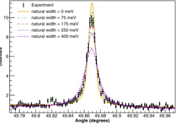
FIG. 10. Example of a dispersive-mode experimental spectrum for the Be-like Ar 1s2s22p1P
1→1s22s2 1S0transition (black dots), together with a few plots of the function in Eq. (1), for different values of the natural line widthŴi
L. The four parameters have been adjusted to minimize the reducedχ2(Ŵ
L) (see text for more explanations).
that the highest p value for the three considered data sets is for n=0, and, as before, one can see a local maximum when considering all experimental results from TablesVIIand
VIIIor just thewlines for the samenvalue as from Fig.8. Considering the standard significance level of 0.05 to evaluate the acceptance or rejection of the null hypotheses (i.e., the fact that the data can be described by theaZnfunction), and since
the highestpvalue is 1.4×10⁻⁶for the three considered data
sets, the null hypotheses has a very small probability to be true, with the caveats noted in Ref. [154]. We also performed at-student test, which shows thata=0 is the most probable value for alln. Therefore, we conclude that it is highly unlikely that the experiment-theory difference has a dependence inZ of the formf(Z)=aZnfor any givennwith 0n12.
VI. RESULTS AND COMPARISON WITH THEORY FOR THE BE-LIKE 1s2s22p1P1
→1s22s2 1S0TRANSITION
A typical spectrum for the 1s2s22p1P
1→1s22s2 1S0
tran-sition, obtained in dispersive mode, is presented in Fig. 10. The width of the 1s2s22p1P1 in contrast to the He-like case,
has both radiative and nonradiative (Auger) contributions. The radiative part is also heavily dominated by the 1s2s22p1P1→
1s22s2 1S
0 transition. As seen in Table IV, the nonradiative
part is mostly due to three Auger transitions: 1s2s22p1P
1→
1s22s2S1/2, 1s2s22p1P1→1s22p2P1/2, and 1s2s22p1P1→
1s22p2P3/2. The radiative and nonradiative contributions are
TABLE X. Measured and computed natural line width values for the 1s2s22p1P1→1s22s2 1S0 transition in Be-like Ar. All values are given in meV, and estimated uncertainties are shown in parentheses.
Transition Experiment Theory Reference
1s2s22p1P
1→1s22s2 1S0 146 (18) 128 (40) MCDF (this work)
121.4 FAC (this work)
150.9 Costaet al.(2001) [139]
146.8 Chen (1985) [99]
2 4 6 8 10 12 14 16 18 20 measurement number
3091.755 3091.760 3091.765 3091.770 3091.775 3091.780 3091.785 3091.790
Energy (eV)
Transition energy Weighted average Statistical error
σ +
σ
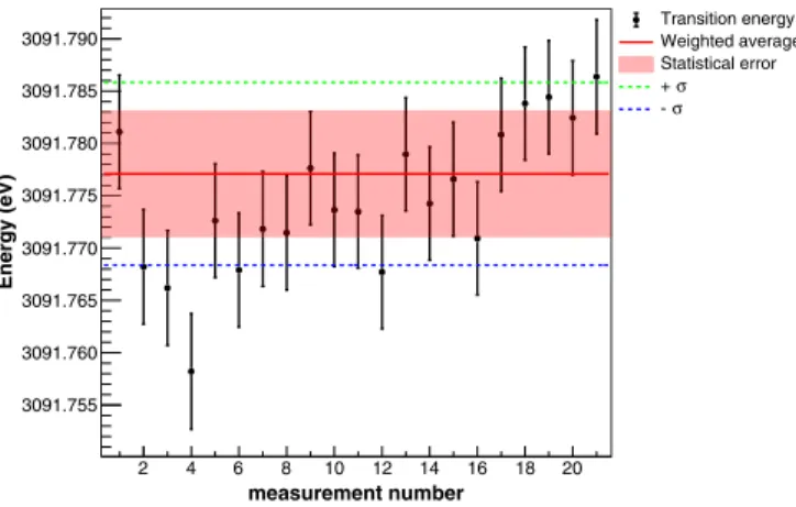
-FIG. 11. Be-like argon 1s2s22p1P
1→1s22s2 1S0 transition en-ergy values for the different spectra recorded during the experiment. Error bars in each point correspond to the quadratic sum of the peak fitting uncertainty with the uncertainties from TableI, which have random fluctuations only, i.e., the angle measurement and the temperature correction. The (pink) shaded area corresponds to the weighted average of the peak position statistical uncertainty obtained from the fit. The±1σlines combine these statistical uncertainties with all systematic errors from TableI. Every pair of points corresponds to one-day data taking (see text for explanations).
of similar size. The distribution of results from the daily experiments is presented in Fig.3(b). Our experimental width and the comparison with theory are presented in TableX. The agreement between theory and experiment is within combined experimental and theoretical uncertainty.
We present in Fig.11the transition energy values obtained from the successive pairs of dispersive and nondispersive-mode spectra, recorded during the experiment for the 1s2s22p1P1→1s22s2 1S0 transition, following the method
presented in Sec.III. The weighted average and±1σ values are plotted as well.
10 15 20 25 30
Z 2.5
− 2 − 1.5 −
1 − 0.5 −
0
E (eV)
∆
Experiment
This work
Ref. [4]
Ref. [42]
Ref. [53]
Ref. [54]
Ref. [56]
Ref. [57]
Ref. [166]
Theory
This work
Ref. [95]
Ref. [96]
Ref. [99]
Ref. [100]
Ref. [168]
Ref. [170]
FIG. 12. Comparison between experimental and theoretical val-ues for the 1s2s22p1P
1→1s22s2 1S0transition energies, as a function of Z. All values are compared to the energies in Ref. [98]. The experimental results are from the following references: Schlesser
et al. (2013) [57], Beiersdorferet al. (1993) [56], Decauxet al.
(1997) [166], Rudolphet al.(2013) [4], Hsuanet al.(1987) [42], Rice
et al.(1995) [53], Riceet al.(2014) [54]. The theoretical results are from the following references: Yerokhinet al.(2015) [96], Yerokhin
et al.(2014) [95], Chen and Crasemann (1987) [100], Chen (1985)
[99], Shuqianget al.(2006) [170], Safronova and Shlyaptseva (1996) [168].
In TableXI, we present our results for the 1s2s22p1P
1 →
1s22s2 1S0 transition energies. The measurement has been
performed with a relative uncertainty of 2.8×10⁻⁶. The
difference with the Yerokhinet al.calculation [96], which is given with a relative accuracy of 11×10−6, is 9.7×10⁻⁶.
The difference with our MCDF results using effective operator self-energy screening is 2.3×10⁻⁶, while it is 3.6×10⁻⁶
TABLE XI. Comparison between experimental and theoretical Be-like argon 1s2s22p1P
1→1s22s2 1S0transition energies. All energies are given in eV, and estimated uncertainties are shown in parentheses.
Transition energy Reference
Experiment
3091.7771(61)(63)(87) This work(stat.)(syst.)(tot.)
3091.776(3) Schlesseret al.(2013) [57]
Theory
3091.716(30)(18)(11) This work using model operators [77,127] (see TableII) (Corr.)(SE screening)(Auger shift) 3091.710 (30)(16)(11) This work using Welton model(see TableII)(Corr.)(SE screening)(Auger shift)
3091.11 This work using FAC [138]
3091.749 (34) Yerokhinet al.(2015) [96]
3088.958 Natarajan (2003) [140]
3091.95 Costaet al.(2001) [139]
3092.157 Safronova and Shlyaptseva (1996) [168]
3090.64 Chen and Crasemann (1987) [100]
3090.66 Chen (1985) [99]
3092.18 Safronova and Lisina (1979) [98]
TABLE XII. Comparison between relative measurements from Ref. [57], and the values deduced from this work and our previous measurement of the 1s2s3S
1→1s2 1S0M1 transition [2] for the 1s2p1P1→1s2 1S0and the 1s2s22p1P1→1s22s2 1S0transitions. All energies are given in eV, and uncertainties are shown in parentheses.
Experiment Theory
Level This work, Ref. [2] Ref. [57] Refs. [59,96] This work
1s2p1P
1 35.432(10) 35.419(11) 35.4337(4) 35.434
1s2s22p1P
1 −12.383(11) −12.372(3) −12.399(34) −12.403
with the calculation using the Welton method. The difference between the present reference-free measurement and the rela-tive measurement presented in Ref. [57], calibrated against the theoretical value of the 1s2s3S1→1s2 1S0 transition energy
of [59] is only 0.4×10⁻⁶. All recent measurements and
calculations are thus forming a very coherent set of data. The energy of this transition has not been extensively studied. It was measured relative either to theoretical values in S, Cl, and Ar [57], Sc [53], Fe [56,166], Ni [42], and Pr [47] or to K edges in Fe [4]. The width and Auger rate for this transition have also been measured in iron [4,167], with the combined use of synchrotron radiation and ion production with an EBIT. In Fig. 12, we present a comparison between theory and experiment, and between different calculations for the 1s2s22p1P1→1s22s2 1S0line energy, for 10Z29.
Since there is no recent calculation covering all elements for which there is a measured value, we use as reference the old calculation from Ref. [98], which does not include accurate QED corrections.
To conclude the discussion on both transitions measured here, we have subtracted the 1s2s3S1 →1s2 1S0M1 transition
energy measured with the same method in Ref. [2] from the energies of the 1s2p1P1→1s2 1S0 and the 1s2s22p1P1 →
1s22s2 1S
0 transition energies measured here (Table XII).
The agreement with the relative measurements performed in Ref. [57] is within combined error bars. The difference between the reference-free transition measurements are in even better agreement with theory than the direct measurements reported in Ref. [57].
VII. CONCLUSIONS
In the present work, we report the reference-free measurement of two x-ray transition energies and widths in He-like (1s2p1P1→1s2 1S0) and Be-like
(1s2s22p1P1 →1s22s2 1S0) argon ions. The measurement of
the 1s2s22p1P1→1s22s2 1S0 transition energy is the first
reference-free measurement for a transition of an ion with more than two electrons. The measurements were made with a double-crystal spectrometer connected to an ECRIS. The data analysis was performed using a dedicated x-ray tracing simulation code that includes the physical characteristics and geometry of the detector. The energy measurements agree within the error bars with the most accurate calculations and with other recent measurements. The measurement of the He-like transition is one of the five measurements with a relative accuracy below 1×10⁻⁵. The measurement of the
Be-like Ar transition is the first reference-free measurement
on such a transition, and the only one with this level accuracy, except for measurements relative to nearby He-like transitions. We have also performed MCDF calculations of the transi-tion energies and widths, using both theMCDFGMEcode, with improved self-energy screening and the RCI flexible atomic code FAC and compared with all existing theoretical and experimental results available to us. TheMCDFGMEtheoretical results are in agreement with existing experimental results and with the most advanced calculations available.
We have analyzed the difference between all availablen= 2→n=1 experimental transition energies in He-like ions forZ12 and the theoretical results from Ref. [59]. When taking into account the recent high-precision, reference-free measurements in heliumlike argon [1,2,7] and the present result, in He-like iron[4], and in He-like krypton[9] from the Heidelberg and Paris groups, as well as the copper result [8] by the Livermore group, we have shown that there is no significant Z-dependent deviation between the most advanced theory and experiment.
The method presented here will be extended to other charge states like lithiumlike or boronlike ions, and nearby elements in the near future.
ACKNOWLEDGMENTS