1
“T
HE
D
ETERMINANTS OF
N
ET
I
NTEREST
M
ARGINS
&
N
ET
I
NTEREST
S
PREADS
I
N
T
HE
R
USSIAN
&
J
APANESE
C
OMMERCIAL
B
ANKING
S
ECTORS
”
Department of Finance
MSc Financial Economics & MSc Finance Master Thesis
by Bora Sentürk
Study Program: Double Degree Program Maastricht Student ID: 6101525
Supervisor: Sun Hang Nova Lisbon Student ID: 23287 Supervisor: Jose Neves De Almeida
2
“The Determinants of Net Interest Margins & Net Interest Spreads in the Russian & Japanese Commercial Banking Sectors”
By Bora Sentürk
ABSTRACT
This study presents an empirical investigation of the determinants of net interest margins and spreads in the Russian and Japanese banking sectors with a particular focus on commercial banks. Net interest mar-gins and spreads serve as indicators of financial intermediation efficiency. This paper employed a bank-level unbalanced panel dataset prolonging from 2005 to 2014. My main empirical results show that bank characteristics explain the most of the variation in not only net interest margins but also in spreads. Capi-talization, liquidity risk, inflation, economic growth, private and government debt are important determi-nants of margin in Russia. In Japan to the contrary loan and deposit market concentration along with bank size do predominate. Common significant variables in both countries are the substitution effect, cost effi-ciency and profitability. Turning to net interest spreads, micro- and macro-specific variables are the main significant drivers in Russia. I reach the conclusion that there are no significant determinants of net interest spreads in Japan within the original selection of variables, but operating efficiency and deposits to total funding seem to prevail. In both countries, there are solid differences in the net interest margins as well as spreads once the pre- and the post-crisis periods are considered.
3 Table of Contents
1. INTRODUCTION ………..6
1.1 Definition of Commercial Banks………...6
1.2 History of Commercial Banking………....6
1.2.1 Russia……….6
1.2.2 Japan………..7
1.3 Why Russia & Japan?...8
1.4 Contribution……….11 1.5 Sub-Questions………..13 1.6 Hypotheses………...14 2. LITERATURE REVIEW………..15 2.1 Dependent Variables………15 2.2 Independent Variables……….16 2.2.1 Bank-Specific Variables………..16 2.2.2 Market-Specific Variables………...19 2.2.3 Micro-Specific Variables……….20 2.2.4 Macro-Specific Variables………20
2.3 Additional Variables for Robustness Testing Purposes……….………..21
3. DATA & METHODOLOGY………..………. 23
3.1 Information about Data………23
3.2 Dependent Variables………24
3.3 Independent Variables……….26
3.4 Expected Impacts……….27
3.5 Methodology………28
4. OVERVIEW OF RUSSIAN & JAPANESE COMMERCIAL BANKING SECTORS…...32
5. EMPIRICAL RESULTS………...45
5.1 Panel Regression Results for Russia………...46
5.2 Characteristic Group Results for Russia ……….61
5.3 Robustness Test Results for Russia……….……63
4
5.5 Characteristic Group Results for Japan………..……….72
5.6 Robustness Test Results for Japan………...73
5.7 Empirical Findings & Limitations of Study………75
6. CONCLUSION………...………...78
7. BIBLIOGRAPHY………..79
APPENDIX………...……….87
Tables
Table 1: Hypotheses & Significance Level Thresholds Table 2: Dependent Variables
Table 3: Bank-Specific Variables Table 4: Market-Specific Variables Table 5: Micro-Specific Variables Table 6: Macro-Specific Variables Table 7: Expected Impacts
Table 8: Additional Variables for Robustness Testing
Table 9: Expected Impact: Additional Variables for Robustness Testing Table 10: Russia Full Dataset: Panel Regressions
Table 11: Russia Full Dataset: Panel Regressions Excluding Foreign Banks
Table 12: Russia Full Dataset: Panel Regressions Excluding Foreign Banks & State Banks Table 13: Russia Full Dataset: Net Interest Margin & Net Interest Spread (Characteristic Groups) Table 14: Russia Full Dataset: Net Interest Margin & Net Interest Spread (Robustness Tests) Table 15: Japan Full Dataset: Panel Regressions
Table 16: Japan Full Dataset: Net Interest Margin & Net Interest Spread (Characteristic Groups) Table 17: Japan Full Dataset: Net Interest Margin & Net Interest Spread (Robustness Tests)
5 Figures
Figure 1: Net Interest Margins & Net Interest Spreads
Figure 2: Net Interest Margins & Net Interest Spreads (Means & Medians) Figure 3: Total Assets
Figure 4: Total Assets of 4 Largest Commercial Banks in 2014 Figure 5: Total Loans & Total Customer Deposits
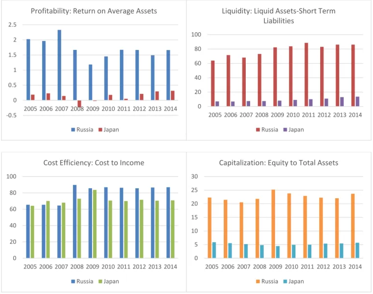
Figure 6: Banking Sector Development (2005-2014) Figure 7: Key Financial Ratios
Figure 8: Overview on Macro- and Microeconomic Conditions
Appendix
Table 1: Correlation Matrix: Russia & Japan
Pre-Word
Motivation
Academic Motivation: Considering both countries, there are many differences including geography, Jap-anese historic links to Russia`s government-driven economic development, industrial structures marked by large oil companies in Russia and “Keiretsu” business networks in Japan. Both have a bank-based financial system and adopted the so-called “German-Japanese model”, however both are at different de-velopment stages and clearly the bank market concentration is also distinct, which can be seen thanks to the Lerner Index for both countries found on the Economic Research site of the Federal Reserve Bank of St. Louis. With this topic, I would like to look into whether those general differences in the commercial banking sectors while attaching a precise importance to net interest spreads (the spread between deposit and lending rates) and to net interest margins.
6 1. Introduction
1.1 Definition: Commercial Banks
Commercial banks take deposits and lend money to private and corporate clients, including SMEs and organizations. Services cover current, deposit and saving accounts.1 Commercial banks earn income by taking in small, short-term and liquid deposits and engage in asset and maturity transformation in order to give out larger loans with longer maturity to clients. While retail lending involves high volumes and low value loans, the wholesale lending includes other banks, pension funds and corporations as borrowers, comprising low volumes of loans, but those loans tend to have high values. The separation between com-mercial and investment banking has been becoming weaker amid the era of financial liberalization and globalization between 1990 and 2007. Banks have been observed to move from low margin deposit-taking and loan business to the higher margin capital market business, as a consequence increasing the risk of commercial banks. Moving to riskier but potentially more profitable loans is an option, but also scooping up bond and equity issues at the expense of bank loans. In the United States, the Gramm-Leach Bliley Act repealed key provisions of the Glass-Steagall Act, known for the separation of commercial and investment banking. After the recent financial crisis, the Volcker Rule disallowed proprietary trading of securities for all deposit-taking institutions.2
1.2 History of Commercial Banking 1.2.1 Russia
Wladimir I. Lenin annotated that the control, which commercial banks had reached over individual indus-trial companies led to the concentration of production. He assigned the banks' capability to execute this control mostly to industry's dependence on them for receiving both additional equity capital and credit. Lenin noticed their “potential for central control and direction of dispersed industries in a country where regional and local units of the government's administrative apparatus were inadequate to deal with eco-nomic problems”3. He was awed by the technical operative performance by the wide branch networks prevailing the scene in Germany, the United Kingdom, France, and Russia itself, rather than with the opportunity of the use of monetary and credit policy as a tool for economy restructuring and achieving appropriate economic growth and stability. After the October Revolution in 1917, the Soviet government
1http://www.investopedia.com/terms/c/commercialbank.asp 2http://lexicon.ft.com/Term?term=commercial-bank
7
pushed through with nationalizations of all commercial banks without compensation of domestic or for-eign stockholders by suspending all their shares. The commercial banks were joint into the State Bank, whose name was changed to People's Bank (Norodny Bank) of the Russian Socialist Republic. The re-markable side of the Soviet banking system lies, rather, in the whole integration of monetary processes within the central planning system, along with the credit and foreign exchange monopoly of the State Bank that has a wide set of control powers over the performance of the entire state-owned segment. His-torians view the position of the State Bank of the U.S.S.R. (Gosbank) today as the definite expression of a relationship between government and banking that originated in Tsarist Russia. In the beginning of 1992, the country initiated its economic reform process, the goal of which was to transform the formerly cen-trally managed economy into a market economy. In 1988, it was permitted to found commercial and co-operative banks, one of the strong underlying pillars to support the market economy.4
1.2.2 Japan
The significance of zaibatsu dominance in commercial lending activity is emphasized by the relative ir-relevance of private saving and security buying transactions by individuals in Japan. Zaibatsu is the Jap-anese term for industrial and business conglomerates that ruled substantial segments of the economy in the Empire of Japan from the Meiji Period (1968 – 1912) until the end of World War II. The zaibatsu created their own banks that had the task to finance activities of its group member companies. The zaibatsu banks retained the deposits of affiliated companies and ranked at the same time among their principal sources of capital. The zaibatsu system impeded business outside zaibatsu control to obtain investment funds for much worse terms as applied to those within the group.
Pre-War Japanese banks numbered not among institutions that conducted large, long-term investments in companies. Instead, they considered themselves as commercial banks that specialized in assorted payment functions and short-term loans. During the war, the government gradually pushed commercial banks to-wards supplying long-term funds to munitions firms. M. Ogura, the former Japanese Finance Minister in 1941 presented that the government would want banks to commit themselves in so-called “enterprise fi-nance” to provide long-term funds for expansions in productive capacity.5 After the zaibatsu era, the new
“keiretsu” era began which had the upper hand on the economy in the second half of the 20th century,
above all during the “Japanese Economic Miracle”. Keiretsu stands for a whole slew of companies with
4 http://www.suomenpankki.fi/fi/julkaisut/selvitykset_ja_raportit/yleistajuiset_selvitykset/Documents/74015.pdf 5 http://www.law.harvard.edu/programs/olin_center/papers/pdf/289.pdf
8
interlocking business relationships and shareholdings, complementing an informal business group. The cross-shareholdings system aids to isolate from takeover endeavors, facilitating long-term planning in order to push forward with innovative projects such as the ones in the electronics and automotive indus-tries.
While in Russia, state-owned banks and large banks, which constitute a small percentage of the entire commercial banking sector are protected by the government, in Japan the interconnectedness and the de-veloped depth of the financial system makes many banks relevant for government safety nets. If a small bank goes bankrupt during the consolidation process as it has been happening in the Russian commercial banking sector, it will not put the entire economy at stake. This is different in Japan, where there are larger, more connected banks within the keiretsu networks linking banks, large corporations, insurance compa-nies, manufacturing entities with each other very closely. The potential danger to the real economy is thus a lot more considerable than in Russia. Keiretsu, the main banking system coupled with close cooperation with the Japanese government, reduces the financial risk. Not only the relationship to the government, but also the inter-company relationships within the keiretsu networks is very important. Banks give out loans to their fellow keiretsu companies, which enables them to reduce information asymmetry and make mon-itoring more effective, resulting in lower borrowing rates. These keiretsu networks do provide the property of risk-sharing, facilitating therefore more risky, long-term, low margin investments. The Japanese gov-ernment has been known for enabling funds and necessary capital in the form of financial support and guarantees. The Ministry of Finance (MoF) has developed in the past various formal and informal ap-proaches to prevent bank failures. The implicit blanket protection and the convoy system instead of simply the reliance on the deposit insurance system serve as examples. The convoy system centers upon the MoF`s encouragement of stronger, more robust banks to be capable to absorb insolvent banks. Effectively seen, all banks are tied to each other. Financially problematic banks are picked up by stronger banks, giving an incentive to the government not to push through necessary reforms in the financial sector.6
1.3 Why Russia?
First, the Russian banking system has been subject to important structural changes and experienced fast development of its banking sector. Financial deepening has been also a factor to this evolvement. Second, the income structure and balance sheet dynamics of Russian commercial banks have seen major shifts, especially when it comes to the transition from margin income to non-interest fee-based income. Third,
9
even though the financial development in Russia is underway quickly, it remains on low levels compared to developed countries such as Japan.
Most significant progress in the Russian banking sector manifested itself in the era of Russian President Boris Yeltsin. The Russian government announced all branches of all-union banks in Russia to be inde-pendent from the Gosbank – which had been the Central Bank of the Soviet Union. The result of this declaration was that almost 1,000 new banks came into existence overnight. After the independence of all banks, another step was taken to ensure the transformation of more than 900 regional branches of special-ized banks to independent entities as well. These decisions laid the foundation for a competitive market within the banking sector. By the end of 1996, the total number of banks was about 2,100, while the year after this number decreased rapidly to 1,700 banks and in 2001, there were 1,300 banks. In 1993 the capital requirement to start a bank was about USD100,000. This very low amount led to a strong presence of Russian entrepreneurs starting banks.7
Unfortunately, in Russia there seems to be a big difference between the formulation of laws and the exe-cution of those laws by government officials. The cost of regulation and bureaucracy keeps foreign banks far away from entering the Russian market, thus leading to the non-materialization of liberalization re-forms. State-support for selected Russian competitors with good political connections does not provide a healthy and fair environment for foreign banks to do business in. Government interventions influence lending decisions, too. The government declared during the crisis in 2009 that additional government capital injections in individual banks would have to be in accordance with the banks` agreement and com-pliance with specific government-given lending targets. Despite a high number of banks, there is little competition within the banking sector so that it represents a major impediment for efficient capital allo-cation. The majority of the banking sector is made out of small banks, which lack risk management and control capabilities, cannot benefit from economies of scale and are in desperate need of a greater depos-itor base. The vulnerability to oil prices in general is another layer of difficulty those banks face. This condition leads those banks to provide only the private sector with small and short-term loans, which in turn also hurt and challenge Russian SMEs. The conclusion on behalf of the Russian banking reforms rest on the government`s reform overpromising, but the reality is that the government considerably under-delivers. What is on paper does not comply with actions and execution.
10
Despite the underperformance of banking reforms, there has been progress indeed. While Russia was suffering a substantial gap of about 10% between gross savings-to-GDP and domestic private sector in-vestment in the period of 2000-2012, the situation has improved. The mean gap during our sample period from 2005-2014 has shown a much lower number of 5.71%, even though it is twice as high as Japan`s. While the gap in Russia was at 11.13% in 2005, in 2014 it had moved below 2%. The Russian problem of recycling savings into investments has been working better than before. Moreover, the adoption of inter-national accounting standards of Russian banks in 2004 and the implementation of deposit insurance to every bank in Russia has helped to create the necessary basic structures to develop the financial sector. Financial intermediation has developed fast over time, whether it is in terms of banking assets, loans or deposits relative to GDP or in terms of M2/GDP, an indicator of financial deepening. Stock market capi-talization to GDP has been growing strongly and reached a level of more than 50% in 2014, while in Japan the same figure stands at slightly below 70%. Even outstanding debt securities, including both domestic and international, relative to GDP, accomplished a level of 6% in 2011, however growth has been slow, finding itself in a stable upward trend. In Japan, this figure is much higher at almost 58%. The Russian bond market is not greatly developed, since only a handful of huge Russian conglomerates issue bonds. The role of bank loans though, gives reason to be optimistic. Bank loans as a source of corporate financing of fixed investments has ascended from only 2.9% in 2000 to more than 9.3% in 2013. Even though the absolute percentage level is truly low, growth has proved itself to be firm.
Why Japan?
Japan has created an alternative financial system model to the Anglo-American market-based system, which is called the bank-based “Japanese-German model”. This model has been implemented by Russia during its current transition and development of its banking sector. Due to the significant fixed cost of underwriting securities, the market-based model is much more expensive or even completely inaccessible to SMEs compared to bank loans. The cost of underwriting becomes proportionally larger the smaller the amount of financing needed. Another crucial reason is that big portfolio investors may not want to invest in companies of limited size, as the costs of screening and monitoring are also fixed, and make small investments unprofitable. A bank-based system is, thus backed by economies with large parts of SMEs and highly indebted firms according to Vitols (2002)8. Indeed, in Japan private sector debt has been 168%
relative to GDP in 2014 with a mean over the sample period from 2005 to 2014 of 171% of GDP, while
11
the mean of Russian private sector debt had reached a considerably lower percentage of only 49% of GDP since it is a developing economy still. SMEs have been becoming more dependent on financing from banks, as more intense competition has eaten up profit margins, which in turn resulted in a weaker posi-tioning of self-financing investments and daily operations. Japan`s bank-based system is now slowly shift-ing towards a more Anglo-American style of market-based finance, and the reasons for this emergence are the following: First, the government bond market might have the potential to become a key competitor to banks, so that a light level of government debt can support bank-based systems rather than a high level of government debt. This competition comes into appearance due the fact that households and investors might prefer bond securities over deposits, since the government has a higher probability of repayment due to its tax revenues. Furthermore, banks might invest in government securities rather than investing in higher risk assets such as loans. Japan`s government debt to GDP has had a mean during the aforemen-tioned period of 200%, while Russia`s was much lower at slightly above 18%. Secondly, large conglom-erates and firms that have had success in bringing their debt levels down turned to markets in order to receive cheaper sources of finance than bank loans. However, the majority of Japanese companies is highly indebted and needs continued financial backing by banks so that they are able to roll over financing. Thirdly, population growth in Japan has turned negative. Japan is found among the countries with the oldest population in the world. Hence, Japanese pension funds have been carrying on to drive the transition towards a more market-based system with domestic and international investment funds and tools to gain different sets of risk-returns in portfolio management to capitalize on them. But, also Russia`s population growth is weak and is expected to turn negative in the upcoming years.
Outstanding debt securities issued by banks to GDP in Japan shot up from 33% in 2005 to 58% in 2014, while in Russia this percentage rose from 0.02% to 5.09%. Total Domestic debt securities outstanding from all issuers based in Japan rose from 205% to 260%, whereas the Russian figure more than doubled during the sample period from 6% to 13%, but remains at low levels. To sum up, Japan`s bank-based financial system is shifting towards more market-based finance, especially seen among the large compa-nies and the public sector. In contrast, this cannot be said for households and SMEs, where bank finance remains their lifeblood.
1.4 Contribution
My main contribution is twofold. When it comes to this topic, many academic papers focus on a large group of countries or specialize in frontier markets, especially those located on the African continent as
12
elaborated by S.B. Naceur & M. Goaied (2008) with the example of Tunisia9. These papers do neither have an explicit comparison of pre- and post-crisis periods of the recent crisis. Furthermore, my work will be more concrete in developing a precise Asian case by comparing Japan with Russia. Clearly, at first glance, the Japanese and Russian economies are different, especially Japan being a fully developed econ-omy while Russia belongs to the BRIC emerging markets. Both economies are ranked among the top 10 largest economies in the world (by GDP size) according to the World Bank 2014 GDP size ranking.10 Japan is the third largest, while Russia is the tenth largest economy.
According to Vladimir Popov`s academic paper: “Financial System in Russia as compared to other tran-sition economies: Anglo-American versus German-Japanese model”, both Russia and Japan belong to the bank-based German-Japanese financial system model, rather than the market-based Anglo-American model.11 However, my study will contribute to figure out which differences and similarities exist when taking a look at the commercial banking sectors and the financial intermediation dynamics therein, despite both countries belonging to the same financial system model. My paper will shed light on this issue in a more detailed way than the general descriptions and explanations of Popov`s work. An additional contri-bution of my paper will be a very specific comparison between both countries, which in the existing liter-ature can be found in an extremely limited range. The available empirical papers concentrate either on the analysis of 20 up to 100 countries or on particular continents or regions such as Latin America, Central & Eastern Europe, the European Union, East Asia, Central Asia & the Caucasus that can be found for exam-ple in the analyses composed by L.M. Tin et al. (2011)12, M. Dumicic & T. Ridzak (2013)13, R. Almarzoqi & S. B. Naceur (2015)14, J. Maudos & J.F. Guevara (2004)15. Another common focus of literature is the attachment of importance to one country only such as in L.R. Sidabalok & D. Viverita (2012)16, P. Sharma & N. Gounder (2012)17, D. Estrada, E. Gomez, I. Orozco (2006)18, E. Bektas (2014)19. My work
9 http://papers.ssrn.com/sol3/papers.cfm?abstract_id=1538810 10 http://databank.worldbank.org/data/download/GDP.pdf 11 http://fir.nes.ru/~vpopov/documents/FINSYS.pdf 12 http://papers.ssrn.com/sol3/papers.cfm?abstract_id=1912319 13 http://hrcak.srce.hr/97824?lang=en 14 https://www.imf.org/external/pubs/ft/wp/2015/wp1587.pdf 15 http://www.uv.es/maudosj/publicaciones/JBF.pdf 16 http://papers.ssrn.com/sol3/papers.cfm?abstract_id=1990175 17 http://papers.ssrn.com/sol3/papers.cfm?abstract_id=2089091 18 http://www.banrep.org/docum/ftp/borra393.pdf 19 http://businessperspectives.org/journals_free/bbs/2014/BBS_en_2014_04_Bektas.pdf
13
tiates itself from the others by having implemented two countries in a comparison setting along with pos-sible explanations and interpretations for the generated regression outputs, which is clearly an advantage over those papers that compare multiple countries, limiting the ability and the space to elaborate on certain explications. From a practical point of view, my study will be relevant in order to give readers an insight into the commercial banking and financial intermediation dynamics in Asian countries such as Russia and Japan. Furthermore, it will also offer policymakers a foundation for debate, since my study will highlight the significant determinants of margins and spreads. Once those are known, they can advance by thinking further about reforms that make financial intermediation even more efficient. Financial intermediation is the lifeblood of investments, consumption, wealth and growth of economies. This is why profound anal-yses and studies are crucial in this field.
This study is structured as follows: Section 2 provides a summary of related literature with respect to the main introduced dependent and independent variables. Section 3 deals with the empirical methodology and comments on the data. Section 4 explains the major developments in the Russian and Japanese com-mercial banking sectors over the last 10 years. Section 5 combines the empirical results with an extensive discussion and presents interpretations of the results. The last section concludes with the major take-away of this study.
1.5 Sub-Questions
a.) Is there a pro-cyclicality in the determinants of net interest margins and spreads from before 2008 and afterwards?
b.) Among bank-specific, market-specific, micro – and macroeconomic variables: Which group explains the variation in net interest margins and spreads better?
c.) How does inflation and competition influence margins and spreads?
d.) Which are the common variables being significantly responsive to margins and spreads in both an emerging market like Russia and in a developed economy like Japan?
e.) Which variables have to be taken into account the most by policymakers in order to increase the effec-tiveness of their reforms in light of the intended financial development process, including the reduction in spreads for allowing a more efficient financial intermediation?
14
f.) Russia adopted a decentralized banking system, whereas most economies in transition, including radi-cal reformers, adopted a more conservative Japanese-European type being a highly concentrated model of the banking sector. Is this difference having an economically and statistically significant effect on the determinants of net interest margins and net interest spreads in Russia and Japan?
g.) Russia`s banking system has been developing quickly. Does this automatically mean that Russia is becoming more and more similar in its financial intermediation dynamics compared to the developed banking system of Japan? Have they reacted differently in pre- and post-crisis period of 2008 making the relevant implemented dummy significant?
1.6 Hypotheses
In order to be able to answer the aforementioned sub-questions correctly, I set up hypotheses with refer-ence to the individual variables, which I believe to be of great help in understanding the dynamics in financial intermediation and the decisive and more importantly most responsive factors. The relevant null and alternative hypotheses are listed below. The significance level applicable to this statistical hypothesis testing is determined to be α=10% which is the critical probability threshold deciding whether to either reject the null hypothesis in favor of the alternative one or not to reject it. The decision rule is based on the null hypothesis being rejected if the observed value of the regression output is located in the critical area, and fails to reject if the null hypothesis is otherwise.
Table 1
Hypotheses & Significant Level Thresholds
Null & Alternative Hypotheses for considered dependent variables along with the significance level threshold of 10%
Variable Null Hypothesis Alternative Hypothesis Significance Level Threshold
Size H0: µ=0 HA: µ≠0 10%
Profitability H0: µ=0 HA: µ≠0 10%
Liquidity Risk H0: µ=0 HA: µ≠0 10%
Substitution Effect H0: µ=0 HA: µ≠0 10%
Bank Efficiency H0: µ=0 HA: µ≠0 10%
Risk Aversion & Capitalization H0: µ=0 HA: µ≠0 10%
Herfindahl-Hirschman Index (D) H0: µ=0 HA: µ≠0 10%
Herfindahl-Hirschman Index (L) H0: µ=0 HA: µ≠0 10%
Private Sector Debt H0: µ=0 HA: µ≠0 10%
Government Debt H0: µ=0 HA: µ≠0 10%
Economic Growth H0: µ=0 HA: µ≠0 10%
15 2. Literature Review
Previous literature pointed out factors affecting net interest margins into three components:
The level of market competition and risk (Ho and Saunders, 1981), as well as operating costs (Maudos and Guevara, 2004). The ongoing debate on the driving forces of net interest margins started in a study by Ho and Saunders (1981).20 The authors modeled a deposit-taking bank as a financial intermediary institu-tion. Conclusions of the study present the behavior of banks as intermediaries between borrowers and lenders. The theoretical model shows the optimal bank interest margin depends on four factors: Risk aver-sion, market structure, the average transaction size and the variance of deposit and loan interest rates.
2.1 Dependent Variables
At first glance, net interest margins and net interest spreads might have similar consequences on financial intermediation efficiency. However, the way they are calculated has to be distinguished:
Net Interest Margins: Net interest margins are based on the interest income generated, which includes all
earning assets of the bank (outstanding loans, securities, excess reserves) minus all the interest-bearing liabilities of the bank, which it pays out to its lenders (deposits, loans, bonds) relative to the amount of total assets: NIMi,t = (Interest incomei,t - Interest expensesi,t) / [(Total assetsi,t-1+ Total
as-setsi,t)/2]
Net Interest Spreads: The net interest spread will enable me to refine my analysis on intermediation since
it is the difference specifically between the deposit rates the bank pays its depositors and the lending rates the bank charges on its outstanding loans. The spread also tends to be more sensitive to competition in the banking sector: NISi,t = {Interest received from loansi,t /[(Total loanst-1+ Total loanst) / 2]}–{(Interest paid
on depositst/ [(Total depositst-1+ Total depositst)/ 2]}, where t is the current year, t-1 the previous year and i an individual bank from the dataset. High interest rate spreads contribute to discouraging savers with low returns on their deposits, while charging high interest rates for loans limits financing for potential borrowers and investors. Financial systems in developing nations have been revealing significantly and persistently greater average financial intermediation spreads in comparison to developed nations accord-ing to Hanson and de Rezende Rocha (1986).21 High spreads are known to originate from inefficiency,
20 https://www.imf.org/external/pubs/ft/wp/2014/wp14163.pdf (p. 4-6)
21
16
high risk-taking and lack of competition. High spreads demonstrate advantages and disadvantages. On one side of the coin, high spreads embody the pivotal mechanism through which the banks create profits and by doing this, they shield themselves against credit risk (Barajas, Steiner, Salazar; 1998).22 This mech-anism then leads to a gain in strength and solidifies the banking system. On the flipside, high spreads tend to be a key signal of operating inefficiency. High spreads combined with low concentration have the po-tential to lay the foundation for the wrong incentive of not having to enhance operating efficiency and above all the quality of loans in the portfolio.
2.2 Independent Variables
The dependent variables have been compartmentalized into four groups:
Bank-specific variables: These variables concentrate on the characteristics of individual banks Market-specific variables: These variables concentrate on the influence of the commercial banking
market structure
Micro-specific variables: These variables concentrate on the impact of microeconomic conditions Macro-specific variables: These variables concentrate on the impact of macroeconomic conditions 2.2.1 Bank-Specific Variables
a.) Size: As a proxy of size, I have taken Total Assets. Berger (1995) states that the benefits of
econ-omies of scale and market power allow large banks to remain more stable than their smaller coun-terparties. O`Hara and Shaw (1990) add that executives of bigger banks might have factored in their access to government safety nets put in place to bail out large financial institutions in times of intense distress given their “too big to fail” status quo.23 Ex-ante it is very difficult to determine
the effect of bank size on interest margins. First, a positive relationship might be possible thanks to the expectation that large banks can strengthen the depositor`s perception of its stability and credibility, so that the depositors might agree on accepting lower interest earnings from deposits because of higher perceived safety. This perceived safety may also be linked to large banks having the capability to diversify its activities and lower overall bank risk. As deposit rates are pushed lower, the interest spreads increase (Blaise Pua Tan, 2012).24 On the other hand, Demirgüc-Kunt, Laeven and Levine (2003) illustrate by considering data from 72 countries in the period from
22 http://www.palgrave-journals.com/imfsp/journal/v46/n2/pdf/imfsp199912a.pdf (p.196-197) 23 http://www.gla.ac.uk/media/media_199406_en.pdf p. 11
17
99 an increased probability for large banks to have smaller net interest margins, as they can take advantage of economies of scale.25
b.) Profitability: As a proxy for profitability, I used the Return on Average Assets, whereby the
aver-age assets are not the assets at the end of the year, but the averaver-age assets throughout the respective year. The rationale behind this variable is that the more profitable a bank is, the less risky it is perceived to be by depositors. This is why deposit rates are expected to sink widening the net interest margin and spread.
c.) Liquidity: Liquidity is proxied by the Liquid Assets to Short-Term Liabilities ratio. The utilization
of this ratio is intuitive because the more liquidity the bank has on the side lines, the bigger the opportunity costs of not investing and therefore gaining higher returns on those liquid assets. The comparison of liquid assets to short-term liabilities is relevant because deposits mostly belong to short-term debt. Illiquidity can be caused by the interest mismatch or maturity mismatch. The higher the liquidity ratio, the lower the liquidity risk, but the opportunity cost of holding liquidity rises, resulting in banks charging higher net interest spreads (Nassar, Martinez and Pineda, 2014).26 Banks are liquidity service providers. Since it is possible to create a Pareto optimal condition, it is not possible to fully cover liquidity risk.27 In order to minimize the liquidity risk, it is required to have an efficiently working interbank market.28 However, especially in the case of Russia this is not a given condition and therefore makes liquidity risk a relevancy to deposit holders of individual Russian commercial banks. Liquidity is a potential risk which should not be ignored, above all after the beginning of the financial crisis of 2008/09 when additionally the interbank markets had been under pressure and cost of funding skyrocketed. In pre-crisis periods, interbank markets can serve as a cheap funding source reducing loan rates, but during times of distress, too much of a focus on money market funding can turn out to be very expensive.
d.) Cross-Subsidization: The potential of cross-subsidization within the banks is accounted for by the
Total Non-interest Income to Total Assets ratio. A crucial contribution has been made by Carbo
25 http://www.nber.org/papers/w9890.pdf 26 https://www.imf.org/external/pubs/ft/wp/2014/wp14163.pdf 27 https://www.macroeconomics.tu-berlin.de/fileadmin/fg124/financial_crises/literature/Diamon_Dybvig_Bank_Runs__De-posit_Insurance__and_Liquidity.pdf 28 http://www.nyu.edu/econ/user/galed/archive/Preference%20shocks,%20liquidity%20and%20central%20bank%20pol-icy.pdf
18
& Rodriguez (2007). They developed a model encompassing both aforementioned income streams testing the European banking system. Their result underlines that diversification in non-interest banking activities cause a decrease in the spread due to a potential cross-subsidization effect.29 On
the other hand, Williams and Rajaguru (2010) used panel vector auto-regressions by including Australian banks. Their finding is based on increases in the banks` non-interest income were uti-lized to complement declines in the net interest margin. Even so, the degree of the rise in the non-interest income is punier than the fall in the net non-interest margins. Furthermore they have shown that the growth in non-interest income leapfrog the plummeting in the so-called interest-sensitive margin income, emphasizing the proactivity of Australian banks whilst the process of disinterme-diation.30 Increases in non-interest income not only push up the volatility in profits, but also con-tribute to the worsening of the U.S. banks` risk-return trade-off (DeYoung and Rice, 2004).31
e.) Bank Efficiency: As a proxy, I use the Cost-to-Income ratio in order to get an insight into the
bank`s efficiency. The ratio compares personnel expenses and operating costs to operating income before provisions. It is a measure of how costly it is for a commercial bank to create a unit of operating income in terms of costs. Inefficiency causes higher costs and as a result of this, wider net interest margins and net interest spreads. The higher the ratio, the more inefficient the bank and vice versa. The cost-to-income ratio is computed by dividing operating and personnel expenses by the sum of total net interest income and total non-interest income.
f.) Risk Aversion: As a proxy for risk aversion, I use the Equity-to-Total Assets ratio, whereby the
book value of equity is considered here. The higher this ratio is, the more risk-averse the bank is. A high equity-to-total assets ratio may indeed have different consequences. The higher the ratio the less risky it might be also perceived by depositors who in turn might be satisfied with lower deposit rates, having a positive effect on net interest margins and net interest spreads. At the same time though, the higher risk aversion might lead the bank to invest more of the deposits into less risky loans or even in fixed-income securities with a low risk profile, lowering both net interest margins and net interest spreads. Claeys and Vander Vennet (2008) point out that a higher
29 http://www.ugr.es/~franrod/CarboRodJBF.pdf
30 http://papers.ssrn.com/sol3/papers.cfm?abstract_id=1007166 31 http://papers.ssrn.com/sol3/papers.cfm?abstract_id=487704
19
to-total assets ratio indicates a better credit-worthiness, which ensures lower deposit rates. It also provides the banks with the flexibility to invest in riskier assets with higher returns and higher loan rates. In addition, the findings of their study for Central and Eastern European countries for the period from 1994 – 2001 reveal the positive relationship on the Net Interest Margin.3233 What is more interesting though is that its impact is twice as large for transition economies (to which Rus-sia belongs) than developed countries (to which Japan belongs). Because equity is more costly than deposits, it is likely to be reflected in higher margins.
2.2.2 Market-Specific Variables
g.) Market Concentration: is captured by the Herfindahl-Hirschman Index (HHI). The HHI is
calcu-lated by taking the sum of squares of individual deposit market and loan market shares of all op-erating commercial banks: HHI = (MS1)2 + (MS2)2 + (MS3)2 + (MS4)2 + … + (MSt)2 , where t refers to the respective year. The HHI ranges between 0 and 10,000, whereby 0 implies perfect compe-tition and 10,000 means that an individual bank having 100% of the market share.34 The U.S. Department of Justice, for example, avails itself of a benchmark of 1,000. Results below that benchmark indicate a competitive market, whereas results of 1,000 to 1,800 demonstrate a mod-erately concentrated market as confirmed by Twomey, Green, Neuhoff, Newbery (2005).35 I ap-plied the HHI on two underlying markets: The deposit and the loan markets. More concentration in either of the markets may increase market power and eventually lead to higher margins and spreads. Turk Ariss (2010) demonstrates that different extents of market power do have implica-tions on bank efficiency and risk in developing countries.36 The climb in market power tends to result in two outcomes: Firstly, it increases bank risk. Secondly, it increases profit efficiency. Mau-dos and Guevara (2004) came up with an extension of Ho and Saunder`s theoretical model by considering operational costs as a determinant of net interest income, and based their estimations on the European banking sector over the period of 1992-2000. Moreover, they included market
32 http://papers.ssrn.com/sol3/papers.cfm?abstract_id=1260861 33 https://www.imf.org/external/pubs/ft/wp/2013/wp1334.pdf 34 http://www.investopedia.com/terms/h/hhi.asp 35 http://web.mit.edu/ceepr/www/publications/reprints/Reprint_209_WC.pdf (p. 17-20) 36 http://www.researchgate.net/publication/46497233_On_the_Implications_of_Market_Power_in_Banking_Evi-dence_from_Developing_Countries
20
forces (market power) by using the Lerner Index as a proxy for market concentration. Their result is that an increasing index of market concentration has positive effects on net interest margins. 2.2.3 Micro-Specific Variables
h.) Private Sector Debt: The variable is Private Sector Debt to GDP, which takes into account only
the debt of non-financials and households, but not of financial corporations. The financial corpo-rations are not included, since a large part of them are commercial banks. The leverage of banks is taken care of by the variable equity-to-total assets ratio on the bank level. They are not included due to a high likelihood of significant correlation between these variables. Companies might be overleveraged, decreasing the flexibility of them to obtain new loans. If loans are provided, interest rates might be too high. Banks might be also risk-averse and not willing to lend at all. The riskier the loans, the higher the lending rates, thus the higher the intermediation spread.
i.) Government Debt: As a proxy, I implement Government Debt-to-GDP ratio. Government deficits
that have to be financed by domestic resources might be an opportunity for the banking system for a relative safe investment of their deposit base, thereby driving up lending rates and reducing the amount of financial resources channeled to private sector credit. This might crowd out credit to the private sector. Especially, for a country like Japan, which has the highest government debt-to-GDP ratio in the world according to the International Monetary Fund and World Bank37, this var-iable is relevant to check upon. Tennant and Folawewo`s (2009) research on 33 countries validate my assumption of relevancy of this variable.38
2.2.4 Macro-Specific Variables
j.) Real GDP growth per capita: Usually what is observed in the banking industry is the
pro-cycli-cality of lending, meaning that banks tend to lend more during economic booms, are very careful and tighten their lending standards once the economy experiences a bust or sluggish growth (Ber-ger & Udell 2003).39 In order to have a more precise understanding of GDP growth and due to the
fact that in both countries Russia and Japan, population growth has been a negative trend, I use
37 http://data.worldbank.org/indicator/GC.DOD.TOTL.GD.ZS
38
https://www.centralbank.org.bz/docs/rsh_4.5_conferences-working-papers/determinants-of-interest-rate-spreads-in-belize.pdf?sfvrsn=4 (p.13-14)
21
GDP per capita. In Bernanke and Gertler`s (1989) study paper, it was highlighted that borrowers` creditworthiness worsens together with their net worth (as asset prices tumble and adversely affect collateral values) during recessions. The outcome is that banks either stop lending or lend at high interest rates.40
k.) Inflation: Research conducted by Brock and Rojas (2000)41 suggests that inflation indeed
contrib-utes to spreads. Rising inflation is reflected in the high bank intermediation margins consequently. Elevated inflation has the potential to blur decision-making on bank level, deteriorate information asymmetry and drive price volatility. Inflation means economic uncertainty and hence tends to enlarge margins. An important remark, though, is that the rate on the liabilities can also adjust quicker than the interest rate on the asset side of banks (Claeyes and Vander Vennet, 2008), leading to a negative relationship between inflation and the spread.
2.3 Additional Variables for Robustness Testing Purposes
l.) Population growth: Population growth might not only drive GDP growth, but also deposit growth.
The more people there are, the more deposit accounts should be opened. This contribution to a greater deposit supply may have the potential to drive down deposit rates and at the same time increase net interest spreads. Another option could be that the larger the population, the more lend-ing to households and firms there will be, allowlend-ing more diversification in the loan portfolios of banks, reducing risk and thus lowering deposit rates. The lending rates are expected to be driven higher as well due to a pick-up in credit demand.
m.) Money Supply growth: Real money supply M2 is taken into consideration as a variable, which is
indicative of financial development and financial deepening of the country. According to Ciftcioglu & Almasifard (2015)42 work paper and the World Bank43, it is the degree of monetiza-tion. A lower degree of monetization implies a lower extent of the financial system`s development that may represent a subsequent lower level of efficiency in intermediation services reflecting greater spreads. According to the Money Supply Rule presented in Carlin and Soskice`s book
40 http://www.nber.org/papers/w2015.pdf
41 https://jsis.washington.edu/latinam/file/BrockRojasBankSpreadsJDevpEcon2000.pdf 42 http://jedsnet.com/journals/jeds/Vol_3_No_2_June_2015/1.pdf
22
(2006)44, growth of money supply determines the rate of inflation in the medium-run equilibrium. Since, by definition of the medium-run equilibrium, inflation is constant, the real demand for money is constant, too. The consequence of the requirement that the money market is in equilib-rium is that the real supply of money must also be constant. To keep the real money supply constant, the price level must increase at the same rate as the nominal money supply that is under the control of the central bank. The medium-run equilibrium is marked by a constant inflation rate being equal to the constant growth rate of the money supply set by the central bank. When operating a monetary rule, the central bank`s operations have to guarantee that the money market is in equilibrium, oth-erwise the interest rate would not remain at the desired level and start moving up or down.
n.) Operating Efficiency: The proxy used is the Operating Expenses-to-Total Assets ratio. The higher
the operating costs relative to total assets, the higher the inefficiency, thus the wider the spread in order to cover those costs. Gerlach, Peng and Shu (2005) tested 29 retail banks in Hong Kong during the period between 1994 and 2002 and found out that there is a pass-through effect of operating costs to the interest spread.45 Furthermore, Doliente (2005)46 and Demirgüc-Kunt and Huizinga (1999)47 findings are based on their conclusion that there is at least a part of operating costs transferred to the net interest spread.
o.) Credit Risk: The proxy for credit risk is the Total Credit Reserves-to-Total Loans. The primary
proxy used for credit risk in other academic papers is non-performing loans. Owing to the lack of an ample amount of data, I am not able to proxy credit risk by the ratio of non-performing loans to total assets. The rationale behind credit risk is that the more credit reserves relative to loans are held, the more opportunity costs there are which are likely to be, at least partially, forwarded in the form of a wider spread.
p.) Specialization in Loan Business: The ratio of Loans-to-Total Assets, implying the specialization
in loans, may have a positive relation to bank risk. The intuition behind this is that the greater the exposure to loans is, the higher the likelihood of default risk according to Liu (2010)48. In case of
44 Macroeconomics: Imperfections, Institutions & Policies (Carlin & Soskice), p. 81-96 45 http://www.bis.org/publ/bppdf/bispap22x.pdf
46 http://www.cba.upd.edu.ph/phd/docs/jsd_afel.pdf
47 http://www.dnb.nl/binaries/Working%20Paper%20387_tcm46-295326.pdf (p.21 – 22) 48 http://www.gla.ac.uk/media/media_199406_en.pdf p. 11
23
loans as a proportion of assets being small, however, it will have a negative repercussion on profits, while profits are the buffer to default risk. The expectations rely upon the optimal allocation to loans relative to assets. In this field, though, there are few empirical papers with a clear conclusion. Therefore, the effect of loans to assets on bank risk is not evident and has to be seen on an indi-vidual country basis. The difficulty here is also to define the optimal allocation of the loan portfolio to each commercial bank.
q.) Deposit Funding: The variable used here is the Total Customer Deposits-to-Total Funding ratio,
which gives me an insight into the funding structure of the individual bank and tests whether it is a significant economic and statistical determinant of net interest margins and spreads. It attempts to account for the funding risk of the bank. A high and increasing loan-to-deposit ratio in combi-nation with a low total customer deposits-to-total funding ratio might be an indication for a more emphasized funding by foreign capital inflows, which in turn might require the adequate coverage and internalization of the currency risk involved. This variable serves to not only understand the effect of liquidity risk, but also to decompose the spread into many risk segments, including credit risk mentioned above and funding risk here.
3. Data
3.1 Information about Data
The necessary data for dependent and independent variables is retrieved from various databases. For the bank-specific variables, I use the Bankscope database of Bureau van Dijk from which I extract detailed information on individual bank balance sheets and income statements. Factset is also used as a supporting database to verify and find additional information on bank-specific variables. Hereby, an unbalanced panel of 139 Japanese and 827 Russian deposit-taking commercial banks is used. For micro- and macro-specific variables, the IMF Financial Statistics, the World Bank and the Economic Research of Federal Reserve of St. Louis databases are utilized.
The data constitutes an unbalanced panel, as there were banks entering and leaving the market due to mergers and failures. I originally cleaned the data first by excluding observations for which the past 3 year average loans to asset ratio is lower than 5%. After receiving the smaller sample of banks, I drop the upper and lower 1% from both tails. Commercial banks with missing data for three or more years were not
24
considered. Moreover, not only the loans to asset ratio is relevant, but also the total customer deposit to total funding ratio. The same 5% threshold is applied by eliminating those banks, which have been funding themselves with 5% or less by taking on customer deposits in the past 3 years. Once this is completed, I take out the 1% from both tails with respect to the two explanatory variables (NIM & NIS) as well as after calculating the mean over the entire sample period of 2005-2014. These methods serve to account for potential outliers and to have a clean data set to work with. Even though, these restrictions were applied and worked with, this sample was not included in this work. If these restrictions are in place the number of Russian commercial banks is reduced from 829 to 488, meaning that more than 41% of the commercial banks could not be considered. This is an essential percentage and would definitely distort the existing nature of the Russian commercial banking sector. The Russian commercial banking sector is in a devel-oping stage with a lot of banks which are missing data points, which are very small or which have been very unprofitable during the last years and are expected to fail. This however does not mean that we should not consider them, as small and unprofitable banks are a large part of the banking sector when we take into account their total number. This study focuses on the entire commercial banking sector of both coun-tries to give a broad overview of the general circumstances within the commercial banking sectors. 3.2 Dependent Variables
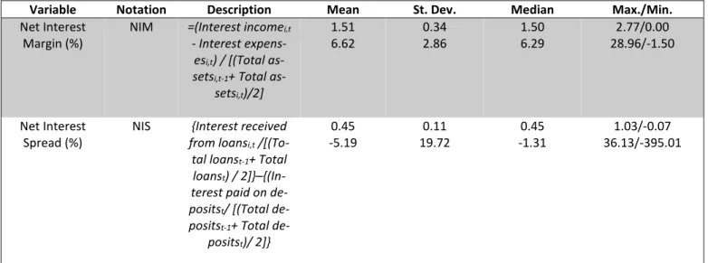
Table 2 Dependent Variables
The Dependent Variables for this study, which are the Net Interest Margins and the Net Interest Spreads are listed here, cov-ering their notations, descriptions and statistical details such as the means, standard deviations, medians, maximums and
min-imums.
Variable Notation Description Mean St. Dev. Median Max./Min.
Net Interest Margin (%)
NIM =(Interest incomei,t
- Interest expens-esi,t) / [(Total
as-setsi,t-1+ Total
as-setsi,t)/2] 1.51 6.62 0.34 2.86 1.50 6.29 2.77/0.00 28.96/-1.50 Net Interest Spread (%)
NIS {Interest received from loansi,t
/[(To-tal loanst-1+ Total
loanst) /
2]}–{(In-terest paid on de-positst/ [(Total
de-positst-1+ Total
de-positst)/ 2]} 0.45 -5.19 0.11 19.72 0.45 -1.31 1.03/-0.07 36.13/-395.01
25 Figure 1
Net Interest Margins & Net Interest Spreads
Here the standard deviations and coefficients of variation of Net Interest Margins & Net Interest Spreads (2005-2014) for the entire commercial banking sectors in Russia and Japan are illustrated. The coefficients of variation serve as the interpretation of relative dispersion. The standard deviation is hereby measured in terms of its proportion to the mean. The standard
devia-tions and coefficients of variadevia-tions are both presented as percentages
0 1 2 3 4 5 6 7 8 9 2005 2006 2007 2008 2009 2010 2011 2012 2013 2014
Net Interest Margin: Standard Deviation
Russia Japan 0 20 40 60 80 100 120 140 160 2005 2006 2007 2008 2009 2010 2011 2012 2013 2014
Net Interest Margin: Coefficient of Variation Russia Japan 0 0.2 0.4 0.6 0.8 1 1.2 2005 2006 2007 2008 2009 2010 2011 2012 2013 2014
Net Interest Spread: Standard Deviation
Russia Japan 0 500 1000 1500 2000 2500 3000 2005 2006 2007 2008 2009 2010 2011 2012 2013 2014
Net Interest Spread: Coefficient of Variation
26
3.3 Independent Variables
Table 3
Bank-Specific Variables
Among the independent variables, more precisely the bank-specific variables` notations and descriptions are included in this table, together with their statistical details such as the means, standard deviations, medians, maximums and minimums.
Variable Notation Description Mean St. Dev. Median Max/Min.
Size TA Total Assets 70,837,700 1,237,579 213,110,533 9,080,927 24,798,134 90,645 2,005,370.659/996,740 267,910,612/440 Profitability ROAA Return on
Av-erage Assets (%) 0.15 1.53 0.67 3.26 0.22 1.17 6.17/-9.70 55.73/-109.12 Liquidity Risk LIQ Liquid Assets
to Short-Term Liabilities (%) 7.50 66.27 7.99 58.34 5.66 54.41 91.73/1.49 967.98/2.22 Substitution Ef-fect
SUB Total Non-In-terest Income to Total Assets (%) 0.27 17.90 0.26 22.31 0.26 11.06 1.81 / -2.65 339.57/-11.32
Cost Efficiency CTP Cost-to-In-come Ratio (%) 70.83 81.92 32.45 21.80 69.65 88.80 784.62/38.26 759.41/8.86 Risk Aversion &
Capitalization
EQT Equity to Total Assets Ratio (%) 5.20 19.47 2.99 13.65 5.08 15.02 84.95/-14.43 99.83/-64.54
*Liquid Assets to Short-Term Liabilities along with Total Non-Interest Income to Total Assets: Own calculations by usage of Bankscope data
Table 4
Market-Specific Variables
Among the independent variables, more precisely the market-specific variables` notations and descriptions are included in this table, together with their statistical details such as the means, standard deviations, medians, maximums and minimums
Variable Notation Description Mean St. Dev. Median Max./Min.
Herfindahl-Hirschman
In-dex
HHD Market Concen-tration for
De-posits 3.94 1.65 28.24 23.90 0.09 0.00 505.37/0.00 632.76/0.00 Herfindahl-Hirschman In-dex HHL Market Concen-tration for Loans 6.04 1.65 37.46 27.51 0.12 0.00 400.21/0.00 724.37/0.00
*Herfindahl-Hirschman Indexes for Deposits and Loans: Own calculations by usage of Bankscope data Table 5
Microeconomic-Specific Variables
Among the independent variables, more precisely the microeconomic-specific variables` notations and descriptions are in-cluded in this table, together with their statistical details such as the means, standard deviations, medians, maximums and
27
Variable Notation Description Mean St. Dev. Median Max./Min.
Private Sector Debt
PSD Private Sector Debt to GDP – takes into ac-count only the debt of
non-fi-nancials and households, but not of fi-nancial corpo-rations 170.33 55.81 4.00 11.28 169.40 55.93 179.63/166.20 70.83/33.16 Government Debt GD Government Debt to GDP 212.89 11.72 24.98 2.47 213.10 11.49 245.05/183.01 15.91/7.98
*Private Sector Debt: Own calculations by usage of Russian Central Bank (CBR), Federal Reserve Bank of St. Louis and World Bank data
Table 6
Macroeconomic-Specific Variables
Among the independent variables, more precisely the macroeconomic-specific variables` notations and descriptions are in-cluded in this table, together with their statistical details such as the means, standard deviations, medians, maximums and
minimums.
Variable Notation Description Mean St. Dev. Median Max./Min.
Economic Growth GDP Real GDP per capita growth 0.66 3.33 2.68 4.98 1.46 4.32 4.63/-5.52 8.72/-7.85
Inflation INFL Inflation 0.21
9.21 1.14 2.86 0.01 8.72 2.74/-1.35 14.11/ 5.07 3.4 Expected Impacts Table 7 Expected Impacts
The independent variables are listed in the table with the expected impacts they are likely to have on the net interest margins and the net interest spread. Moreover, the number of observations are indicated. The first figure shows the number of
obser-vations for Japan, whereas the second one stands for Russia. The third number is the total sum of obserobser-vations sorted out in the dataset
Variable Expected Impact NIM Expected Impact NIS Observations
Net Interest Margin - - 1,106/4,674=5,780
Net Interest Spread - - 1,110/4,870=5,980
Size Positive/Negative Positive/Negative 1,106/4,716=5,822
Profitability Negative Negative 1,106/4,705=5,811
Liquidity Risk Negative Negative 1,105/4,583=5,688
Substitution Effect Negative Negative 1,110/4,850=5,960
Bank Efficiency Positive Positive 1,103/4,711=5,814
Risk Aversion & Capitalization Positive Positive 1,106/4,648=5,754
Herfindahl-Hirschman Index (D) Positive Positive 1,108/4,687=5,795
Herfindahl-Hirschman Index (L) Positive Positive 1,108/4,736=5,844
28
Government Debt Positive Positive 10/10=20
Economic Growth Positive Positive 10/10=20
Inflation Positive Positive 10/10=20
3.5 Methodology
The five core components of my methodology part are the following:
Correlation Matrix: Before running the panel fixed effects regression (OLS), I will create a correlation matrix in order to check whether there is a significant positive correlation between independent variables and get an insight into possible multi-collinearity. Those variables correlating strongly with each other will be taken out from the panel regression, mainly those having significant correlations at the 1% and 5% levels. If I have two variables explaining the same aspect in a regression they ought to be removed. High correlations among the variables produce “unreliable and unstable estimates of regression coefficients”49.
The Variance Inflation Factor (VIF) serves a support tool to decide on which one of the significantly correlated variables should be dropped. The VIF is computed for each predictor by conducting a linear regression of that predictor on all the other predictors, and afterwards receiving the R2 from that regression. The VIF is complemented by 1/(1-R2). It is an estimation of how much the variance of a coefficient is inflated due to linear dependence with other variables. A VIF of 1.7 tells that the variance - being the square of the standard error of a particular coefficient - is 70% larger than it would be if that predictor was entirely uncorrelated with all the other predictors. Bank-specific, market-specific, micro- and macroeco-nomic-specific variables will be all considered together for possible significantly positive correlations. Augmented Dickey-Fuller Test: This test serves to make sure the order of integration and the order of differencing necessary to make each time series stationary. This test is relevant when you have small N (few banks) observed over many years, meaning with a large T. However, since I have an annual dataset for 10 years with up to 139 banks in the full dataset for the Japanese and 827 banks for the Russian commercial banking sector, I opted to drop the testing of unit roots within the framework of the Aug-mented Dickey-Fuller Test. On the other hand, it is consensually considered that GDP growth (though not GDP levels!), inflation and other growth rates included in this study are stationary, so this justifies not to be particularly concerned with the issue.
29
Autocorrelation: As the EViews package does not automatically use t-statistics (or z-statistics) with auto-correlation - consistent standard errors, the standard errors will underestimate the actual estimation uncer-tainty, so that I would find a larger number of significant regressors than there is in reality. Thus, I imple-mented the White Period method, which handles clustering by cross-section. This method assumes that the errors for a cross-section are heteroskedastic and serially correlated. The resulting t-statistics are thus autocorrelation and heteroscedasticity-consistent.
OLS panel regression: This dated panel regression will define which the significant driving factors of Japanese and Russian net interest margins and spreads are. Moreover, I will look into fixed and random effect models and explain which one is more appropriate for my study.
NIMi,t = β0 + β1*TAi,t + β2*ROAAi,t + β3*LIQi,t + β4*SUBi,t + β5*CTPi,t + β6*EQTi,t + β7*HHDt + β8*HHLt + β9*PSDt + β10*GDt + β11*GDPt + β12*INFLt + β13D + εi,t
NISi,t = β0 + β1*TAi,t + β2*ROAAi,t + β3*LIQi,t + β4*SUBi,t + β5*CTPi,t + β6*EQTi,t + β7*HHDt +β8*HHLt + β9*PSDt + β10*GDt + β11*GDPt + β12*INFLt + β13D + εi,t
where i represents the individual bank, t equals the respective year, αi the fixed effects intercept and εit the
i.i.d. error term. To prevent direct effects of the 1998 Asian financial crisis and the Internet bubble in 2001, I concentrate on the sample period of 2005 to 2014, which helps me to direct my attention to the period before and after the 2008/09 crisis. The majority of the panel data models are estimated by the use of either random effects or fixed effects assumptions. Marno Verbeek’s book “A Guide to Modern Econo-metrics”50 supports me to identify the model, which is more suitable to my study. A fixed effects model
is a linear model in which intercept terms vary over individual commercial banks, but not over time. More specifically, the model can be laid out as: yit= αi+ x ́itβ+ εit, εit ∼ I.I.D (0,σ2ε) where yit stands for the
dependent variable for commercial bank i at time t, αi consider the characteristics that are one of a kind to
commercial bank i and do not alter over time, x ́it is a vector of explanatory variables and εit refers to the
disturbance term. This equation can also be put within the framework of a normal regression by including a dummy variable for each commercial bank i in the model as: yit = ∑𝑁𝑗=1 =αjdij+ x ́itβ+ εit, where dij = 1
if i = j and 0 elsewhere. The parameters α1, α2,...,αN and β can be estimated by OLS and the estimator for
β in that case is generally denoted as Least Squares Dummy Variables (LSDV) estimator. To reduce the
30
inconvenience of working with numerous dummy variables, the data can be changed into a much easier form through the implementation of a procedure named “within transformation”.
Hence, the OLS estimator of β of the moderated model is generally called fixed effects estimator. On the flipside, a random effects model presumes that all the sample observations are taken from the same distri-bution with the same mean and variance. To put differently, it assumes that αi’s are random factors that
are identically and independently distributed over every bank individually. This model can be shown in the following simple form: yit = μ+ x ́itβ+ αi+ εit, εit ∼ I.I.D (0,σ2ε); αi∼I.I.D (0,σ2α), where μ is the intercept term, αi is the bank specific component of the error term, which does not change over time and εit is the
time-variant component. This model anticipates that as long as αi and εit are mutually independent and
independent of xjs (for all j and s), the OLS estimator is non-biased and proves to function under a high
degree of consistency. If the assumptions of random effects model are true, I can ensure with strong con-fidence that it is more efficient than a fixed effects model, thus it should be favored. In contrast, due to the dataset comprising recurrent observations over the same commercial banks, it may not make sense to anticipate that different observations are independent from each other. For example, net interest margins and spreads of individual commercial banks may be under the influence of unobservable bank character-istics that modify themselves sparsely over time. For that reason, a non-compliance of the independently and identically distributed error terms assumption may cause the computed standard errors for the OLS estimator in random effects model to be plainly wrong. Considering these facts, a fixed effects model has a heightened potential to be more efficient than a random effects model. The implementation of the un-balanced panel regression gives enough sample observations to create statistical conclusions. A dummy variable (D) is implemented to consider the time effects, where dummy D = 1 if post-crisis period (2005-2008), and otherwise dummy = 0 if pre-crisis period (2009-2014).
Robustness Tests: Here I excluded banks with major foreign and state ownership structure. Furthermore, I would like to replace the following variables in order to see the effects they have on spreads and margins: Exclude banks with foreign ownership, then exclude state banks. The third step involves including
both foreign banks & state banks
Replacement of GDP per capita growth with population growth Replacement of inflation with real money supply growth M2