Evaluation of a regional air quality model using satellite column NO<sub>2</sub>: treatment of observation errors and model boundary conditions and emissions

(1)

ACPD

14, 21749–21784, 2014

Evaluation of a regional air quality model using satellite

column NO2

R. Pope et al.

Title Page

Abstract Introduction

Conclusions References

Tables Figures

◭ ◮

Back Close

Full Screen / Esc

Printer-friendly Version Interactive Discussion

Discussion

P

a

per

|

Discus

sion

P

a

per

|

Discussion

P

a

per

|

Discussion

P

a

per

|

Atmos. Chem. Phys. Discuss., 14, 21749–21784, 2014 www.atmos-chem-phys-discuss.net/14/21749/2014/ doi:10.5194/acpd-14-21749-2014

This discussion paper is/has been under review for the journal Atmospheric Chemistry and Physics (ACP). Please refer to the corresponding final paper in ACP if available.

Evaluation of a regional air quality model

using satellite column NO

₂

: treatment of

observation errors and model boundary

conditions and emissions

R. J. Pope1, M. P. Chipperfield1, N. H. Savage2, C. Ordóñez2, L. S. Neal2, L. A. Lee1, S. S. Dhomse1, and N. A. D. Richards1

1

School of Earth and Environment, University of Leeds LS2 9JT, Leeds, UK

2

Met Oﬃ_{ce, Exeter, UK}

Received: 1 July 2014 – Accepted: 13 July 2014 – Published: 26 August 2014 Correspondence to: R. Pope (eerjp@leeds.ac.uk)

(2)

ACPD

14, 21749–21784, 2014

column NO2

R. Pope et al.

Title Page

Tables Figures

◭ ◮

Back Close

Full Screen / Esc

Discussion

P

a

per

|

Discus

sion

P

a

per

|

Discussion

P

a

per

|

Discussion

P

a

per

|

Abstract

We compare tropospheric column NO2 between the UK Met Oﬃce operational Air

Quality in the Unified Model (AQUM) and satellite observations from the Ozone Moni-toring Instrument (OMI) for 2006. Column NO₂retrievals from satellite instruments are prone to large uncertainty from random, systematic and smoothing errors. We present 5

an algorithm to reduce the random error of time-averaged observations, once smooth-ing errors have been removed with application of satellite averagsmooth-ing kernels to the model data. This reduces the total error in seasonal mean columns by 30–90 %, which allows critical evaluation of the model. The standard AQUM configuration evaluated here uses chemical lateral boundary conditions (LBCs) from the GEMS (Global and 10

regional Earth-system Monitoring using Satellite and in-situ data) reanalysis. In sum-mer the standard AQUM overestimates column NO2 in northern England and

Scot-land, but underestimates it over continental Europe. In winter, the model overestimates column NO2 across the domain. We show that missing heterogeneous hydrolysis of

N2O5 in AQUM is a significant sink of column NO2 and that the introduction of this

15

process corrects some of the winter biases. The sensitivity of AQUM summer column NO2 to diﬀerent chemical LBCs and NOx emissions datasets are investigated. Using

Monitoring Atmospheric Composition and Climate (MACC) LBCs increases AQUM O3

concentrations compared with the default GEMS LBCs. This enhances the NO_x-O₃ coupling leading to increased AQUM column NO2in both summer and winter

degrad-20

ing the comparisons with OMI. Sensitivity experiments suggest that the cause of the remaining northern England and Scotland summer column NO₂ overestimation is the representation of point source (power station) emissions in the model.

1 Introduction

Air quality has a major influence on the UK both socially and economically. It can result 25

(3)

ACPD

14, 21749–21784, 2014

column NO2

R. Pope et al.

Title Page

Tables Figures

◭ ◮

Back Close

Full Screen / Esc

Discussion

P

a

per

|

Discus

sion

P

a

per

|

Discussion

P

a

per

|

Discussion

P

a

per

|

expectancy of 7–8 months (HoC, 2010). Air pollution health eﬀ_{ects include lung}

dis-ease and cancer, cardiovascular problems, asthma and eye irritation (WHO, 2011). In 2005 poor UK air quality cost £ (€_{) 8.5 (10.7)–20.2 (25.5) billion and between 2007–}

2008 there were 74 000 asthma-related hospital admissions. Overall, these air quality-asthma incidents cost society £ (€_{) 2.3 (2.9) billion (HoC, 2010). Poor air quality}

asso-5

ciated with ozone concentrations over 40 ppbv can also significantly reduce crop yields e.g. Hollaway et al. (2012).

Therefore, regional models have been developed to predict hazardous levels of air pollution to help inform the public and to allow local authorities to take action to re-duce/accommodate the respective health risks/eﬀ_{ects. Air quality models have mainly}

10

been evaluated against surface observations, e.g. Savage et al. (2013). However, re-cently such models have also been compared with satellite observations, taking ad-vantage of the better spatial coverage despite the potentially large error of individual observations. In the past NO₂satellite data has been compared mainly with global at-mospheric chemistry models (e.g. Velders et al., 2001; Lauer et al., 2002; Van Noije 15

et al., 2006). However, more recently, other studies have used satellite data to evaluate models on a regional scale. Savage et al. (2008) investigated European tropospheric column NO2 interannual variability (IAV), 1996–2000, by comparing GOME with the

TOMCAT chemical transport model (CTM) (Monks et al., 2012). The best comparisons were found in the JFM and AMJ seasons, especially over western Europe. They also 20

found that synoptic meteorology had more influence on NO2 IAV than NOx emissions

did.

Huijnen et al. (2010) compared Ozone Monitoring Instrument (OMI) tropospheric column NO2 against a European global-regional air quality model ensemble median

for 2008–2009. The ensemble compared better with the OMI data than any one model, 25

with good agreement over the urban hotspots. Overall, the spread in the models was greatest in the summer (with deviations from the mean OMI tropospheric column in the range 40–62 %), due to the more active NOx chemistry in this season and the

(4)

ACPD

14, 21749–21784, 2014

column NO2

R. Pope et al.

Title Page

Tables Figures

◭ ◮

Back Close

Full Screen / Esc

Discussion

P

a

per

|

Discus

sion

P

a

per

|

Discussion

P

a

per

|

Discussion

P

a

per

|

winter (20–34 %). Several of the regional models successfully detected the shipping lanes seen by OMI.

Han et al. (2011) investigated tropospheric column NO2 over the Korean Peninsula

through comparisons between OMI data and the Community Multi-scale Air Quality Model (CMAQ) (Foley et al., 2010). In summer North and South Korea had similar col-5

umn NO2from both model and observations. However, in winter South Korea, a more

developed nation with greater infrastructure, had significantly greater NO₂ concentra-tions than North Korea. Overall, CMAQ overestimated OMI NO2concentrations by

fac-tors of 1.38–1.87 and 1.55–7.46 over South and North Korea, respectively.

Other studies investigating regional tropospheric column NO₂ through model sim-10

ulations and satellite observations include Blond et al. (2007), Boersma et al. (2009) and Curier et al. (2014). Blond et al. (2007) compared CHIMERE 3-D CTM and SCIA-MACHY column NO2over western Europe with good agreement with winter and

sum-mer correlations of 0.79 and 0.82, respectively. Boersma et al. (2009) used the GEOS-Chem 3-D CTM to explain the seasonal cycle in SCIAMACHY and OMI column NO2

15

over Israeli cities, with larger photochemical loss of NO2 in summer than winter. And

Curier et al. (2014) used a synergistic of OMI and the LOTOS-EUROS 3-D CTM to evaluate NOxtrends finding negative trends of 5–6 % over western Europe.

The UK Met Oﬃ_{ce’s Air Quality in the Unified Model (AQUM) is used for short}

opera-tional chemical weather forecasts of UK air quality. Savage et al. (2013) performed the 20

first evaluation of the AQUM operational forecast for the period May 2010–April 2011 by using surface O3, NO2and particulate matter observations from the UK Automated

Urban and Rural Network (AURN) (DEFRA, 2012). Among other model-observation metrics they used the mean bias (MB), root mean square error (RMSE), modified nor-malised mean bias (MNMB) and the Fractional Gross Error (FGE) (Seigneur et al., 25

2000). See the Appendix for the definition of these metrics.

Savage et al. (2013) found that AQUM overestimated O3 by 8.38 µg m− 3

(MNMB=_{0.12), with a positive bias at urban sites but no systematic bias at rural sites.}

(5)

ACPD

14, 21749–21784, 2014

column NO2

R. Pope et al.

Title Page

Tables Figures

◭ ◮

Back Close

Full Screen / Esc

Discussion

P

a

per

|

Discus

sion

P

a

per

|

Discussion

P

a

per

|

Discussion

P

a

per

|

a bias of−6.10 µg m−3, correlation of 0.57 and MNMB of −0.26. At urban sites there

was a large negative bias while rural sites had marginal positive biases. The coarse resolution of AQUM (12 km) led to an underestimation at urban sites because the model NOx emissions are instantaneously spread over the entire grid box. The

par-ticulate matter (PM10) prediction skill was lower with a correlation and bias of 0.52 and

5

−9.17 µg m−3, respectively.

The aim of this paper is to evaluate AQUM using satellite atmospheric trace gas observations. The Met Oﬃ_{ce has previously compared the skill of AQUM only against}

AURN surface measurements, which in the case of NO₂ are not specific and include contributions from other oxidised nitrogen compounds (see Savage et al. (2013), and 10

references therein). Therefore, for better spatial model-observation comparisons and to minimise the eﬀ_{ect of measurement interferences, we use satellite observations}

over the UK. We focus on tropospheric column NO2 data from OMI for the summer

(April–September) and winter (January–March, October–December) periods of 2006. Section 2 describes the OMI satellite data used and gives a detailed account of our 15

error analysis which determines how we can use satellite data to test AQUM. Sec-tion 3 describes AQUM and the model experiments performed. Results from the model-observations comparisons are given in Sect. 4. Section 5 presents our conclusions.

2 Satellite data

OMI is aboard NASA’s EOS-Aura satellite and has an approximate London daytime 20

overpass at 13:00 LT. It is a nadir-viewing instrument with a pixel size of 312 km2 and 3240 km2 along track and across track, respectively (Boersma et al., 2008). We have taken the DOMINO tropospheric column NO₂ product, version 2.0, from the TEMIS (Tropospheric Emissions Monitoring Internet Service) website, http://www.temis.nl/ airpollution/no2.html (Boersma et al., 2011b, a). We have binned NO2 swath data

25

from 1 January to 31 December 2006 onto a daily 13:00 LT 0.25◦

×0.25◦ grid between

(6)

re-ACPD

14, 21749–21784, 2014

column NO2

R. Pope et al.

Title Page

Tables Figures

◭ ◮

Back Close

Full Screen / Esc

Discussion

P

a

per

|

Discus

sion

P

a

per

|

Discussion

P

a

per

|

Discussion

P

a

per

|

trievals/pixels with geometric cloud cover greater than 20 % and poor quality data flags (flag=₋_{1) were removed. The product uses the algorithm of Braak (2010) to identify}

OMI pixels aﬀ_{ected by row anomalies and sets the data flags to}₋_{1. We also filter these}

out in this study. Even though OMI has an approximate 13:00 LT London overpass, we used all OMI retrievals in the domain between 11:00 and 15:00 LT to get more exten-5

sive spatial coverage. Several studies have validated OMI column NO2against surface

and aircraft measurements of tropospheric column NO₂. Irie et al. (2008) compared OMI and with ground based MAX-DOAS retrievals in the Mount Tai Experiment (2006). They found the standard OMI product (version 3) overestimated the MAX-DOAS mea-surements by approximately 1.6_×1015molecules cm−2 _{(20 %), but within the OMI}

un-10

certainty limits. Boersma et al. (2008) compared the near real time (NRT) OMI product (version 0.8) with aircraft measurements in the INTEX-B campaign. Overall, they found a good correlation (0.69) between OMI and the aircraft column NO2, with no significant

biases. Therefore, we have confidence in the OMI column NO₂and use it for evaluation of our model.

15

2.1 Satellite averaging kernels

Eskes and Boersma (2003) define the averaging kernel (AK) to be a relationship be-tween the retrieved quantities and the true distribution of the tracer. In other words, the satellite instrument’s capability to retrieve a quantity is a function of altitude. For instance, the instrument may be more or less sensitive retrieving a chemical species 20

near the boundary layer than in the stratosphere. Therefore, since satellite retrievals and model vertical profiles are not directly comparable, the AK (or weighting function) is applied to the model data, so the sensitivity of the satellite is accounted for in the comparisons. The AK comes in diﬀ_{erent forms for di}ﬀ_{erent retrieval methods. For the}

Diﬀ_{erential Optical Absorption Spectroscopy (DOAS) method, the AK is in the form of}

25

(7)

ACPD

14, 21749–21784, 2014

column NO2

R. Pope et al.

Title Page

Tables Figures

◭ ◮

Back Close

Full Screen / Esc

Discussion

P

a

per

|

Discus

sion

P

a

per

|

Discussion

P

a

per

|

Discussion

P

a

per

|

The OMI retrievals use the DOAS technique and the AK is a column vector. Following Huijnen et al. (2010) and the OMI documentation (Boersma et al., 2011a), the AKs are applied to the model as:

y=_A_·_x ₍₁₎

wherey is the total column,Ais the AK and x is the vertical model profile. However, 5

here the tropospheric column is needed:

ytrop=Atrop·xtrop (2)

whereAtropis:

Atrop=A·

AMF

AMF_trop (3)

AMF is the atmospheric air mass factor and AMFtrop is the tropospheric air mass

10

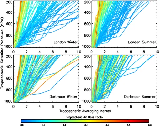
factor. For the OMI product, Huijnen et al. (2010) state the AK tends to be lower than 1 in the lower troposphere (e.g. 0.2–0.7 up to 800 hPa) and greater than 1 in the mid-upper troposphere. Therefore, the OMI AKs reduce model NO2 subcolumns in the

lower troposphere and increase them in the mid-upper troposphere (Huijnen et al., 2010). Figure 1 shows example tropospheric AKs for summer and winter profiles over 15

London (urban – higher column NO2) and Dartmoor (rural area in southwest England

– lower column NO₂), which have been coloured by their respective tropospheric AMF. In the lower troposphere for both seasons and locations the tropospheric AKs range around 0–1. However, in the mid-upper troposphere, the London tropospheric AKs tend to be greater than Dartmoor in both seasons. London tropospheric AKs are most pro-20

(8)

ACPD

14, 21749–21784, 2014

column NO2

R. Pope et al.

Title Page

Tables Figures

◭ ◮

Back Close

Full Screen / Esc

Discussion

P

a

per

|

Discus

sion

P

a

per

|

Discussion

P

a

per

|

Discussion

P

a

per

|

NO₂ is within the lower layers of the London boundary layer; also small tropospheric AKs there), from Eq. (3), as the full atmospheric AKs naturally increase with altitude, the tropospheric AMFs will return larger tropospheric AKs. Also, in winter over Lon-don, the shallower boundary layer with trap larger winter emissions of NO₂ closer to the surface. Therefore, the tropospheric AMF will be smaller and the winter mid-upper 5

tropospheric AKs will be larger as seen in Fig. 1. Over Dartmoor, the AKs show less seasonal variation and the majority range around 1–6 for both summer and winter. This is also seen in the tropospheric AMF, which ranges between approximately 0–6, but has no clear pattern in the Dartmoor tropospheric AKs, in both seasons.

2.2 Di_fferential optical absorption spectroscopy NO2retrieval error

10

The DOAS retrievals are subject to random, systematic and smoothing errors in the retrieval process. Random (quasi-systematic) errors include fitting errors, cloud errors, instrument noise and signal corruption. Systematic errors include absorption cross-sections, surface albedo and stratospheric correction uncertainties. Finally, smoothing errors include biases in the a priori profiles and sensitivity of the satellite when record-15

ing the slant column through the atmosphere. If multiple retrievals are averaged to-gether, as in this study, the random errors will partially cancel leading to the random error being reduced by a factor of √1

N (whereN is the number of retrievals).

In contrast, systematic errors are unaﬀ_{ected by cancelling through averaging. In the}

following section we investigate the diﬀ_{erent error components of the satellite retrievals}

20

and derive an expression for the error in the averaged retrievals. This methodology should give smaller errors which are more representative of the time-averaged retrieval error and so allow a stricter test of the model. Boersma et al. (2004) describe the error in the DOAS NO2retrievals as:

σ_trop2 = σtotal

AMFtrop

!2

+ σstrat

AMFtrop

!2 +





(Xtotal−Xstrat)σAMF_trop

AMF2_trop





2

(9)

ACPD

14, 21749–21784, 2014

column NO2

R. Pope et al.

Title Page

Tables Figures

◭ ◮

Back Close

Full Screen / Esc

Discussion

P

a

per

|

Discus

sion

P

a

per

|

Discussion

P

a

per

|

Discussion

P

a

per

|

whereσtrop,σstratandσtotalare the uncertainties in the tropospheric, stratospheric and

total slant columns, respectively. AMF_tropis the tropospheric air mass factor,σ_AMF

trop is the error in the tropospheric air mass factor,Xtotalis the total slant column andXstratis

the stratospheric slant column.

σtotal is made up of both random and systematic error, where the random error

5

component can be reduced by √1

N. We assume that the systematic and random er-rors can be combined in quadrature. In Eq. (6) there are two terms for σtotal; σtotal_ran

andσtotal_sys, which are the random and systematic error components of the total slant

column, respectively. Boersma et al. (2004) state that σtotal_sys can be expressed as

σtotal_sys=0.03Xtotal. We treat σstrat here as systematic as both the OMI standard and

10

DOMINO products estimate the stratospheric slant column using TM4 chemistry-transport model simulations and data assimilation (Dirksen et al., 2011). According to the DOMINO OMI product documentation (which references Boersma et al., 2004, 2007; Dirksen et al., 2011), the error in the stratospheric slant column is estimated to be 0.25×1015molecules cm−2in all cases.

15

Boersma et al. (2004) state that the tropospheric column is calculated as:

Ntrop=

X_total₋X_strat

AMFtrop

(5)

whereNtrop is the vertical tropospheric column and can be substituted, including the

σtotalandσstrat estimates, into Eq. (4). This leads to:

σ_trop2 = σtotalran

AMF_trop

!2

+ 0.03Xtotal

AMF_trop

!2

+ 0.25×10

15

AMF_trop

!2 +

NtropσAMF_trop

AMF_trop

!2

(6) 20

σtropis reduced in the model-satellite comparisons when the AK is applied to the model

data. Therefore, the error product,σtrop_ak, from the OMI retrieval files with the smoothing

(10)

ACPD

14, 21749–21784, 2014

column NO2

R. Pope et al.

Title Page Abstract Introduction Conclusions References Tables Figures ◭ ◮ ◭ ◮ Back Close

Full Screen / Esc

Printer-friendly Version Interactive Discussion Discussion P a per | Discus sion P a per | Discussion P a per | Discussion P a per |

Boersma et al. (2007) suggest that the uncertainty in the tropospheric AMF is be-tween 10–40 %. Therefore, we take the conservative estimate ofσAMF_trop=0.4·AMFtrop.

This leads to the new retrieval error approximation of:

σ_trop2

ak

= σtotalran

AMF_trop

!2

+ 0.03Xtotal

AMF_trop

!2

+ 0.25×10

15

AMF_trop

!2

+ _0.4_N

trop

2

(7)

All of these terms are known apart from σtotal_ran. We can rearrange to calculate this

5

based on other variables provided in the OMI product files. This leads to:

σtotal_ran

AMFtrop

!2 =_σ2

trop_ak− 0.4Ntrop

2 −

0.03Xtotal

AMFtrop

!2

− 0.25×10

15

AMFtrop

!2

(8)

In the rare case that the left hand side is negative, the random error component cannot be found as it would be complex, so the random error component is then set to 50 % (H. Eskes, personal communication, 2012). Now, rearranging forσ_total

ran, and 10

assuming the left hand side is positive, Eq. (8) becomes:

σtotal_ran= AMFtrop

v u u t

σ_trop2

ak

− 0.4Ntrop

2 −

0.03Xtotal

AMFtrop

!2

− 0.25×10

15

AMFtrop

!2

(9)

This quantity was calculated for each retrieval in each grid square and then the new seasonal retrieval error was calculated taking the reduced random component into account:

15

σtrop_ak=

v u u u t  

σtotal_ran

√

NAMF_trop

  2 +  

0.03Xtotal

AMF_trop   2 +  

0.25×1015

AMF_trop





2

+_0.4_N_trop2 ₍₁₀₎

(11)

ACPD

14, 21749–21784, 2014

column NO2

R. Pope et al.

Title Page

Tables Figures

◭ ◮

Back Close

Full Screen / Esc

Discussion

P

a

per

|

Discus

sion

P

a

per

|

Discussion

P

a

per

|

Discussion

P

a

per

|

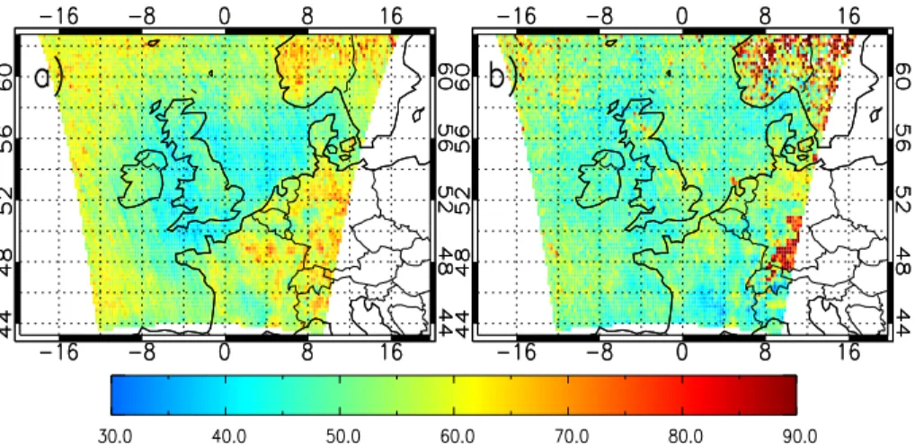
Figure 2 shows how averaging, by decreasing the random error component, reduces the seasonal satellite tropospheric column error as calculated by our algorithm. The figure compares the simple mean of the total satellite column NO2error (calculated for

each pixel) with our new method which reduces the estimated random error component by one over the square root of the number of observations. The reduction in the satellite 5

column error is then presented as a percentage of the original satellite column seasonal mean error. In both summer and winter, the seasonal mean column error is reduced to 30–90 % across the domain, therefore making the OMI data much more useful for model evaluation. Only for a few retrievals over Scandinavia, does this methodology of reducing the random error component increase the overall column error (not shown 10

here).

3 Air quality in the unified model (AQUM)

3.1 Model setup

The AQUM domain covers the UK and part of continental Europe on a rotated grid be-tween approximately 45–60◦_{N and 12}◦_W–12◦_{E. The model has a horizontal resolution}

15

of 0.11◦

×0.11◦ with 38 vertical levels between the surface and 39 km. The model has

a coupled, online tropospheric chemistry scheme using the UK Chemistry and Aerosols (UKCA) subroutines. The chemistry scheme (Regional Air Quality, RAQ) includes 40 tracers, 23 photolysis reactions and 115 gas-phase reactions (Savage et al., 2013) including the reaction of nitrate radical with formaldehyde, ethene, ethane, propane, 20

n-butane, acetaldehyde and isoprene. The standard model setup does not include any heterogeneous chemistry. A complete chemical mechanism is included in the online supplement to Savage et al. (2013).

The model uses the Coupled Large-scale Aerosol Simulator for Studies In Climate (CLASSIC) aerosol scheme. This is a bulk aerosol scheme with the aerosols treated 25

(12)

ammo-ACPD

14, 21749–21784, 2014

column NO2

R. Pope et al.

Title Page

Tables Figures

◭ ◮

Back Close

Full Screen / Esc

Discussion

P

a

per

|

Discus

sion

P

a

per

|

Discussion

P

a

per

|

Discussion

P

a

per

|

nium sulphate, mineral dust, fossil fuel black carbon (FFBC), fossil fuel organic carbon (FFOC), biomass burning aerosols and ammonium nitrate. In addition, there is a di-agnostic aerosol scheme for sea salt and a fixed climatology of biogenic secondary organic aerosols (BSOA). For more details of the aerosol scheme see Bellouin et al. (2011). In common with most regional AQ forecast models in Europe, AQUM shows 5

a small negative bias for PM2.5and a larger negative bias for PM10. For full details of

the performance of the model for aerosols, NO₂and ozone see Savage et al. (2013). Meteorological initial conditions and lateral boundary conditions (LBCs) come from the Met Oﬃ_{ce’s operational global Unified Model (25 km}_×_{25 km) data. Initial}

chemi-cal conditions come from the previous day’s AQUM forecast and aerosol and chemistry 10

LBCs come from the ECMWF GEMS (Global and regional Earth-system Monitoring us-ing Satellite and in-situ data) reanalyses (Hollus-ingsworth et al., 2008). The GEMS fields, available at http://www.gmes-atmosphere.eu/, provide boundary fluxes for regional air quality models such as AQUM.

This configuration of AQUM uses emission datasets from the National Atmo-15

spheric Emissions Inventory (NAEI) (1 km×1 km) for the UK, ENTEC (5 km×5 km)

for the shipping lanes and European Monitoring and Evaluation Programme (EMEP) (50 km×50 km) for the rest of the model domain. Over the UK the NAEI NOx

emis-sions datasets are made up of two source types: area and point. Area sources include traﬃ_{c, light industry and urban emissions, while point sources are power stations,}

land-20

fill, incinerators and refineries. Typically, the point source emissions are 100 g s−1 _in

magnitude, while the area sources tend to be 10 g s−1_{. For most of the experiments}

we use 2007 instead of 2006 NO_x sources because the ENTEC shipping emissions (5 km×5 km resolution) are available for this year, while only the coarse EMEP

ship-ping emissions are available for the earlier years (Savage et al., 2013). The diﬀ_erence

25

between 2006 and 2007 point source emissions are negligible in altering the AQUM col-umn NO2(not shown). Therefore, we use the 2007 emissions datasets throughout this

(13)

ACPD

14, 21749–21784, 2014

column NO2

R. Pope et al.

Title Page

Tables Figures

◭ ◮

Back Close

Full Screen / Esc

Discussion

P

a

per

|

Discus

sion

P

a

per

|

Discussion

P

a

per

|

Discussion

P

a

per

|

parameterisation for soil NO_x emissions but given the large emissions from transport and industry, the soil NOxemissions are unlikely to be important in this region.

3.2 Sensitivity experiments

We performed one control and five sensitivity experiments to investigate the AQUM’s simulation of column NO₂. Two experiments used diﬀ_{erent LBCs, two experiments used}

5

modified point source emissions and two included heterogeneous chemistry. These are summarised in Table 1.

Simulation MACC investigates the sensitivity of AQUM column NO₂ to diﬀ_erent

chemical LBCs from the global Monitoring Atmospheric Composition and Climate (MACC) reanalyses, which is the follow-on project of GEMS (Inness et al., 2013). Sav-10

age et al. (2013) have undertaken a similar analysis of the MACC LBCs in AQUM. They showed that when compared with the AURN observations of O3, AQUM-MACC

performs well during the first quarter of 2006 and overestimates observations after-wards, while AQUM-GEMS has a negative bias during the first quarter of the year but compares well with observations afterwards.

15

We have performed additional runs to examine the impact of the point sources over the UK on NO₂ columns. The motivation behind Run E1 was to determine the impact of the NO_x point sources on the simulated column NO₂ budget, as we hypothesised that the AQUM’s representation of them was the cause of the AQUM–OMI column NO2

positive biases (see Sect. 4.1). Run E2 uses an idealised passive tracer from the point 20

sources with a lifetime of one day to examine if the tracer columns correlated with summer AQUM-OMI positive biases (see Sect. 4.3). Runs N2O5High and N2O5Low

investigate the impact of heterogeneous chemistry on NO2columns. Tropospheric NOx

(14)

ACPD

14, 21749–21784, 2014

column NO2

R. Pope et al.

Title Page

Tables Figures

◭ ◮

Back Close

Full Screen / Esc

Discussion

P

a

per

|

Discus

sion

P

a

per

|

Discussion

P

a

per

|

Discussion

P

a

per

|

to HNO₃is through two pathways:

NO₂+_OH+_M_→_HNO₃+_M _(R1)

NO₂+_O

3→NO3+O2 (R2)

NO3+NO2+M⇋N2O5+M (R3)

N2O5+H2O aerosol

−−−−−→2HNO3(aq) (R4)

5

The standard configuration of AQUM does not include any heterogeneous reac-tions such as the hydrolysis of N2O5on aerosol surfaces (see details of the chemistry

scheme in the Supplement of Savage et al., 2013). Previous global modelling studies have shown that this process can be a significant NOx sink at mid-latitudes in winter

(e.g. Tie et al., 2003; Macintyre and Evans, 2010). Following those analyses, we have 10

implemented this reaction, with ratek (s−1_{) calculated as:}

k=Aγω

4 (11)

whereA is the aerosol surface area (cm2cm−3_), _γ _{is the uptake coe}_ﬃ_{cient of N}

2O5

on aerosols (non-dimensional) and ω=_{100 [8RT}_/₍_π_M)]12 _{(cm s}−1_{) is the} root-mean-square molecular speed of N2O5 at temperature T (K), M is the molecular mass of

15

N₂O₅(kg mol−1_{) and}_R₌_{8.3145 J mol}−1_K−1_.

Macintyre and Evans (2010) investigated the sensitivity of N2O5 loss on aerosol by

using a range of uptake values (0.0, 10−6_{, 10}−4_{, 10}−3_{, 5}

×10−3, 10−2, 2×10−2, 0.1,

0.2, 0.5 and 1.0). They found that limited sensitivity occurs at low and high values of

γ. At low values, the uptake pathway is an insignificant route for NOx loss. At high

20

values, the loss of NO_x through heterogeneous removal of N₂O₅is limited by the rate of production of NO3, rather than the rate of heterogeneous uptake. However, in the

northern extra-tropics (including the AQUM domain), intermediate values ofγ (0.001– 0.02) show a significant loss of NOx. Therefore, we experiment withγ=0.001 and 0.02

(15)

ACPD

14, 21749–21784, 2014

column NO2

R. Pope et al.

Title Page

Tables Figures

◭ ◮

Back Close

Full Screen / Esc

Discussion

P

a

per

|

Discus

sion

P

a

per

|

Discussion

P

a

per

|

Discussion

P

a

per

|

aerosol surface area, A, includes the contribution of seven aerosol types present in CLASSIC: sea salt aerosol, ammonium nitrate, ammonium sulphate, biomass burn-ing aerosol, black carbon, fossil fuel organic carbon (FFOC) and biogenic secondary organic aerosol (BSOA). To account for hydroscopic growth of the aerosols, the formu-lation of Fitzgerald (1975) is used for growth above the deliquescence point for ammo-5

nium sulphate (RH=_{81 %), sea salt (RH}=_{75 %) and ammonium nitrate (RH}=_{61 %)}

up to 99.5 % RH. We apply a linear fit between the eﬄ_{orescence (RH}=_{30 % for}

sul-phate, 42 % for sea-salt and 30 % for nitrate) and deliquescence points. There is no hy-droscopic growth below the eﬄ_{orescence point. Look-up tables are used for the other}

aerosol types. Biomass burning and FFOC aerosol growth rates are taken from Magi 10

and Hobbs (2003), BSOA growth rates come from Varutbangkul et al. (2006) and black carbon is hydrophobic (no growth).

3.3 Statistical comparisons

For the AQUM-satellite comparisons the following model-observation statistics were used: Mean Bias (MB), Root Mean Square Error (RMSE) and the Fractional Gross 15

Error (FGE, bounded by the values 0 to 2). These statistics are described by Han et al. (2011) and Savage et al. (2013). Further details are given in the Appendix.

4 Results

4.1 Control run

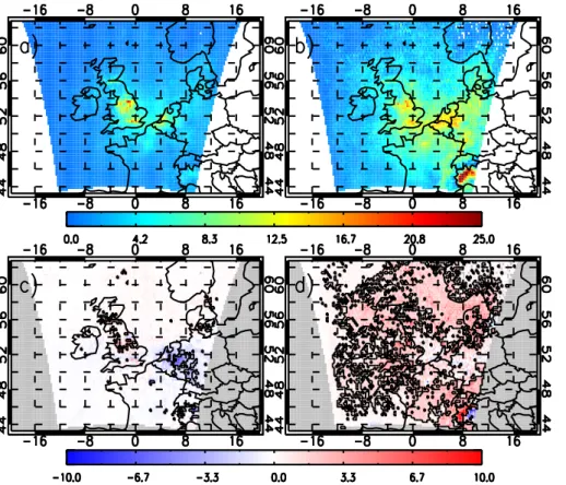
Figure 3 compares observed column NO2with the AQUM control Run C (with AKs

ap-20

(16)

ACPD

14, 21749–21784, 2014

column NO2

R. Pope et al.

Title Page

Tables Figures

◭ ◮

Back Close

Full Screen / Esc

Discussion

P

a

per

|

Discus

sion

P

a

per

|

Discussion

P

a

per

|

Discussion

P

a

per

|

The OMI peak column NO2of 16–20×10 15

molecules cm−2_{is over London. AQUM}

simulates similar London column NO2, but the model peak concentrations are over

northern England at over 20_×1015molecules cm−2_{. In winter, the background column}

NO2is elevated with a larger spatial extent ranging between 0–6×10 15

molecules cm−2

in both the AQUM and OMI fields. However, the elevated AQUM background state 5

has a larger coverage than that of OMI. Over the source regions, OMI column NO₂ peaks over London at 12–13_×1015molecules cm−2_{, with similar concentrations seen}

in AQUM. However, AQUM peak column NO2 are over northern England at 12–

16×1015molecules cm−2. Therefore, independent of season, AQUM overestimates

northern England column NO₂. Interestingly, the background column NO₂ is larger in 10

winter for both AQUM and OMI, but column NO2 is lower over the source regions in

winter than summer (Pope et al., 2014).

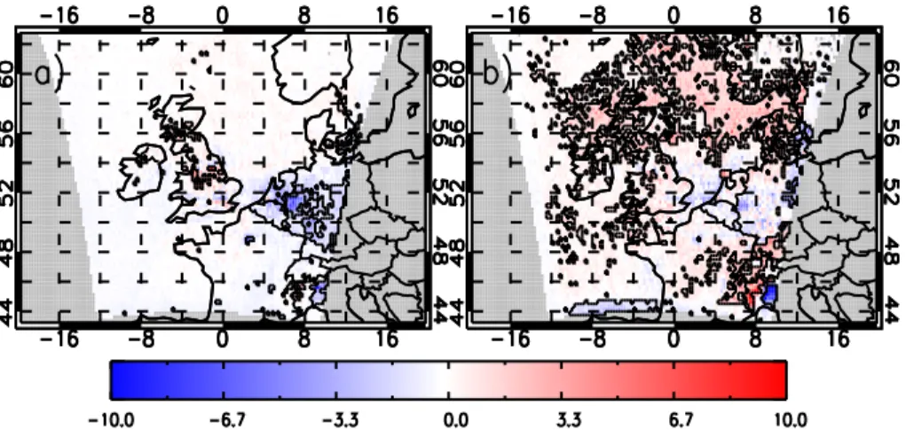
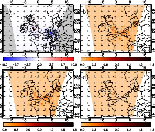
Figure 4 shows the MB between AQUM Run C and OMI. The black poly-goned regions show significant diﬀ_{erences, i.e. where the magnitude of the MB}

is greater than the satellite error. In summer, there are significant positive, 5– 15

10_×1015molecules cm−2_{, and negative,}

−10 to −1×1015molecules cm−2, biases in

northern England and the Benelux region, respectively. The negative biases are poten-tially linked to the coarser resolution EMEP NOx emissions datasets (50 km×50 km)

which average emissions over a larger grid square causing AQUM to simulate lower column NO2than seen by OMI. We hypothesise that the northern England biases are

20

linked to the point source (power station) NOxemissions from NAEI. This is further

dis-cussed in Sect. 4.3. In winter, AQUM overestimates OMI by 1–3×1015molecules cm−2

over the North Sea and Scotland, as the modelled winter background column NO₂is larger; this is further investigated in Sect. 4.4 by including an additional NOxsink in the

chemistry scheme of the model. The northern England biases seen in summer also 25

extend to winter, 3–5_×1015molecules cm−2_{, suggesting the northern England biases}

(17)

ACPD

14, 21749–21784, 2014

column NO2

R. Pope et al.

Title Page

Tables Figures

◭ ◮

Back Close

Full Screen / Esc

Discussion

P

a

per

|

Discus

sion

P

a

per

|

Discussion

P

a

per

|

Discussion

P

a

per

|

We also compared AQUM against surface observations of NO₂ from AURN, found at http://uk-air.defra.gov.uk/networks/network-info?view=_{aurn, and maintained by}

DE-FRA. This was to see if there was a consistent pattern in the biases in the model col-umn and surface NO₂. However, we find similar problems to Savage et al. (2013) where surface AQUM – observation comparisons have systematic negative biases at urban 5

sites. The coarse model resolution, compared to the observation point measurements (even with roadside and traﬃ_{c sites removed), results in significant model}

underesti-mation of NO2 at all urban regions. Therefore, it is diﬃcult to draw any conclusions

on the AQUM skill as the model grid-point data will struggle to reproduce the point measurement observations. Also the spatial coverage of the AURN data is very sparse 10

over the UK and AURN NO₂measurement interferences from molybdenum converters (Steinbacher et al., 2007) overestimate surface concentrations in rural sites. Therefore, satellite (pixel area) data are the primary observations used to evaluate AQUM in this paper.

4.2 Impact of lateral boundary conditions 15

Figure 5a and b shows results of the sensitivity run with the MACC boundary condi-tions (Run MACC) and can be compared with Fig. 3a and b. The MACC LBCs have a limited impact on summer column NO₂ with peak concentrations over London and Northern England between 15–20×1015molecules cm−2for both runs MACC and C.

However, in winter Run MACC increases column NO2from approximately 12×10 15

to 20

16_×1015molecules cm−2_{over the UK and Benelux region. When compared with OMI}

(Fig. 5a and b) the limited summer impact of the MACC LBCs results in biases which are similar to those in Fig. 4 from the control run, with biases over northern England, 5–10_×1015molecules cm−2_{, and continental Europe,}

−5 to−3×1015molecules cm−2.

In winter Run MACC has enhanced column NO₂ resulting in biases with OMI of be-25

tween 2–5×1015molecules cm−2across the whole domain, unlike Run C with GEMS

(18)

ACPD

14, 21749–21784, 2014

column NO2

R. Pope et al.

Title Page

Tables Figures

◭ ◮

Back Close

Full Screen / Esc

Discussion

P

a

per

|

Discus

sion

P

a

per

|

Discussion

P

a

per

|

Discussion

P

a

per

|

Valley), 5×1015molecules cm−2, suggesting that AQUM overestimates NO2in the

re-gion, at the OMI overpass time, independent of season or LBCs. Therefore, the GEMs LBCs appear to give better AQUM column NO₂forecast skill than MACC does, which is consistent with the findings of Savage et al. (2013) for the comparisons with surface ozone.

5

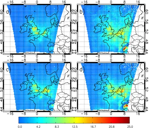
4.3 AQUM NOxemissions sensitivity experiments

We hypothesise that significant summer Run C–OMI positive biases in northern Eng-land and ScotEng-land (Fig. 4) are caused by the AQUM’s representation of point source (mainly power station) NOx emissions. Therefore, to better understand these biases,

we investigate sensitivity experiments of NO_xemissions (Table 1) for June-July-August 10

(JJA) 2006 (Fig. 6a shows JJA Run C–OMI positive biases). Figure 6b–d shows the JJA AQUM NOx emissions for runs C and E1 (with point sources removed) and their

diﬀ_{erence. The peak Run C NO}

xemissions are around 1.8×10− 9

kg m−2_s−1_{. However,}

with point sources removed, the diﬀ_{erences are 1.8}_×₁₀−9_{kg m}−2_s−1 _{in point source}

locations, showing that they make up significant part of the emissions budget. 15

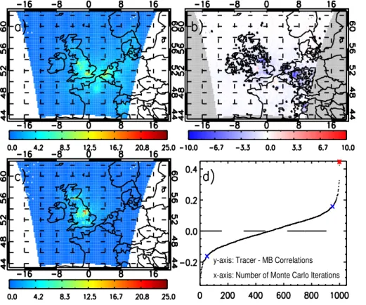
Figure 7a and b highlights the impact of removing point sources as col-umn NO₂ over northern England reduces from 15–25_×1015molecules cm−2 _to

4–5×1015molecules cm−2. The Run E1–OMI MB now ranges between −10 to −6×1015molecules cm−2, while the Run C–OMI MB (Fig. 6a) is between 6–

10_×1015molecules cm−2_{. Therefore, the switch in sign of the biases, of similar}

mag-20

nitude, indicates that the point source emissions play a significant role in the AQUM column NO2budget.

Run E2 aimed to test whether the point sources were responsible for the positive biases in Fig. 6a by using an idealised tracer of the power station emissions. Figure 7c shows the JJA tracer column with the OMI AKs applied, where peak columns range 25

(19)

ACPD

14, 21749–21784, 2014

column NO2

R. Pope et al.

Title Page

Tables Figures

◭ ◮

Back Close

Full Screen / Esc

Discussion

P

a

per

|

Discus

sion

P

a

per

|

Discussion

P

a

per

|

Discussion

P

a

per

|

7c suggest that the peak tracer columns overlap with the large Run C–OMI positive biases.

To test this more quantitatively, the spatial correlation between these peak concen-trations from Run E2 were compared against a random tracer-MB (Run C) correlation distribution. The largest 100 tracer column pixels in Fig. 7c were compared against 5

the MBs over the same locations in Fig. 6a, yielding a correlation of 0.45. Then, using a Monte-Carlo approach, a random 100 sample of the Fig. 6a land-based MB pixels (we use land bias pixels only as the biases in Fig. 6a are over land) were correlated against the largest 100 tracer sample. This was repeated 1000 times and then sorted from lowest to highest. The 5th and 95th percentiles were calculated at₋0.162 and 10

0.158, respectively. Our theory is that if the point sources are responsible for the peak Run C–OMI biases, then the peak tracer concentrations, which represent the point source emissions, should be in the same location as the peak biases. By looking at the random samples correlation, we see how the tracer-MB peak value concentration com-pares with randomly sampled MB locations. Since 0.45 is above the 95th percentile, 15

this shows the tracer-MB peak correlation value is significant (is actually the greatest correlation – see Fig. 7d) and that AQUM’s representation of point source emissions are linked to the AQUM overestimation of column NO2 in northern England and

Scot-land.

4.4 Sensitivity to heterogeneous removal of N2O5

20

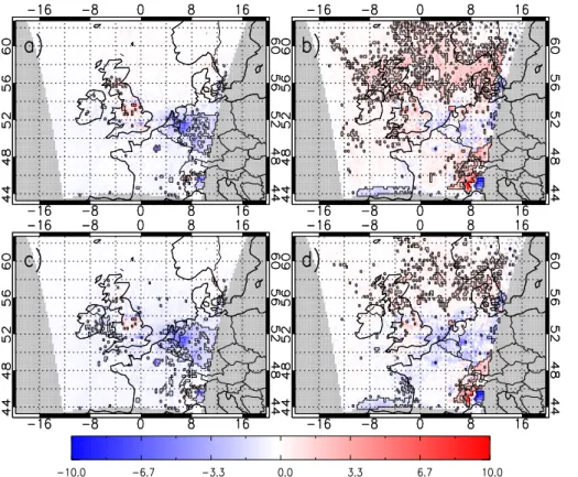
Figure 8 shows the winter and summer MBs between AQUM (with LBCs from GEMS) and OMI when heterogeneous hydrolysis of N2O5 is implemented in the model with

γ =_{0.001 (Run N}₂_O₅_{Low) and}_γ=_{0.02 (Run N}₂_O₅_{High). In the Run C summer case}

(see Fig. 4a) there are positive northern England and Scotland biases of around 5– 10×1015molecules cm−2. We have shown that these positive biases are likely linked to

25

AQUM’s representation of point source emissions. However, by introducing N2O5

(20)

ACPD

14, 21749–21784, 2014

column NO2

R. Pope et al.

Title Page

Tables Figures

◭ ◮

Back Close

Full Screen / Esc

Discussion

P

a

per

|

Discus

sion

P

a

per

|

Discussion

P

a

per

|

Discussion

P

a

per

|

and 50–60◦_{N) decreases from 3.68}

×1015 to 3.39×1015molecules cm−2 and FGE

(over UK domain 8◦_W–2◦_{E and 50–60}◦_{N) also reduces slightly. In Run N}

2O5High

(Fig. 8c) many of the positive biases over point sources are now insignificant and the RMSE decreases to 3.08×1015molecules cm−2. However, over parts of continental

Europe the intensity and spread of negative biases has increased, thus suggesting 5

that γ=_{0.02 might be too strong an uptake here. The FGE does go up slightly to}

0.67 and we suspect that this is due to the introduction of negative biases over rela-tively clean or moderately polluted areas (e.g. the Irish Sea and parts of the continent). Note that the correction of errors of large magnitude (e.g. over point sources) reduces RMSE because this metric penalises the large deviations between the model and 10

the satellite-retrieved columns, while the introduction of errors of low magnitude over less polluted areas might increase the normalised errors given by FGE. The changes at the point source locations are most significant because of the large emissions of NOx and aerosols suitable for this heterogeneous process to take place. Therefore,

we suggest that while AQUM’s representation of point sources results in the sum-15

mer northern England/Scotland positive biases, including N2O5heterogeneous

chem-istry with γ=_{0.02 will partially account for this. In winter, the positive biases seen in}

Fig. 4b, 2–5_×1015molecules cm−2_{, decrease as} _γ _{increases, similarly as found for}

summer. In Run N2O5Low (Fig. 8b) the spatial spread of significantly positive biases

is only partially reduced, resulting in small decreases of RMSE (from 5.12×1015 to

20

5.05_×1015molecules cm−2_{) and FGE (from 0.63 to 0.62). For Run N}

2O5High (Fig. 8d)

the cluster of significantly positive biases has decreased spatially yielding the best comparisons, with RMSE and FGE values of 4.48×1015molecules cm−2and 0.60,

re-spectively.

5 Conclusions 25

We have successfully used OMI satellite observations of column NO2 over the UK to

(21)

ACPD

14, 21749–21784, 2014

column NO2

R. Pope et al.

Title Page

Tables Figures

◭ ◮

Back Close

Full Screen / Esc

Discussion

P

a

per

|

Discus

sion

P

a

per

|

Discussion

P

a

per

|

Discussion

P

a

per

|

which had only used surface data. In order to do this we have looked in detail at the satellite errors (random, systematic and smoothing) and derived an algorithm which reduces the retrieval random error component when averaging retrievals. This allows more critical AQUM-satellite comparisons as the time average random error component can be reduced by 30–90 % in all seasons.

5

Based on the summer and winter comparisons, the standard (operational) AQUM overestimates column NO₂ over northern England/Scotland by 5– 10_×1015molecules cm−2_{and over the northern domain by 2–5}

×1015molecules cm−2.

The use of a diﬀ_{erent set of lateral boundary conditions (from the MACC reanalysis),}

which are known to increase AQUM’s surface ozone positive bias (Savage et al., 2013), 10

also increases the error in the NO₂columns. The AQUM column NO₂is increased, es-pecially in winter, by 2–5×1015molecules cm−2, resulting in poorer comparisons with

OMI.

From multiple sensitivity experiments on the UK NO_xpoint source emissions we con-clude that it was AQUM’s representation of these emissions which caused the northern 15

England/Scotland summer biases. By emitting an idealised tracer in the NOx points

sources we found a significant correlation of the peak tracer columns to the AQUM – OMI MBs. Finally, introducing N₂O₅ heterogeneous chemistry in AQUM improves the AQUM–OMI comparisons in both seasons. In winter, the spatial extent of positive bi-ases, 2–5×1015molecules cm−2, decreases. In summer, the northern England biases

20

decrease both spatially and in magnitude from 5–10 to 0–5_×1015molecules cm−2_.

Therefore, this suggests that in summer the AQUM’s representation of NOx point

sources is inaccurate but can be partially masked by the introduction of N2O5

het-erogeneous chemistry.

As this study has shown the potential use of satellite observations, along with the 25

time-averaged random error algorithm, to evaluate AQUM, the data could be used in future to evaluate operation air quality forecasts. We also show that the heterogeneous loss of N2O5 on aerosol is an important sink of NO2 and should be included in the

(22)

ACPD

14, 21749–21784, 2014

column NO2

R. Pope et al.

Title Page

Tables Figures

◭ ◮

Back Close

Full Screen / Esc

Discussion

P

a

per

|

Discus

sion

P

a

per

|

Discussion

P

a

per

|

Discussion

P

a

per

|

Appendix A

The equations for mean bias (MB), root mean square error (RMSE), modified nor-malised mean bias (MNMB) and the fractional gross error (FGE) are given here, where

f is the model output,ois the satellite measurements,Nis the total number of elements andi is the index. Mean Bias (MB):

5

MB = 1 N

X

i

(fi−oi) (A1)

Modified Normalised Mean Bias (MNMB):

MNMB = 2 N

X(f_i−o_i) fi+oi

(A2)

Root Mean Square Error (RMSE):

RMSE = s

1

N X

i

(f_i−oi)2 (A3)

10

Fractional Gross Error (FGE):

FGE = 2 N

X

i

fi−oi

f_i+o_i

(A4)

Acknowledgements. We acknowledge the use of the Tropospheric Emissions Monitoring In-ternet Service (TEMIS) OMI dataset used in this study. This work was supported by the UK Natural Environment Research Council (NERC) and National Centre for Earth Observation

15

(NCEO). Richard Pope thanks the NCEO for a Ph.D. studentship to undertake this work. We are grateful to Ben Johnson of the Met Oﬃ_{ce who provided advice for the implementation of}

(23)

ACPD

14, 21749–21784, 2014

column NO2

R. Pope et al.

Title Page

Tables Figures

◭ ◮

Back Close

Full Screen / Esc

Discussion

P

a

per

|

Discus

sion

P

a

per

|

Discussion

P

a

per

|

Discussion

P

a

per

|

References

Bellouin, N., Rae, J., Jones, A., Johnson, C., Haywood, J., and Boucher, O.: Aerosol forc-ing in the Climate Model Intercomparison Project (CMIP5) simulations by HadGEM2-ES and the role of ammonium nitrate, J. Geophys. Res.-Atmos., 116, D20206, doi:10.1029/2011JD016074, 2011. 21760

5

Blond, N., Boersma, K. F., Eskes, H. J., van der A, R. J., Van Roozendael, M., De Smedt, I., Bergametti, G., and Vautard, R.: Intercomparison of SCIAMACHY nitrogen dioxide observa-tions, in situ measurements and air quality modeling results over Western Europe, J. Geo-phys. Res.-Atmos., 112, D10311, doi:10.1029/2006JD007277, 2007. 21752

Boersma, K., Eskes, H., and Brinksma, E.: Error analysis for tropospheric NO₂ retrieval from

10

space, J. Geophys. Res.-Atmos., 109, D04311, doi:10.1029/2003JD003962, 2004. 21756, 21757

Boersma, K. F., Eskes, H. J., Veefkind, J. P., Brinksma, E. J., van der A, R. J., Sneep, M., van den Oord, G. H. J., Levelt, P. F., Stammes, P., Gleason, J. F., and Bucsela, E. J.: Near-real time retrieval of tropospheric NO₂from OMI, Atmos. Chem. Phys., 7, 2103–2118,

15

doi:10.5194/acp-7-2103-2007, 2007. 21758

Boersma, K., Jacob, D., Bucsela, E., Perring, A., Dirksen, R., van der A, R., Yantosca, R., Park, R., Wenig, M., Bertram, T., and Cohen, R.: Validation of {OMI} tropospheric {NO2} observations during INTEX-B and application to constrain emissions over the eastern United States and Mexico, Atmos. Environ., 42, 4480–4497, doi:10.1016/j.atmosenv.2008.02.004,

20

2008. 21753, 21754

Boersma, K. F., Jacob, D. J., Trainic, M., Rudich, Y., DeSmedt, I., Dirksen, R., and Eskes, H. J.: Validation of urban NO₂ concentrations and their diurnal and seasonal variations observed from the SCIAMACHY and OMI sensors using in situ surface measurements in Israeli cities, Atmos. Chem. Phys., 9, 3867–3879, doi:10.5194/acp-9-3867-2009, 2009. 21752

25

Boersma, K., Braak, R., and van der A, R.: Dutch OMI NO₂ (DOMINO) data product v2.0, Tropospheric Emissions Monitoring Internet Service on-line Documentation, available at: http://www.temis.nl/docs/OMI_NO2_HE5_2.0_2011.pdf (last access: June 2014), KNMI, the Netherlands, 2011a. 21753, 21755

Boersma, K. F., Eskes, H. J., Dirksen, R. J., van der A, R. J., Veefkind, J. P., Stammes, P.,

Huij-30

(24)

ACPD

14, 21749–21784, 2014

column NO2

R. Pope et al.

Title Page

Tables Figures

◭ ◮

Back Close

Full Screen / Esc

Discussion

P

a

per

|

Discus

sion

P

a

per

|

Discussion

P

a

per

|

Discussion

P

a

per

|

An improved tropospheric NO₂ column retrieval algorithm for the Ozone Monitoring Instru-ment, Atmos. Meas. Tech., 4, 1905–1928, doi:10.5194/amt-4-1905-2011, 2011b. 21753 Braak, R.: Row Anomaly Flagging Rules Lookup Table, KNMI Technical Document

TN-OMIE-KNMI-950, KNMI, the Netherlands, 2010. 21754

Curier, R., Kranenburg, R., Segers, A., Timmermans, R., and Schaap, M.: Synergistic use of {OMI} {NO₂} tropospheric columns and LOTOS?EUROS to evaluate the {NO_x} emission

5

trends across Europe, Remote Sens. Environ., 149, 58–69, doi:10.1016/j.rse.2014.03.032, 2014. 21752

DEFRA: Automatic Urban and Rural Network (AURN), available at: http://uk-air.defra.gov.uk/ networks/network-info?view=_{aurn (last access: 2014), DEFRA, UK, 2012.}

Eskes, H. J. and Boersma, K. F.: Averaging kernels for DOAS total-column satellite retrievals,

10

Atmos. Chem. Phys., 3, 1285–1291, doi:10.5194/acp-3-1285-2003, 2003. 21754

Fitzgerald, J. W.: Approximation formulas for the equilibrium size of an aerosol particle as a function of its dry size and composition and the ambient relative humidity, J. Appl. Me-teorol., 14, 1044–1049, 1975. 21763

Foley, K. M., Roselle, S. J., Appel, K. W., Bhave, P. V., Pleim, J. E., Otte, T. L., Mathur, R.,

Sar-15

war, G., Young, J. O., Gilliam, R. C., Nolte, C. G., Kelly, J. T., Gilliland, A. B., and Bash, J. O.: Incremental testing of the Community Multiscale Air Quality (CMAQ) modeling system ver-sion 4.7, Geosci. Model Dev., 3, 205–226, doi:10.5194/gmd-3-205-2010, 2010. 21752 Han, K., Lee, C., Lee, J., Kim, J., and Song, C.: A comparison study between model-predicted

and OMI-retrieved tropospheric NO₂ columns over the Korean peninsula, Atmos. Environ.,

20

45, 2962–2971, 2011. 21752, 21763

HoC: House of Commons Environmental Audit Report (HCEA): Air Quality: Vol 1 (2009–2010), availabale at: http://www.publications.parliament.uk/pa/cm200910/cmselect/cmenvaud/229/ 229i.pdf (last access: February 2014), House of Commons, London, UK, 2010. 21751 Hollaway, M. J., Arnold, S. R., Challinor, A. J., and Emberson, L. D.: Intercontinental

trans-25

boundary contributions to ozone-induced crop yield losses in the Northern Hemisphere, Bio-geosciences, 9, 271–292, doi:10.5194/bg-9-271-2012, 2012. 21751

Hollingsworth, A., Engelen, R., Benedetti, A., Dethof, A., Flemming, J., Kaiser, J., Morcrette, J., Simmons, A., Textor, C., Boucher, O., Chevallier, F., Rayner, P., Elbern, H., Eskes, H., Granier, C., Peuch, V.-H., Rouil, L., and Schultz, M. G.: Toward a monitoring and forecasting system

30

(25)

ACPD

14, 21749–21784, 2014

column NO2

R. Pope et al.

Title Page

Tables Figures

◭ ◮

Back Close

Full Screen / Esc

Discussion

P

a

per

|

Discus

sion

P

a

per

|

Discussion

P

a

per

|

Discussion

P

a

per

|

Huijnen, V., Eskes, H. J., Poupkou, A., Elbern, H., Boersma, K. F., Foret, G., Sofiev, M., Valdebenito, A., Flemming, J., Stein, O., Gross, A., Robertson, L., D’Isidoro, M., Kiout-sioukis, I., Friese, E., Amstrup, B., Bergstrom, R., Strunk, A., Vira, J., Zyryanov, D., Mau-rizi, A., Melas, D., Peuch, V.-H., and Zerefos, C.: Comparison of OMI NO₂ tropospheric columns with an ensemble of global and European regional air quality models, Atmos. Chem. Phys., 10, 3273–3296, doi:10.5194/acp-10-3273-2010, 2010. 21751, 21755

5

Inness, A., Baier, F., Benedetti, A., Bouarar, I., Chabrillat, S., Clark, H., Clerbaux, C., Coheur, P., Engelen, R. J., Errera, Q., Flemming, J., George, M., Granier, C., Hadji-Lazaro, J., Huijnen, V., Hurtmans, D., Jones, L., Kaiser, J. W., Kapsomenakis, J., Lefever, K., Leitão, J., Razinger, M., Richter, A., Schultz, M. G., Simmons, A. J., Suttie, M., Stein, O., Thépaut, J.-N., Thouret, V., Vrekoussis, M., Zerefos, C., and the MACC team: The MACC reanalysis: an 8 yr data

10

set of atmospheric composition, Atmos. Chem. Phys., 13, 4073–4109, doi:10.5194/acp-13-4073-2013, 2013. 21761

Irie, H., Kanaya, Y., Akimoto, H., Tanimoto, H., Wang, Z., Gleason, J. F., and Bucsela, E. J.: Validation of OMI tropospheric NO₂ column data using MAX-DOAS measurements deep inside the North China Plain in June 2006: Mount Tai Experiment 2006, Atmos. Chem. Phys.,

15

8, 6577–6586, doi:10.5194/acp-8-6577-2008, 2008. 21754

Lauer, A., Dameris, M., Richter, A., and Burrows, J. P.: Tropospheric NO₂columns: a compari-son between model and retrieved data from GOME measurements, Atmos. Chem. Phys., 2, 67–78, doi:10.5194/acp-2-67-2002, 2002. 21751

Macintyre, H. L. and Evans, M. J.: Sensitivity of a global model to the uptake of N₂O₅ by

20

tropospheric aerosol, Atmos. Chem. Phys., 10, 7409–7414, doi:10.5194/acp-10-7409-2010, 2010. 21762

Magi, B. I. and Hobbs, P. V.: Eﬀ_{ects of humidity on aerosols in southern Africa during the}

biomass burning season, J. Geophys. Res.-Atmos., 108, 8495, doi:10.1029/2002JD002144, 2003. 21763

25

Monks, S., Arnold, S., and Chipperfield, M.: Evidence for El Niño–Southern Oscillation (ENSO) influence on Arctic CO interannual variability through biomass burning emissions, Geophys. Res. Lett., 39, L14804, doi:10.1029/2012GL052512, 2012. 21751

O’Connor, F. M., Johnson, C. E., Morgenstern, O., Abraham, N. L., Braesicke, P., Dalvi, M., Folberth, G. A., Sanderson, M. G., Telford, P. J., Voulgarakis, A., Young, P. J., Zeng, G.,

30

(26)

ACPD

14, 21749–21784, 2014

column NO2

R. Pope et al.

Title Page

Tables Figures

◭ ◮

Back Close

Full Screen / Esc

Discussion

P

a

per

|

Discus

sion

P

a

per

|

Discussion

P

a

per

|

Discussion

P

a

per

|

Part 2: The Troposphere, Geosci. Model Dev., 7, 41–91, doi:10.5194/gmd-7-41-2014, 2014. 21760

Pope, R., Savage, N., Chipperfield, M., Arnold, S., and Osborn, T.: The influence of synoptic weather regimes on UK air quality: analysis of satellite column NO₂, Atmos. Sci. Lett., 15, 211–217, doi:10.1002/asl2.492, 2014. 21764

5

Savage, N. H., Pyle, J. A., Braesicke, P., Wittrock, F., Richter, A., Nüß, H., Burrows, J. P., Schultz, M. G., Pulles, T., and van Het Bolscher, M.: The sensitivity of Western European NO₂ columns to interannual variability of meteorology and emissions: a model – GOME study, Atmos. Sci. Lett., 9, 182–188, 2008. 21751

Savage, N. H., Agnew, P., Davis, L. S., Ordóñez, C., Thorpe, R., Johnson, C. E., O’Connor, F. M.,

10

and Dalvi, M.: Air quality modelling using the Met Oﬃ_{ce Unified Model (AQUM OS24-26):}

model description and initial evaluation, Geosci. Model Dev., 6, 353–372, doi:10.5194/gmd-6-353-2013, 2013. 21751, 21752, 21753, 21759, 21760, 21761, 21762, 21763, 21765, 21766, 21769

Seigneur, C., Pun, B., Pai, P., Louis, J.-F., Solomon, P., Emery, C., Morris, R., Zahniser, M.,

15

Worsnop, D., Koutrakis, P., White, W., and Tombach, I.: Guidance for the performance eval-uation of three-dimensional air quality modeling systems for particulate matter and visibility, J. Air Waste Manage., 50, 588–599, 2000. 21752

Steinbacher, M., Zellweger, C., Schwarzenbach, B., Bugmann, S., Buchmann, B., Ordonez, C., Prevot, A., and Hueglin, C.: Nitrogen oxide measurements at rural sites in Switzerland:

20

bias of conventional measurement techniques, J. Geophys. Res.-Atmos., 112, D11307, doi:10.1029/2006JD007971, 2007. 21765

Tie, X., Emmons, L., Horowitz, L., Brasseur, G., Ridley, B., Atlas, E., Stround, C., Hess, P., Klonecki, A., Madronich, S., Talbot, R., and Dibb, J.: Eﬀ_{ect of sulfate aerosol on tropospheric}

NO_xand ozone budgets: model simulations and TOPSE evidence, J. Geophys. Res.-Atmos.,

25

108, 2156–2202, doi:10.1029/2001JD0015082003. 21762

van Noije, T. P. C., Eskes, H. J., Dentener, F. J., Stevenson, D. S., Ellingsen, K., Schultz, M. G., Wild, O., Amann, M., Atherton, C. S., Bergmann, D. J., Bey, I., Boersma, K. F., Butler, T., Cofala, J., Drevet, J., Fiore, A. M., Gauss, M., Hauglustaine, D. A., Horowitz, L. W., Isak-sen, I. S. A., Krol, M. C., Lamarque, J.-F., Lawrence, M. G., Martin, R. V., Montanaro, V.,

30

(27)

simula-ACPD

14, 21749–21784, 2014

column NO2

R. Pope et al.

Title Page

Tables Figures

◭ ◮

Back Close

Full Screen / Esc

Discussion

P

a

per

|

Discus

sion

P

a

per

|

Discussion

P

a

per

|

Discussion

P

a

per

|

tions of tropospheric NO₂compared with GOME retrievals for the year 2000, Atmos. Chem. Phys., 6, 2943–2979, doi:10.5194/acp-6-2943-2006, 2006. 21751

Varutbangkul, V., Brechtel, F. J., Bahreini, R., Ng, N. L., Keywood, M. D., Kroll, J. H., Fla-gan, R. C., Seinfeld, J. H., Lee, A., and Goldstein, A. H.: Hygroscopicity of secondary or-ganic aerosols formed by oxidation of cycloalkenes, monoterpenes, sesquiterpenes, and re-lated compounds, Atmos. Chem. Phys., 6, 2367–2388, doi:10.5194/acp-6-2367-2006, 2006.

5

21763

Velders, G. J., Granier, C., Portmann, R. W., Pfeilsticker, K., Wenig, M., Wagner, T., Platt, U., Richter, A., and Burrows, J. P.: Global tropospheric NO₂ column distributions: comparing three-dimensional model calculations with GOME measurements, J. Geophys. Res.-Atmos.,

675

106, 12643–12660, 2001. 21751