THE CO-INFLUENCE OF THE SEA BREEZE AND THE COASTAL UPWELLING AT
CABO FRIO: A NUMERICAL INVESTIGATION USING COUPLED MODELS
Flávia Noronha Dutra Ribeiro1, Jacyra Soares2 and Amauri Pereira de Oliveira3
1Universidade de São Paulo Instituto de Astronomia, Geofísica e Ciências Atmosféricas
Departamento de Ciências Atmosféricas - (IAG-CA/USP) (Rua do Matão, 1226, 05508-090 São Paulo, SP, Brasil)
E-mail: fndutra@model.iag.usp.br
2
Universidade de São Paulo Instituto de Astronomia, Geofísica e Ciências Atmosféricas Laboratório de Interação Ar-mar Grupo de Micrometeorologia
Departamento de Ciências Atmosféricas (IAG-CA/USP) (Rua do Matão, 1226, 05508-090 São Paulo, SP, Brasil)
E-mail: jacyra@usp.br
3
Universidade de São Paulo Instituto de Astronomia, Geofísica e Ciências Atmosféricas Grupo de Micrometeorologia
Departamento de Ciências Atmosféricas (IAG-CA/USP) (Rua do Matão, 1226, 05508-090 São Paulo, SP, Brasil)
E-mail: apdolive@usp.br
A
B S T R A C TA coupled atmospheric-oceanic model was used to investigate whether there is a positive feedback between the coastal upwelling and the sea breeze at Cabo Frio – RJ (Brazil). Two experiments were performed to ascertain the influence of the sea breeze on the coastal upwelling: the first one used the coupled model forced with synoptic NE winds of 8 m s-1 and the sign of the sea breeze circulation was set by the atmospheric model; the second experiment used only the oceanic model with constant 8 m s-1 NE winds. Then, to study the influence of the coastal upwelling on the sea breeze, two more experiments were performed: one using a coastal upwelling representative SST initial field and the other one using a constant and homogeneous SST field of 26°C. Finally, two more experiments were conducted to verify the influence of the topography and the spatial distribution of the sea surface temperature on the previous results. The results showed that the sea breeze can intensify the coastal upwelling, but the coastal upwelling does not intensify the sea breeze circulation, suggesting that there is no positive feedbackbetween these two phenomena at Cabo Frio.
R
E S U M OUm modelo acoplado atmosférico-oceânico foi usado para investigar se há retroalimentação positiva entre a ressurgência costeira e a brisa marítima em Cabo Frio – RJ (Brasil). Dois experimentos foram realizados para verificar a influência da brisa marítima na ressurgência costeira: o primeiro usou o modelo acoplado, forçado com vento de escala sinótica de NE e 8 m s-1, e o sinal da brisa foi dado pelo modelo atmosférico; o segundo utilizou apenas o modelo oceânico com vento constante de NE e 8 m s-1. A fim de estudar a influência da ressurgência costeira na brisa marítima, mais dois experimentos foram realizados com o modelo acoplado: um com um campo inicial de temperatura da superfície do mar (TSM), representativo da ocorrência de ressurgência costeira; e o outro com um campo constante e homogêneo de TSM de 26°C. Por fim, mais dois experimentos foram feitos para verificar a influência da topografia e da distribuição espacial da temperatura da superfície do mar nos resultados anteriores. Os resultados mostraram que a brisa pode intensificar a ressurgência, mas a ressurgência não intensifica a brisa, sugerindo não haver em Cabo Frio, retroalimentação positiva entre esses dois fenômenos.
Descriptors: Coupled numerical model, Coastal upwelling, Sea breeze, Local atmospheric circulation.
I
NTRODUCTIONCabo Frio is located on the southeastern Brazilian coast, at approximately 23°S and 42°W. Even though it is located onthe western border of the Atlantic Ocean, this area often presents the low sea surface temperatures (SST) characteristic of coastal upwelling. This phenomenon is frequently observed at Cabo Frio due to a semi-permanent large scale high pressure center (the South Atlantic High) that gives rise to the prevailing NE winds. This wind field lies mainly parallel to the coast, with the coast to its right. In the southern hemisphere, this wind field causes the seaward transport of the coastal water (Ekman transport) which allows deeper waters to surface, decreasing the SST near the coast to 13-14°C (FRANCHITO et al., 1998).
Coastal upwelling is usually stronger near Cabo Frio than in other areas of the Brazilian southeastern coast because of its particular coastline geometry and bottom topography (RODRIGUES; LORENZZETTI, 2001) and the availability of Southeast Atlantic Central Water at the shelf-break, especially during summer (CAMPOS et al., 1995). Thisis highly important because it brings nutrient rich water to the coast (CARBONEL; VALENTIN, 1998) and enhances fishery production (DINIZ et al., 2003). The colder SST also has an impact on atmospheric processes and weather conditions.
Due to the passage of cold fronts, every 5 to 10 days on average, the wind direction changes from NE to SW. This change disrupts the mechanism that sustains the coastal upwelling; increasing SST values once again (DOURADO; OLIVEIRA, 2001).
Since it is a coastal area, the atmospheric circulation pattern at Cabo Frio is greatlyinfluenced by the sea breeze, which is also an important phenomenon, since it affects local weather and air quality (MILLER et al., 2003). The sea breeze is a mesoscale circulation system caused by a temperature gradient between the air over the continent andthat over the ocean. During the day, the soil is heated by the solar radiation and the air temperature near the continental surface rises rapidly. The SST changes much more slowly and thus the air over the ocean remains cooler than that over the continent, producing a horizontal thermal gradient. The sea breeze is characterized by shoreward flow near the surface, rising air currents over the continent, usually a seaward return flow at higher altitudes and diffuse sinking currents over the ocean, composing a vertically rotating cell (MILLER et al., 2003).
Miller et al. (2003) reviewed the research on the forcing mechanisms, structure and related phenomena, life cycle, forecasting, and impacton air quality of the sea breeze system and suggested that the following factors should be included in a complete
physical model of the system: diurnal variation of the ground temperature, diffusion of heat, static stability, Coriolis force, diffusion of momentum, topography (including the size and shape of the landmass and the details of the coastline) and prevailing wind. The author also suggested that the coastal upwelling intensifies the sea breeze circulation, since it decreases the values of the SST near the coast and, consequently, increases the horizontal thermal gradient that generates that circulation.
Mizzi and Pielke (1984) used a numerical atmospheric model to study the effect of an ocean surface temperature gradient on the mesoscale atmospheric circulation and, among other observations, notedthat the coastal upwelling does not intensify the sea breeze circulation. The authors suggested that the causes of this were the increased stability and the decreased atmospheric horizontal thermal gradient near the surface, caused by advection of cooler marine air. They also affirmed that the spatial scale of the ocean thermal gradient was not large enough to have a significant effect upon the mesoscale pressure gradient, since the coastal upwelling presents low SST values in a relatively narrow area of the ocean near the coast.
In order to study the effect of coastal upwelling on the sea breeze circulation at Cabo Frio, Franchito et al. (1998) used a three-dimensional non-linear primitive equation atmospheric model with the SST held constant and homogeneous. Four experiments were performed, simulating the summer, fall, winter and spring periods, and the wind fields generated were then used to force a 2-layer finite element oceanic model. The atmospheric model results showed that when the upwelling is stronger and produces a higher temperature gradient between the ocean and the continent (summer and spring), the sea breeze is also stronger. The oceanic model results showed that, when the wind field generated by the atmospheric model is added to a constant NE wind of 6 m s-1, the upwelling is enhanced. Therefore, the results suggest that there is positivefeedback between the upwelling and the sea breeze at Cabo Frio.
Oda (1997) determined hourly averages of a series of 10 years of hourly data of wind at 10 m height and SST, taken near the cape (22.90°S and 42.02°W approximately). The author noted that the SST is possibly modulated by the diurnal atmospheric circulation cycle. It was seen, further, that the sea breeze increases the zonal component of the wind and decreases its meridional component and that the land breeze occurs only during April, May and June (fall).
Cabo Frio, since the months with greater values of the zonal component of the wind are also the months with the lowerSST values.
The objective of this study is to investigate the influence of the sea breeze on the coastal upwelling and the influence of the coastal upwelling on the sea breeze, at Cabo Frio, by using a coupled atmospheric-ocean model.
Numerical Models
The atmospheric TVM-NH model has been successfully used by many authors to study sea breezes (MARTÍN et al., 2000; CLAPPIER et al., 2000; ORGAZ; FORTES, 1998) and even lake-breezes (STIVARI et al., 2003) in many areas. It is a finite difference numerical model based on the vorticity equations,is non-hydrostatic and uses sigma coordinates (THUNIS, 1995). The oceanic model is based on the model used by Carbonel (2003) and it is able to reproduce the most important features of the coastal upwelling phenomenon at Cabo Frio with a good degree of approximation.
Oceanic numerical model
The model is based on that described by Carbonel (2003). It has a lower layer with constant temperature and no pressure gradients and an upper layer where the governing equations are the vertically-integrated non-linear equations of momentum, continuity and transport of SST, as follows:
where h is the upper layer thickness, u and v are the velocity components in the zonal and meridional directions, respectively, U and V are the transport components (U=h.u;V=h.v), fis the Coriolis parameter,
g is the acceleration due to gravity, SST is the
temperature at the sea-surface, r is the Rayleigh friction coefficient,
θ
is the thermal expansion coefficient and the density coefficients are defined as1
σ= −µ,
( µ )
µ µ σ =
−
and u l ρ µ
ρ
= , where ρuis the upper
layer density, ρlis the inert layer density.
The entrainment velocity (
w
e) is defined as( )2
i e e e H h w t H −
= when h≤He and we=owhen h > He. He
is the entrainment thickness, te is the entrainment time scale and Hi is the initial upper layer thickness.
The source or sink of heat across the interface (s) is defined as
U SST l V SST l
i i
T T
s H H
x h y h
∂ − ∂ −
= +
∂ ∂
, where l
Tis the
initial temperature of the inert layer. The surface heat flux (Q) is defined as 2
SST u i s H T Q t h − =
when the
model is uncoupled, where Tuis the initial temperature
of the upper layer and
s
t is the surface heat flux time
scale.
When the model is uncoupled, the wind stress (τi) is defined as air
i C w WD i
τ ρ= , i=x,y, where
air
ρ is the air density,
D
C is the drag coefficient, wi is
the wind component in direction i, as wi = ua when i =
x and wi = va when i = y. |W| is the wind velocity. The boundaries are of two types: land and ocean. At the land type boundary, the velocity and transport components normal to the boundary are set to zero and h and SST are homogeneous. At the ocean type boundary, the weakly-reflective boundary condition described by Verboom and Slob (1984) and also discussed by Van Dongeren and Svendsen (1997) is used.
The numerical approximation of this model uses the finite difference method, with a forward difference in time with a dissipative interface and a centered difference in space. The velocity and transport values, u and U respectively, are placed between the grid points (i, j) and (i, j+1) in the grid cell; v and V are placed between (i, j) and (i+1, j) and the SST and the thickness (h) are placed at the center of the grid cell.
The order of calculation is: first the heat exchanges s and Q are calculated; then the SST and the pressure gradient; after that, the transport components (U and V) and finally, the thickness of the upper layer (h). The current components are then calculated as the divisionof the transport components by the thickness h. The constant parameters and the initial values of the variables are the same as those used by Carbonel (2003) and are listed at Table 1.
U uU vU SST
V U 0
2
x u
h h
f gh r
t x y x x
τ θ σ ρ µ ∂ +∂ +∂ − + ∂ + ∂ + − = ∂ ∂ ∂ ∂ ∂ (1)
V uV vV SST
U V 0
2
y u
h h
f gh r
t x y y y
τ θ σ ρ µ ∂ +∂ +∂ + + ∂ + ∂ + − = ∂ ∂ ∂ ∂ ∂ (2) U V 0 e h w
t x y
∂ +∂ +∂ − =
∂ ∂ ∂ (3)
( )
SST SST SST 1
u v s Q 0
t x y h
∂ + ∂ + ∂ + + =
Table 1. Description of the constant parameters used by the oceanic model.
Parameter Notation Value
Initial upper layer thickness
Hi 30 m
Entrainment thickness
e
H 20 m
Upper layer density ρu 1023 kg m−3
Lower layer density
ρ
l 1026.7 3kg m−
Coriolis parameter
f
5 15.68 10 s− −
− ×
Wind drag coefficient
D
C 3
2.0 10× −
Air density ρair
1.2kg m−3
Rayleigh friction coefficient
r 6 1
1.8 10 s× − − Initial upper layer
temperature
u
T 26°C
Lower layer temperature l
T
14°CThermal expansion
coefficient
θ
4 1
3.0 10 C× −° −
Entrainment time scale
e
t
½ daySurface heat flux time
scale
t
s12 days
Time step ∆t 600 s
Atmospheric numerical model
The non-hydrostatic version of the TVM model, developed by Thunis (1995), is three-dimensional, follows the Boussinesq approximations of the vorticity equations, obtained from the basic Reynolds-averaged equations of motion, and uses sigma coordinates. The vorticity approach makes the pressure and the density variables drop out of the prognostic equations.
The vertical grid is structured as follows: soil parameters at the bottom boundary; the first layer is the surface boundary layer, where the meteorological parameters are calculated by similarity theory equations and, at the other layers, the finite approximation of the hydrodynamic and thermodynamic equations are solved.
The soil parameters are determined in the following order: first the model evaluates solar and infrared radiative fluxes and calculates the net radiation RN; then it obtains the soil heat flux G by the equation
N
G=R −SH−LH- (5)
where SH is the sensible heat flux and LH is the latent heat flux from the previous time step; finally, the surface temperature is computed for all soil types except water by the force-restore method of Deardorff (1978), and specific humidity is computed using the Penmann-Monteith method. For water, when the model is uncoupled, the surface temperature is constant and homogeneous, but when the model is coupled,the time and spatial evolution of the surface temperature is provided by the oceanic model.
The surface boundary layer fluxes are then evaluated by 2 * * * * * air air p air v u
SH C u
LH L u q
τ ρ ρ θ ρ = − = − = − (6)
where τ is the wind stress, Cp is the specific heat at constant pressure, Lv is latent heat of water vaporization, u* is friction velocity, θ* is the potential temperature scaling parameter and q* is the specific humidity scaling parameter.
The values of the fluxes are then used to force the hydrodynamic and thermodynamic equations at the other layers of the domain: the turbulent kinetic energy equation is solved; the diffusion coefficient profiles are obtained; potential temperature, specific humidity and horizontal vorticity equations are solved; the streamfunctions and velocity components are updated; time is advanced and the cycle is repeated. For a more detailed description of the model, see Thunis (1995).
Initial and Boundary Conditions of the Atmospheric Model
Fig. 1. Topography and coastline of the area investigated. The atmospheric model has 6 boundaries: four lateral boundaries, one boundary at the surface and another at the top of the domain. The zero gradient boundary condition is used at the lateral boundaries. At the top, the vorticity, the turbulent kinetic energy and the vertical gradient of the vertical wind component are set to zero and the wind is geostrophic. Also, the 5 upper levels have a filter to avoid reflection at the top of the domain. At the surface, the wind velocity is zero and the surface fluxes are determined as described at the previous section.
The soil type considered here is culture and is homogeneous for the continentalpart of the domain, since a more realistic soil type distribution has little impact on the results (not shown here). The soil parameters for culture are: albedo (15%); emissivity (92%); superficial resistance (300 s m-1); thermal capacity (2.5x10⁷ J m-3 k-1); roughness length (0.2 m); surface initial temperature (299 K); soil temperature at a depth of 10 cm (297 K). For water, the albedo is 9%, the emissivity is 98%, the superficial resistance is 10 s m-1; the thermal capacity is 1.04x10⁹ J m-3 k-1; the roughness length is 0.001 m and the temperatures are constant (for the uncoupled model) or given by the oceanic model (for the coupled model).
The initial conditions involve vertical profiles of potential temperature and wind that are horizontally-homogeneous initialized. The potential temperature vertical profile is shownin Figure 2a and is based on the radiosonde soundings taken at Cabo Frio by Oda (1997) on 01/09/1995, but the wind vertical profile depends on the experiment. The specific humidity is 16.8 g kg-1 near the surface, also based on the soundings taken by Oda (1997), and is set to have an initial logarithmic vertical profile (Fig. 2b). The day of the year is 37 (February 6), representative of summer. All the simulations of the atmospheric model started at 00 local standard time (LST = GMT + 3 hours) and lasted for 30 hours.
Fig. 2. Initial (a) potential temperature and (b) specific humidity vertical profiles for the atmospheric model. Based on Oda (1997).
Coupling Between the Oceanic and Atmospheric Models The oceanic model was developed in the form of a subroutine and set to use the same horizontal grid spacing as the TVM-NH model. When the atmospheric model starts, it calls the oceanic model subroutine that returns a 2-day integration SST field, forced by a constant and horizontally-homogeneous wind field of 8 m s-1 from the NE (Fig. 3). The 2-day period was chosen because it gives enough time for the upwelling phenomenon to become well established in the region. Ikeda et al. (1974) showed that the time lapse between the onset of the NE winds, with magnitude greater than 5 m s-1, and the first appearance of colder upwelling water is about 24 hours. Then the SST field is used by the TVM-NH model to determine the surface heat flux over the ocean. The time step of the TVM-NH and the oceanic models are, respectively, 30 and 600 seconds. Therefore, the SST field remains the same for 20 time steps of the TVM-NH model, and then the oceanic model is called again. The TVM-NH model forces the oceanic model with the wind stress (τ)obtained by Eq. (6) and the surface heat flux (Q) calculated by Eq. 7. The oceanic model then updates the SST field and returns to the TVM-NH model.
Q = G / (ρair C
p) (7)
Numerical Experiments
Two sets of tests were performed. The first set investigates the influence of the sea breeze on the coastal upwelling and is composed of two experiments: one using just the oceanic model, hereafter called the OCEAN experiment, and the other one using the coupled model, hereafter called the COUPLED experiment.
The OCEAN experiment uses a constant and homogeneous NE wind field of 8 m s-1 and was run for 30 hours. The COUPLED experiment uses an initial NE wind field of 8 m s-1, but the temporal and spatial evolution of the wind field is given by the atmospheric model. Both experiments utilized the initial SST field presented inFigure 3.
The second set of tests was performed to study the influence of the coastal upwelling on the sea breeze. The initial wind field was set to zero in order to isolate the sea breeze circulation from the effects of the prevailing wind. The set is formed by 4 experiments, summarized in Table 2.
Table 2. Summary of the initial conditions of the experiments. The initial wind field was set to zero.
Experiment Model Initial SST
field
Topography
EXP1 coupled Figure 3 realistic
EXP2 atmospheric 26°C realistic
EXP3 atmospheric 18°C realistic
EXP4 coupled Figure 3 flat
EXP1 simulates an upwelling case and considers a realistic topography. The case without the
presence of the upwelling phenomenon is simulated by EXP2 that uses a homogeneous SST field of 26°C. EXP3 was performed to analyze the influence of a temperature gradient on the SST field and uses a homogeneous SST field of 18°C. The influence of the topography is investigated by comparing the results of EXP1 and EXP4, since EXP4 considers a flat topography.
R
ESULTSThe Main Results are Presented Below. Influence of the Sea breeze on the Coastal Upwelling
The difference between the SST fields generated by the OCEAN and the COUPLED experiments is presentedinFigure 4a. It is noticeable that, westward from the cape, the SST is cooler in the experiment with the sea breeze circulation (COUPLED) than in the constant wind experiment (OCEAN) but, eastward from the cape, the SST of the COUPLED experiment is higher than the SST of the OCEAN experiment. These differences are caused by the change in the direction of the prevailing wind, due to the sea breeze circulation for the COUPLED experiment (Fig. 4b). The sea breeze increases the component of the wind stress that is parallel to the coast on the western part of the cape and decreases this component on the eastern part.
A similar pattern can be seen in the current fields (Fig. 5). The currents are more intense for the COUPLED experiment (Fig. 5a)in the western part of the domain and less intensein the eastern part than for the OCEAN experiment (Fig. 5b).
Fig. 5. Current field after 30 hours of integration of (a) COUPLED and (b) OCEAN experiments. Influence of the Coastal Upwelling on the Sea Breeze
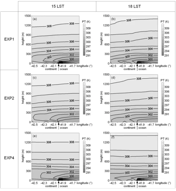
Figure 6 shows the wind field and the air potential temperature field at 15 m height at 15 LST (left column) and 18 LST (right column) for EXP1 to EXP4 (Table 2). Comparing EXP1 and EXP2 (Fig. 6a-d), it is noticeable that, over the continent, the air potential temperature fields of both experiments are similar, but they are different over the ocean, since the initial SST fields are different in thetwo experiments. For EXP2, the air temperature over the ocean remained close to the initial SST temperature, approximately 26°C. The difference between the air temperature at 15 LST and 18 LST shows the inland penetration of the sea breeze. The thicker line represents the 29°C contour line and has penetrated further inland at 18 LST than at 15 LST for both experiments.
The wind field also shows the presence of the sea breeze circulation, since the direction of the wind vectors, near the coastline, is alwayslandward. Some circulation patterns related to the topography can be found, especiallyinthe upper left part of the domain (approximately 22.4°S and 42.4°W). The greater difference between EXP1 and EXP2 is over the ocean, since EXP2 presents SE winds (landward) at almost every point of the domain over the ocean and EXP1 presents great variation in the wind direction, especially in the right part of the domain. This difference is related to the horizontal thermal gradient over the ocean in EXP1 that generates a thermal westward gradient force.
EXP3 (Fig. 6e,f) has a wind field, over the continent, similar to that of EXP1 and, over the ocean, similar to the wind field of EXP2, since EXP3 also used a homogeneous initial SST field. Lower values of temperature penetrated further inlandin EXP3 than in
EXP1. The wind field is also stronger in EXP3 than EXP1, especially as regards the sea breeze circulation.
The air potential temperature field in EXP4 (Fig. 6g,h) is different from that in EXP1 over the continent, since EXP4 considers a flat topography. The wind fieldin EXP4 is weaker than in EXP1 over the continent, where the sea breeze does not circulate. Over the ocean, the wind fields are similar. The air potential temperature field in EXP4 shows that the sea breeze penetrates inland from the coastline less than it does along most of the coastline in EXP1.
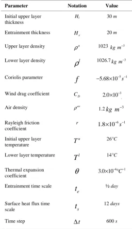
Figure 7 presents the vertical cross-section of the zonal component of the wind over line 1 of Figure 1. The zonal component is the main component of the sea breeze circulation over this line. All the heights given are above ground level.
The circulation near the surface in EXP1 (Fig. 7a,b) has similarities with that in EXP2 (Fig. 7c,d) and is weaker than the circulation in EXP3 (Fig. 7e,f). Above 700 m height, the first 3 experiments present similar fields, but EXP4 does not show the circulation from the east over the continent due to the absence of topographyinthe domain. The sea breeze circulation develops later in EXP4 (Fig. 7g,h), but at 18 LST it is similar to that in EXP1.
Fig. 6. Air temperature (AT) and wind vectors at 15 m height for EXP1 at (a) 15 LST and (b) 18LST, EXP2 at (c) 15 LST and (d) 18 LST, EXP3 at (e) 15 LST and (f) 18 LST and EXP4 at (g) 15 LST and (h) 18 LST. The thicker black line represents the contour line of 29°C and the white line represents the coastline.
Above 700 m, the first 3 experiments present over the continent a circulation from the north related
Fig. 8. Vertical cross-section of the meridional component over line 1 for EXP1 at (a) 15 LST and (b) 18 LST and EXP4 at (c) 15 LST and (d) 18 LST. Contour interval is 0.5 m s-1.
EXP4 also shows a sea breeze circulation that develops later and becomes more intense than in the other experiments, suggesting that the topography of the region induces an earlier but less intense sea breeze.
The meridional component of the wind is the main component of the sea breeze over line 2 (not shown here). As with the results over line 1, the circulation in EXP1 is similar to that in EXP2, with both experiments showing a less intense circulation at 18 LST than at 15 LST. EXP3 once again presents a more intense sea breeze circulation than the other experiments and EXP4 once more presents a later development of the sea breeze, but the circulation becomes more intense at 18 LST than in the other experiments. Between 600 m and 1300 m height, there is a circulation related to the topography that is present in EXP1, EXP2 and EXP3, but not in EXP4.
The vertical cross-sections of the zonal component of the wind over line 2 are presented in Figure 9. There is great similarity between EXP1 (Fig. 9a,b) and EXP2 (not shown here). EXP3 (Fig. 9c,d) shows a more intense circulation between 50 m and 200 m height, but one that is also similar to those of the first two experiments. All the 3 experiments
present a circulation related to the topography, above 900 m height, that is not present in EXP4 (Fig. 9e,f). At 18 LST, EXP4 presents the influence of the coastline on the wind field, since the circulation from the east near the surface suffers the influence of the sea breeze from the eastern part of the domain.
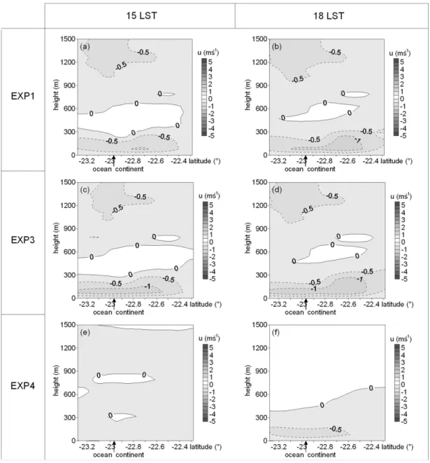
between the latitudes of 42.1°W and 42.0°W) and the contour line of 302 K moved from 42.0°W to 42.54°W, EXP1 thus showing great similarity to EXP2. A similar pattern is to be observed over line 2 (not shown here) but, over line 2, the baroclinicity caused by the topography is more evident.
The air potential temperatures of EXP4 (Fig. 10e,f), above 300 m height, are nearly parallel to the
surface because of the flat topography of the experiment. Near the surface of the continental region the atmosphere is unstable, especially at 15 LST (Fig. 10e). The other experiments show an inclination of the contour lines, mainly over the continent, thus causing the circulation from the east observed at the cross-sections of the zonal component over line 1(Fig. 7).
Fig. 10. Vertical cross-section of the potential temperature over line 1 for EXP1 at (a) 15 LST and (b) 18 LST, EXP2 at (c) 15 LST and (d) 18 LST and EXP4 at (e) 15 LST and (f) 18 LST. Contour interval is 1 K.
Land Breeze
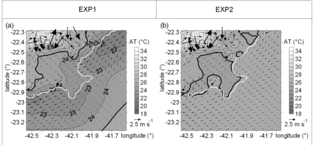
Only EXP1 and EXP2 have been investigated for the following analysis, because EXP1 represents a more realistic coastal upwelling case and EXP2 represents the absence of the coastal upwelling phenomenon. The wind field at 15 m height at 06 LST, after 30 hours of simulation, for EXP1 (Fig. 11a) does not show evidence of the land breeze circulation due to the lack of horizontal thermal gradient inversion (air above the continent cooler than the air above the sea) that generates the land breeze. EXP2 shows a weak horizontal thermal gradient inversion (Fig. 11b)
Fig. 11. Air temperature (AT) and wind vectors at 15 m height after 30 hours of simulation for (a) EXP1 and (b) EXP2. The thicker black line represents the contour lineof 25°C and the white line represents the coastline.
D
ISCUSSIONThe influence of the sea breeze on the coastal upwelling phenomenon was investigated by comparing the results of an oceanic model forced with a constant NE wind field to the results of the coupled oceanic-atmospheric model. The wind field generated by the coupled model, during daytime, showed the development of the sea breeze circulation. This circulation is peculiar to Cabo Frio due to the change in the direction of the coastline from NE-SW to E-W.
Eastward from the cape (NE-SW coastline direction), the influence of the sea breeze on the prevailing NE wind decreases the wind component parallel to the coast, consequently diminishing the intensity of the upwelling. Westward from the cape (E-W coastline direction, around 22.9°S of latitude), the influence of the sea breeze causes an increase in the wind component parallel to the coastline and, consequently, intensifies the upwelling. These results indicate that the sea breeze intensifies the upwelling westward from the cape, but does not intensify it northeastward from the cape (Figs. 4 and 5).
The influence of the upwelling on the sea breeze circulation has been studied comparing the results generated by an experiment with an initial SST field representative of upwelling with those of an experiment using a constant SST field without the presence of the upwelling phenomenon. The vertical cross-sections of the wind components over the two lines across the domain presented similar results for both cases (with and without the presence of upwelling), indicating the absence of any influence of
the upwelling on the sea breeze circulation (Fig. 7a-d). An analysis of the vertical cross-section of the air potential temperature showed that, for both experiments, the horizontal thermal gradient near the surface at the coast decreases with time, as the marine air penetrates inland (Fig. 10). These results are in agreement with those of the work of Mizzi and Pielke (1984).
It was observed that the topography generates an early development of the sea breeze and, in some parts of the domain, increases the inland extension of the breeze (Figs 7g,h and 8c,d).
When the upwelling is represented by a homogeneous SST field of 18°C, the sea breeze circulation is more intense and reaches further inland and offshore than that generated by a more realistic SST spatial distribution, overestimating the sea breeze circulation, because the whole wind field over the continent near the surface is forced towards the continent by the horizontal thermal gradient. The realistic SST field generates a horizontal thermal gradient near the surface that, besides the sea breeze, drives an offshore circulation, towards areas that present larger values of SST.Therefore, the sea breeze circulation generated by a realistic SST field is less intense than when a homogeneous SST field is used (Figs 7e,f and 9c,d).
land breeze circulation, except on some parts of the coastline (Fig. 11).
The sea breeze circulation at Cabo Frio proves to be complex, with three-dimensional features, due to the peculiar coastline and topography.
No evidence for any positive feedback between the coastal upwelling and the sea breeze circulation in this area was found.
A
CKNOWLEDGMENTSWe thank the Brazilian Research Agency CNPq (grants 142007/2005-6 and 305893/2009-2) for funding this work and for the support given by the Fundação de Amparo à Pesquisa do Estado de São Paulo (FAPESP).
R
EFERENCESCAMPOS, E. J. D.; GONÇALVES, J. E.; IKEDA, Y. Water mass characteristics and geostrophic circulation in the South Brazil Bight: Summer of 1991. J. geophys. Res., v. 100, n. 9, p. 18537-18550, 1995.
CARBONEL, C. A. A. H.; VALENTIN, J. L. Numerical modelling of phytoplankton bloom in the upwelling ecosystem of Cabo Frio (Brasil). Ecol. Model., v. 116, p. 135-148, 1998.
CARBONEL, C. A. A. H. Modelling of upwelling-downwelling cycles caused by variable wind in a very sensitive coastal system. Continent. Shelf Res., v. 23, p. 1559-1578, 2003.
CLAPPIER, A.; MARTILLI, A.; GROSSI, P.; THUNIS, P.; PASI, F.; KRUEGER, B. C.; CALPINI, B.; GRAZIANI, G.; VAN DEN BERGH, H. Effect of Sea Breeze on Air Pollution in the Greater Athens Area. Part I: numerical simulations and field observations. J.appl. Met.., v. 39, n. 4, p. 546-562, 2000.
DEARDORFF, J. W. Efficient prediction of ground surface temperature and moisture with inclusion of a layer of vegetation. J. geophys. Res., v. 83, C4, p. 1889-1903, 1978.
DINIZ, A. G.; HAMACHER, C.; WAGENER, A. L. R.; RODRIGUEZ-GONZALEZ, E. Is copperan inhibiting factor for primary production in the upwelling waters of Cabo Frio. J. Braz. Chem. Soc., v. 14, n. 5, p. 815-821, 2003.
DOURADO, M.; OLIVEIRA, A. P. Observational description of the atmospheric and oceanic boundary layer over the Atlantic Ocean. Rev. Bras. Oceanogr., v. 49, n. 1/2, 49-59, 2001.
FRANCHITO, S. H.; RAO, V. B.; STECH, J. L.; LORENZZETTI, J. A. The effect of coastal upwelling on the sea breeze circulation at Cabo Frio, Brazil: a numerical experiment. Ann. Geophysicae, v. 16, p. 866-881, 1998.
FRANCHITO, S. H.; ODA, T. O.; RAO, V. B. E; KAYANO, M. T. Interaction between coastal upwelling and local winds at Cabo Frio, Brazil: an observational study, J. appl. Met. Climatol., v. 47, p. 1590-1598, 2008. IKEDA, Y.; MIRANDA, L. B. de; ROCK, N. J. Observations
on stages of upwelling in the region of Cabo Frio (Brazil) as conducted by continuous surface temperature and salinity measurements. Bolm Inst. Oceanogr., São Paulo, v. 23, p. 33-46, 1974.
MARTÍN, F.; CRESPÍ, S. N.; PALACIOS, M. Simulations of mesoscale circulations in the center of the Iberian Peninsula for thermal low pressure conditions. Part I: Evaluation of the Topography Vorticity-Mode Mesoscale Model. J. appl. Met., v. 40, p. 880-904, 2000. MILLER, S. T. K.; KEIM, B. D.; TALBOT, R. W.; MAO, H.
Sea breeze: structure, forecasting and impacts. Revs. Geophys., v. 41, n. 3, p. 1-31, 2003.
MIZZI, A. P.; PIELKE, R. A. A numerical study of the mesoscale atmospheric circulation during a coastal upwelling event on 23 august 1972. Part I: sensitivity studies. Mon. Weather Rev., v. 112, p. 76 – 90, 1984. ODA, T. O. Influência da ressurgência costeira sobre a
circulação local em Cabo Frio (RJ). 1997. 140 p. Dissertação (Mestrado em Meteorologia), INPE, São Paulo, Brasil, 1997. (in portuguese).
ORGAZ, M. D. M.; FORTES, J. L. Estudo das brisas costeiras na região de Aveiro. In: SIMPÓSIO DE METEOROLOGIA E GEOFÍSICA HISPANO PORTUGUÊS, 1, 1998, Lagos, Portugal. Proceedings ... Lagos, 1998. p. 189-194.
RODRIGUES, R. R.; LORENZZETTI, J. A. A numerical study of the effects of bottom topography and coastline geometry on the Southeast Brazilian coastal upwelling. Continent. Shelf Res., v. 21, p. 371-394, 2001. STIVARI, S. M. S.; OLIVEIRA, A. P.; KARAM, H. A.;
SOARES, J. Patterns of Local Circulation in the Itaipu Lake Area: Numerical Simulations of Lake Breeze. J. appl. Met., v. 42, p. 37-50, 2003.
THUNIS, P. Formulation and evaluation of a nonhydrostatic vorticity mesoscale model. 1995. 151 p. Ph.D Thesis, Institut d’Astronomie et de Géophysique G. Lamaître, Université Catholique de Louvain, Louvain-la-Neuve, Belgium, 1995.
VAN DONGEREN, A. R.; SVENDSEN, I. A. Absorbing-generating boundary condition for shallow water models. J. WatWay, Port, coast. Ocean Engng., Nov./Dec., p. 303-313, 1997.
VERBOOM, G. K.; SLOB, A. Weakly reflective boundary conditions for two-dimensional shallow water flow problems. Delft Laboratory, Publication n. 322, 1984.