Topics on High-Energy Elastic Hadron Scattering
M. J. Menon
Instituto de F´ısica “Gleb Wataghin” Universidade Estadual de Campinas, UNICAMP
13083-970, Campinas, SP, Brazil Received on 15 December, 2004
We review the main results we have obtained in the area of high-energy elastic hadron scattering and presented in this series ofWorkshops on Hadron Interactions. After an introduction to some basic experimental and theoretical concepts, we survey the results reached by means of four approaches: analytic models, model-independent analyses, eikonal models and nonperturbative QCD. Some of the ongoing researches and future perspectives are also outlined.
1
Introduction
“QCD nowadays has a split personality. It em-bodies hard and soft physics, both being hard subjects and the softer the harder.”
Yuri Dokshitzer (2001) [1]
Despite the great success of QCD as the field theory of hadronic interactions, there still remains some open ques-tions and one of them is related to the hadron-hadron scat-tering athigh-energiesandsmall momentum transfer (soft diffraction).
The region of high energies is characterized by scatter-ing of particles with center of mass energy√s >10GeV
∼ 10mp (the proton mass). From the experimental point
of view, diffractive processes are associated with a slow in-crease of the total cross sections, the diffraction pattern in the differential cross section, and rapidity gaps in the plots of pseudo rapidityversusazimuthal angle. In the theoreti-cal context, diffraction means that the initial and final states in the scattering process have the same quantum numbers and, therefore, the exchanged “object” has the vacuum quan-tum numbers (Pomeron). The soft diffractive processes are generally classified as double diffraction dissociation, single diffraction dissociation and elastic scattering. Introductory reviews on the area can be found in Refs. [2-7].
High-energy elastic hadron scattering is the simplest soft diffractive process and, at the same time a topical prob-lem in high-energy physics. Being associated with long distance phenomena perturbative QCD can not be applied. On the other hand, the standard non-perturbative approach starts with the ground state (vacuum), proceeds with bound states (mesons, barions) and eventually reaches the scatter-ing states. However, it is obvious that the vacuum is a non-trivial problem. Moreover, even assuming some vacuum concept, to treat only one gluon field it is necessary to take into account more than 30 invariants, and all that becomes a typical problem of statistical physics, with specific technical approaches, such as Monte Carlo simulation (lattice QCD).
Although bound states may be described, the point is that, presently, we do not know how to calculate elastic scattering amplitudes from a pure nonperturbative QCD formalism.
At this stage, phenomenology certainly plays an impor-tant role in the search for connections between experimental data, model descriptions, and the possible development of new calculational schemes in the underlying theory (QCD). Here, however, we are faced with another kind of problem, namely, the wide variety of model descriptions, based on different ideas and approaches, not always giving enough support for the development of novel calculational schemes well founded on QCD.
Based on the above facts, our main strategy in the in-vestigation of the elastic sector is to search for model inde-pendent informationthat may be extracted from the experi-mental data, through approaches that have well established bases on the General Principles, theorems and bounds from axiomatic quantum field theory (theanalytic approach). Si-multaneously, we attempt to construct phenomenological models, in agreement with the above Principles and con-nected, in some way, with the underlying dynamics of QCD. In this review, it is presented some results we have ob-tained in the area of elastic scattering in the last years, with focus on high-energy proton-proton (pp) and antiproton-proton (pp) elastic scattering. The manuscript is organized¯
as follows. In Sec. 2 we recall some basic experimental and theoretical concepts, defining also our notation. In Secs. 3, 4, 5, and 6 we present the main results we have obtained throughout the analytic approach, model independent analy-ses, eikonal models and nonperturbative QCD, respectively. In Sec. 7 we discuss some perspectives in the area, from both experimental and theoretical points of view. A summary and some final remarks are the contents of Sec. 8.
2
Basic concepts
princi-ples, high-energy theorems, and the main formulas associ-ated with two basic pictures, usually referred as s-channel (geometrical/optical picture) and t-channel (exchange pic-ture) [3-7].
2.1
Physical Quantities
In elastic scattering, the connection between experimental data and theory is done by means of theinvariant scattering amplitude, expressed in terms of two Mandelstam variables, generally the center-of-mass (c.m.) energy squaredsand the four-momentum transfer squared t = −q2: F = F(s, t). It is expected that spin effects decrease as the energy in-creases (for some recent results see [8]), and neglecting spin, the physical quantities that characterize the elastic scattering process are the differential cross section,
dσ dt(s, t) =
π
k2|F(s, t)| 2,
(1) wherekis the c.m. momentum, the elastic integrated cross section,
σel(s) =
0
−∞
dσ dt(s, t)dt,
the total cross section (Optical Theorem),
σtot(s) = 4π
k ImF(s,0), (2) the inelastic cross section
σinel(s) =σtot(s)−σel(s),
theρparameter,
ρ(s) = ReF(s,0)
ImF(s,0), (3)
and the slope parameter,
B(s) = d
dt
lndσ
dt(s, t)
t=0
. (4)
The corresponding experimental data have been ana-lyzed and compiled by the Particle Data Group and can be found in Ref. [9] and quoted references. In what follows we shall be mainly interested inppandpp¯ data in the regions:
13.8GeV≤ √s ≤ 1.8 TeV and0.01GeV2 ≤ q2 ≤ 9.8 GeV2. In a particular analysis we shall also use theppdata at√s = 27.5 GeV, in the region5.5GeV2 ≤ q2 ≤ 14.2 GeV2. Some treatment of cosmic-ray information onpp to-tal cross sections at√s=6 - 40 TeV is also presented.
In Fig. 1 it is displayed the experimental information available on ppandpp¯ total cross sections from accelera-tors and cosmic-ray experiments. From that plot, it is clear
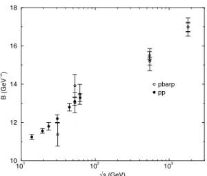
that the mathematical description of the increase of the total cross sections at the highest energies is an open problem. As we shall discuss, the study of the effects of the discrepant points at the highest energies is one of our goals. Fig. 2 shows the typical diffractive pattern that characterizes the differential cross section. We note that the data cover the region corresponding to 10 decades. In Fig. 3 it is displayed the slope parameter fromppandpp¯ scattering as function of the energy and determined in the region of small momentum transfer. In what follows we shall refer to these three figures as indicative of the empirical behavior of the quantities in-volved.
101 102 103 104 105
√s (GeV)
30 60 90 120 150 180 210
σtot
(mb)
Akeno Fly’s Eye Nikolaev GSY accelerator pp accelerator p(bar)p
Figure 1. Total cross sections onppandpp¯ from accelerator and cosmic-ray experiments (for complete list of references and tables see [10]).
0.0 2.0 4.0 6.0 8.0 10.0
|t| (GeV2) 10−10
10−8 10−6 10−4 10−2 100 102
d
σ
/dt (mb/GeV
2)
101 102 103
√s (GeV) 10
12 14 16 18
B (GeV
−2)
pbarp pp
Figure 3. The slope parameter as function of the energy and deter-mined in the interval 0.01<|t|<0.20 GeV2.
2.2
Principles,
theorems and high-energy
bounds
For our purposes, we recall some principles and theorems from axiomatic quantum field theories [11]. The basic Prin-ciples are: Lorentz Invariance, Unitarity (related with the conservation of probability), Analyticity (related to causal-ity) and Crossing (connecting particle and particle-antiparticle interactions). Analyticity and crossing allow the connections between real and imaginary parts of the scatter-ing amplitude by means of dispersion relations.
Several rigorous theorems and bounds may be deduced from the basic Principles and axiomatic quantum field the-ory. Among them, the Froissart-Martin bound concerns the increase of the total cross section stating that
σtot≤Clog2
s
s0 as s→ ∞. (5)
The Pomeranchuk Theorem treats the difference be-tween cross sections for particle (ab) and particle-antiparticle scattering (a¯b). The original form was deduced when it was believed that the cross section decreased to a constant value, and in this caseσab
tot=σtotab ass→ ∞.
Af-ter the discovery of the rising of the cross section, Grunberg and Truong obtained the generalized or revised form of the Pomeranchuk Theorem, stating that
σab tot−σa
¯
b tot
σab tot+σa
¯
b tot
→0 or σ ab tot
σab tot
→1 as s→ ∞,
and this means that, if the Froissart-Martin bound is reached, then
∆σ≡σab
tot−σabtot≤C
σab tot+σtotab
logs ≤Clogs. (6)
By expressing the cross sections in terms of crossing even (+) and odd (−) contributions,
σ±(s) =
σab tot±σa
¯
b tot
2 ,
we have |∆σ| = |σabtot −σtotab| = 2σ− . Therefore,
∆σ ≡ σab
tot −σabtot → 0 if and only if σ− → 0. This
possible odd contribution is named Odderon and the case of even dominance at asymptotic energies is associated with the Pomeron.
2.3
Basic pictures
Nearly all the phenomenological models, able to describe the experimental data on elastic hadron scattering, are based on the Optical/Geometrical Picture (s-channel) and/or the Exchange Picture (t-channel). The corresponding formulas may be obtained from the Partial Waves representation of the scattering amplitude,
F(k, θ) = i 2k
∞
l=0
(2l+ 1)
1−e2iδlP
l(cosθ),
whereδlis the phase shift. In what follows, we outline the
main steps and formulas in both pictures.
2.3.1 Optical/Geometrical Picture
From the partial wave representation, one considers the high-energy limit and the semi-classical approximation, so that the discrete angular momentuml may be replaced by the continuum impact parameterb,
l=kb−12.
In turn, the discrete phase shiftsδlare replaced by the
con-tinuum eikonal function ofbands,χ(s, b)and
∞
l=0 ... →
∞
0 db...
The scattering amplitude in thisEikonal Representation, with azimuthal symmetry assumed, reads
F(s, q) =ik
∞
0
bdbJ0(qb)[1−eiχ(s,b)]. (7) The quantity
1−eiχ(s,b)≡Γ(s, b) (8) is named Profile function. From Unitarity this function is related to the probability that an inelastic event takes place atbands, the Inelastic Overlap function:
Since in the Eikonal representation
Ginel(s, b) = 1−e−2Imχ(s,b), (10)
forIm χ(s, b)≥0we haveGinel(s, b)≤1, which implies
in an automatically unitarized representation.
2.3.2 Exchange Picture
In this picture, from the partial wave representation, one considers the analytic continuation of the amplitude to com-plex angular momentum. In the asymptotic limit (s→ ∞) and with symmetry connecting the crossed channels one ar-rives at the Watson-Sommerfeld-Gribov-Regge representa-tion for the scattering amplitude, expressed as a sum over the poles of the amplitude (the Regge poles), as outlined in what follows.
As it is known at high energies the number of partial waves is large, and one way to circumvent that is to trans-form the sum of partial waves into a complex integral, and then use the residues theorem to obtain a new sum, but in-volving only the number of residues:
∞
l=0 ...→
C
g(l)dl→ N
m=0
Res g(l)|l=lm.
Detailed calculation allows one to obtain the following representation for the scattering amplitude,
F(k, θ) = N
i=1
βi(k)Pαi(k)(−cosθ)
sinπαi(k)
+BI(k, θ),
whereBI(k, θ)is called the Background integral. By con-sidering the high-energy limit (thenBI →0) and crossing (exchange four-momentap→ ⇔ ← −p) we can replace¯
the crossing channel variable (θ¯↔s)
cos ¯θ= 1−4m22s−t → ∝ −s as s→ ∞,
also,
Pl(x)→
2lΓ(l+ 1/2) √
πΓ(l+ 1)
xl for x→ ±∞,
and grouping all thes-independent quantities in a function
K(t)we have
Pα(t)(−cos ¯θ) =K(t)sα(t) for s→ ∞.
Rearranging the terms we arrive at a descending asymp-totic series in powers ofs, with leading contribution:
F(s, t) =γ(t)ξ(t)sα(t), (11)
whereγ(t)is the residue function,ξ(t)the signature factor andα(t) = α(0) +α′t the trajectory function. This last
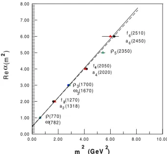
function connects the spin and masses through the Chew-Frautschi plot, as exemplified in Fig. 4. In this picture the interaction of the colliding particles is basically inter-preted in terms of exchanges of Regge poles (also Regge cuts) and the Pomeron (anad hoctrajectory with intercept nearly above 1). We note that, as constructed, the exchange picture is intended for asymptotic energies.
0 .0 0 2 .0 0 4 .0 0 6 .0 0 8 .0 0 1 0 .0 0 0 .0 0
1 .0 0 2 .0 0 3 .0 0 4 .0 0 5 .0 0 6 .0 0 7 .0 0 8 .0 0
m2 (G eV )2
Re
(
m
)
α
2
f (1 2 7 0 )2
4
f (2 0 5 0 )
f (2 5 1 0 )6 a (2 4 5 0 )6
a (2 0 2 0 ) 4
a (1 3 1 8 )2
(2 3 5 0 ) ρ5
(1 7 0 0 ) ρ3
(1 6 7 0 ) ω3
(7 7 0 ) ρ
(7 8 2 ) ω
Figure 4. The Chew-Frautschi plot for some mesons and reso-nances.
3
Analytic approach
The Analytic Approach for elastic hadron-hadron scattering is based on general principles and theorems from Quantum Field Theory. It is characterized by analytical parametriza-tions for the imaginary part of the forward amplitude, to-gether with the use of dispersion relation techniques. The central point is the simultaneous investigation of the total cross section (imaginary part of the scattering amplitude, Eq. (2)) and theρparameter (connected with the real part of the amplitude, Eq. (3)).
For particle-particle and particle-antiparticle interac-tions, dispersion relations are consequences of the principles of Analyticity and Crossing. In this context, they correlate real and imaginary parts of crossing even (+) and odd (−) amplitudes, which in turn are expressed in terms of the scat-tering amplitudes for a given process and its crossed chan-nel, for example,a+banda+ ¯b:
Fab=F++F−, Fa¯b =F+−F−. (12)
ReF+(s) =K+2s
2
π P
+∞
s0
ds′ 1
s′(s′2−s2)ImF+(s
′)
(13) and
ReF−(s) =
2s πP
+∞
s0
ds′ 1
(s′2−s2)ImF−(s
′), (14)
whereKis the subtraction constant and, forppandpp¯ scat-tering,s0= 2m2∼1.8GeV2.
In this section we review some results obtained through this approach. We start with the replacement of the above in-tegral forms by derivative operators (Derivative Dispersion Relations) and then we discuss the use of analytic models (Reggeons, Pomeron, Odderon) for parametrizations involv-ing the total cross section and theρ parameter, the deter-mination of bounds for the soft Pomeron intercept, and the practical role of the subtraction constant.
In what follows we are mainly concerned with theppand
¯
ppelastic scattering, since for particle and antiparticle inter-actions they correspond to the highest energy interval with available data and are the only set including the cosmic-ray information on total cross sections (ppscattering). As com-mented before, the experimental data available on the total cross sections (Figure 1) are characterized by discrepant ex-perimental information at the highest energies, and one of our aims is to investigate the effects of these discrepancies in the context of the analytic models. This concern perme-ates all the discussion in this Section.
3.1
Derivative Dispertion Relations
The use of dispersion relations in the investigation of scat-tering amplitudes may be traced back to the end of fifties, when they were introduced in the form ofIntegral Disper-sion Relations (IDR). Despite the important results that have been obtained since then, one limitation of the integral forms is their non-local character: in order to obtain the real part of the amplitude, the imaginary part must be known for all values of the energy. Moreover, the class of functions that allows analytical integration is limited.
In the last years, we have investigated the applicability of DerivativeDispersion Relations (DDR) in place of integral forms [12, 13, 14, 10, 15, 16]. In Reference [16] we present a recent review on different results and statements related to this replacement, and a discussion connecting these differ-ent aspects with the corresponding assumptions and classes of functions considered in each case.
In particular, we have shown that for the class of func-tions which are entire in the logarithm of the energy (as is the case of analytic models at high energies) it is possi-ble to expand the integrand in the above formulas and by considering a high-energy approximation, represented by s0 = 2m2 → 0, to integrate term by term. In that case, as demonstrated in detail in [16], the derivative dispersion relations with one subtraction reads
ReF+(s)
s =
K s + tan
π
2 d d ln s
ImF+
(s)
s , (15)
ReF−(s)
s = tan
π
2
1 + d
d ln s
ImF−(s)
s , (16) where the series expansion is implicit in the tangent opera-tor. From this deduction one arrives to three formal results: (1) the subtraction constant is preserved when the IDR are replaced by DDR and, therefore, in principle, can not be disregarded in fit procedures; (2) except for the subtraction constant, the DDR with entire functions in the logarithm of the energy do not depend on any additional free para-meter; (3) the only approximation involved in the replace-ment concerns the lower limit in the IDR (13-14), namely s0= 2m2→0, which represents a high-energy approxima-tion. In the next two subsections we discuss some uses of the DDR with analytical models, and in the third subsection we return to the replacement of IDR by DDR, investigating the important role of the subtraction constant from a practical point of view.
3.2
Basic Models
In this Subsection we make use of two basic and well known parametrizations for the total cross sections and investigate the effects of the discrepancies in the experimental informa-tion from cosmic-ray experiments.
3.2.1 Ensembles
In the cosmic-ray region,6TeV<√s≤ 40TeV, the dis-crepancies on the total cross section information are due to both experimental and theoretical uncertainties in the deter-mination ofσtotpp from p-air cross sections. The situation has
been recently reviewed in detail in [10], where a complete list of references, numerical tables and discussions are pre-sented.
From Fig. 1 we see that, despite the large error bars in the cosmic-ray region, we can identify two distinct sets of esti-mations: one corresponding to the results by the Fly’s Eye Collaboration (Fly’s Eye) together with those by the Akeno Collaboration (Akeno); the other set associated with the re-sults by Gaisser, Sukhatme, and Yodh (GSY) together with with those by Nikolaev (Nikolaev). Taken separately these two sets suggest different scenarios for the increase of the total cross section, as previously discussed in [13, 17, 18].
Based on these considerations, it is important to inves-tigate the behavior of the total cross section by taking into account the discrepancies that characterize the cosmic ray information. To this end, in [10] we have considered two ensembles of data and experimental information, as follows:
• Ensemble I: pp¯ and pp accelerator data + Akeno + Fly’s Eye;
To some extent, ensemble I represents a kind of high-energy standard picture and ensemble II a nonstandard one.
3.2.2 Analytic Models
With analytical parametrizations for pp/pp¯ total cross sec-tions, the connections with the ρparameter, Eq. (3), are obtained by defining the associated crossing even and odd quantities,
σ±(s) =σ
pp tot±σ
¯
pp tot
2 , (17)
using the high-energy normalization for the Optical Theo-rem,
σtot(s)∼
ImF(s,0)
s , (18)
and the DDR given by Eqs. (15) and (16).
In [10] we have considered two different parametriza-tions for the total cross secparametriza-tions, one introduced by Don-nachie and Landshoff [19] and other by Kang and Nicolescu [20]. The main difference concerns the asymptotic limits, which allow the dominance of an even amplitude (Pomeron) or the odd amplitude (Odderon), respectively. In this way, we may contrast these possibilities with the standard and non-standard pictures represented by Ensembles I and II.
TheDonnachie-Landshoff (DL) parametrization for the total cross sections is expressed by
σpptot(s) =Xsǫ+Y s−η, σ
¯
pp
tot(s) =Xsǫ+Zs−η, (19)
where the first contribution is associated with a single Pomeron exchange (universal) and the second one with Reggeon exchange. With the procedure explained above, we obtain the analytical connections with the ρparameter forppandpp¯ scattering:
ρpp(s)σpptot(s) =
K s +
Xtanπǫ 2
sǫ
+ (Y
−Z)
2 cot
πη
2
−(Y +Z)
2 tan
πη
2
s−η,
ρpp(s)σpptot(s) =
K s +
Xtanπǫ 2
sǫ
+ (Z
−Y)
2 cot
πη
2
−(Y +2 Z)tanπη 2
s−η.
From the above formulas, sinceη > 0, this model pre-dicts that, asymptotically (s→ ∞),
∆σ = σtotpp(s)−σ pp
tot(s)→0, ∆ρ = ρpp¯ (s)−ρpp(s)→0.
The parametrization for the total cross sections intro-duced byKang and Nicolescu(KN), under the hypothesis of the Odderon, is given by
σtotpp(s) =A1+B1lns+kln2s,
σtotpp(s) =A2+B2lns+kln2s+ 2R s1/2, and the connections withρread
ρpp(s)σtotpp(s) =
K s +
π
2
B1+B2
2
+
πk+A2−A1
π lns+
B2
−B1
2π ln
2
s−s21R/2,
ρpp(s)σtotpp(s) =
K s +
π
2
B1+B2
2
+
πk−A2−πA1 lns−
B2−B1
2π ln
2 s.
Differently from the previous case, this model predicts that the difference between the two cross sections is given by
∆σ = (A2−A1) + (B2−B1) lns+ 2Rs−1/2
→ ∆A+ ∆Blns (asymptotically),
so that, if∆A = 0and/or∆B = 0, the total cross section difference may increase andσtotpp may even become greater
thanσpptot¯ , depending on the values and signs of ∆A and ∆B, which is formally in agreement with the theorems of Sec. 2.B. Moreover, if∆Aand∆B are sufficiently small, so that we may replaceσtotpp¯ ≈σ
pp
tot≡σtot(s), then,
asymp-totically,
∆ρ=ρpp−ρpp∼ − 1
πσtot(s)
∆Alns+ ∆Bln2s
.
This means that, depending on the fit results, there may be a change of sign in∆ρ, withρppbecoming greater thanρpp
at some finite energy. Therefore, the case of a crossing ei-ther inσtotorρis a sign of the odderon contribution in the
imaginary or real part of the amplitude, respectively.
3.2.3 Fits and Results
We have performed 16 different fits through the program CERN-MINUIT. In these fits we have used both ensembles I and II and both the DL and KN models. For each of these four possibilities we have performed global and individual fits toσtotandρand, in each case, we either considered the
subtraction constantK as a free fit parameter, or assumed K= 0.
Despite the small influence from different cosmic-ray esti-mations, the results allow to extract an upper bound for the soft Pomeron intercept:1 +ǫ= 1.094; (2) although global fits present good statistical results, in general, this procedure constraints the rise ofσtot; (3) the subtraction constant as a
free parameter affects the fit results at both low and high en-ergies; (4) independently of the cosmic-ray information used and the subtraction constant, global fits with the Odderon parametrization predict that, above√s ≈ 70 GeV,ρpp(s)
becomes greater thanρ¯pp(s), and this result is in complete
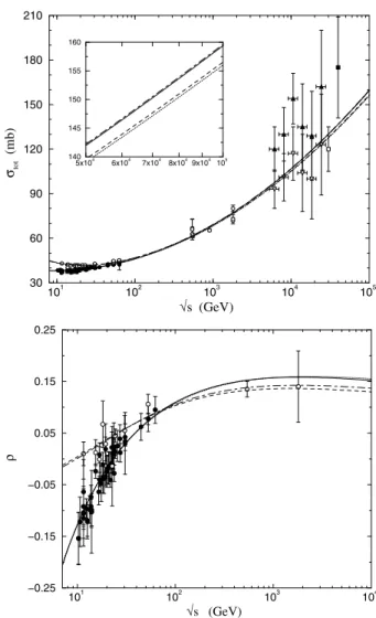
agreement with all the data presently available. That result is displayed in Fig. 5 and we can inferρpp= 0.134±0.005
at√s = 200GeV and0.151 ± 0.007at500GeV (BNL RHIC energies).
101 102 103 104 105
√s (GeV)
30 60 90 120 150 180 210
σtot
(mb) 5x10⁴ 6x10⁴
7x10⁴ 8x10⁴
9x10⁴ 105 140
145 150 155 160
101
102
103
104
√s (GeV)
−0.25 −0.15 −0.05 0.05 0.15 0.25
ρ
Figure 5. Simultaneous fits toσtot(s)andρ(s)through the KN
parametrization withK= 0and ensembles I (dotted curves forpp and dashed forpp¯) and II (solid curves forppand dot-dashed for
¯
pp) [10].
3.3
Non-degenerate Meson Trajectories
The DL parametrization referred above assumes degenera-cies between the secondary reggeons, imposing a common intercept for theC= +1(a2, f2) and theC=−1(ω, ρ) tra-jectories (see Fig. 4). More recently, analysis treating global
fits toσtotandρhave indicated that the best results are
ob-tained with non-degenerate meson trajectories. In this case the forward scattering amplitude is decomposed into three reggeon exchanges,F(s) =FIP(s)+Fa2/f2(s)+τ Fω/ρ(s), where the first term represents the exchange of a single soft Pomeron, the other two the secondary Reggeons and
τ = +1(−1) forpp (pp¯ ) amplitudes. Using the notation
αIP(0) = 1 +ǫ,α+(0) = 1−η+andα−(0) = 1−η− for
the intercepts of the Pomeron and theC= +1andC=−1
trajectories, respectively, the total cross sections, Eq. (18), forppandpp¯ interactions are written as
σtot(s) =Xsǫ+Y+s−η++τ Y−s−η− (20)
and the connection with theρparameter by means of DDR is similar to that displayed in the last subsection.
Making use of this parametrization, in this section we present the determination of extrema bounds for the Pomeron intercept [15] and a practical analysis on the re-placement of IDR by DDR together with a discussion on the role of the subtraction constant [16].
3.3.1 Extrema Bounds for the Pomeron Intercept
In order to analyze the extrema effects in the soft Pomeron intercept due to discrepancies in the experimental data, we performed a detailed analysis including the highest and the lowest values of the total cross section from both accelera-tors and cosmic-ray experiments.
As it is well known, in the accelerator region, the con-flict concerns the results forσpptot¯ at√s= 1.8TeV reported by the CDF Collaboration and those reported by the E710 and the E811 Collaborations (Fig. 1). In the cosmic-ray re-gion, as we have discussed, the highest predictions forσtotpp
concern the result by Gaisser, Sukhatme, and Yodh together with those by Nikolaev. In order to treat the lowest esti-mations in the cosmic-ray region, we consider the results obtained by Block, Halzen, and Stanev (BHS), by means of a QCD-inspired model. As discussed in [10], the reason for this choice is that, although the extractedσpptot(s)shows agreement with the Akeno results, it is about17mb below the Fly’s Eye value at30TeV and therefore may be consid-ered as a extreme lower estimate. All the numerical tables and references can be found in [10].
In this case we have considered the following ensembles of experimental information. First we only consider accel-erator data in two ensembles with the following notation:
•Ensemble I:σtotpp andσtotpp¯ data (10≤√s≤900GeV) + CDF datum (√s= 1.8TeV);
•Ensemble II : σtotpp andσtotpp¯ data (10 ≤ √s ≤ 900
GeV) + E710/E811 data (√s= 1.8TeV).
Ensemble I represents the faster increase scenario for the rise of σtot from accelerator data and ensemble II the
(BHS) results, respectively. These new ensembles are de-noted by
•I + NGSY
•II + BHS
As in the previous analysis, we have considered both in-dividual fits toσtot, and simultaneous fits toσtotandρ,
ei-ther in the case where the subtraction constant is considered as a free fit parameter or assumingK= 0.
From this analysis, in the case of only accelerator data, we could infer the following upper and lower values for the Pomeron intercept: αIP(0) = 1.098±0.004(global fits to
ensemble I, withK = 0) andαIP(0) = 1.085±0.004
(in-dividual fit to σtot from ensemble II), with bounds 1.102
and 1.081, respectively. Adding the cosmic-ray informa-tion, we inferred the following upper and lower values: αIP(0) = 1.104±0.005(individual fit toσtotfrom
ensem-ble I + NGSY) andαIP(0) = 1.085±0.003(global fits to
ensemble II + BHS andKas a free fit parameter or individ-ual fit to σtot from this ensemble), with bounds1.109and 1.082, respectively. Therefore we may infer the following extremabounds for the soft Pomeron intercept:
αupperIP (0) = 1.109, αlowerIP (0) = 1.081.
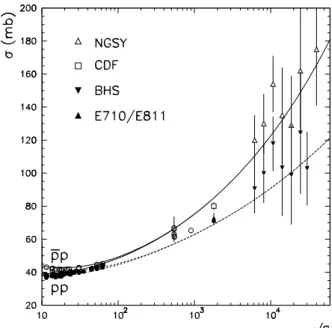
Figure 6 shows the total cross sections with parametrization (20) and the above extrema bounds, together with the exper-imental information available.
Figure 6. Fastest and slowest increase scenarios for the rise of the total cross section through parametrization (20) and allowed by the experimental information available: fits to ensembles I + NGSY (solid) and II (dashed) [21].
Extensions of theseextrema boundsfor the pomeron in-tercept to meson-p, gamma-p and gamma-gamma scattering have been discussed in [21]. By means of global fits to total cross section data it is shown that these bounds are in agree-ment with the bulk of experiagree-mental data presently available,
and extrapolations to higher energies indicate different be-haviors for the rise of the total cross sections.
We have also obtained newconstrained boundsfor the Pomeron intercept from spectroscopy data (Chew-Frautschi plots) and have extended the analysis to baryon-p, meson-p, baryon-n, meson-n, gamma-p and gamma-gamma scatter-ing [22]. It is also presented tests on factorization and quark counting rules with both extrema and constrained bounds (asymptotic energy region). In particular, at 14 TeV (CERN LHC) the extrema and constrained bounds allow to infer σtot= 114±25mb and105±10mb, respectively. [22].
3.3.2 IDR, DDR and the Subtraction Constant
As commented before, we have shown in Ref. [16] that for entire functions in the logarithm of the energy the only ap-proximation involved in the replacement of IDR by DDR concerns the lower limit s0 in the IDR: the high-energy condition is reached by assuming thats0 = 2m2 → 0 in Eqs. (13-14). In that paper we have investigated the practi-cal applicability of the DDR and IDR in the context of the Pomeron-reggeon parametrizations, with both degenerate and non-degenerate higher meson trajectories. By means of global fits toσtot(s)andρ(s)data fromppandpp¯ scattering,
we have tested all the 16 important variants that could affect the fit results, namely the number of secondary reggeons, energy cutoff (5 and 10 GeV), effects of the high-energy approximation connected with the subtraction constant and the analytic approach using both DDR and IDR with fixed s0. Our results led to the conclusion that the high-energy ap-proximation and the subtraction constant affect the fit results at both low and high energies. This effect is a consequence of the fit procedure, associated with the strong correlation among the free parameters.
A striking novel result concerns the practical role of the subtraction constant. We have shown that, with the Pomeron-reggeon parametrizations, once the subtraction constant is used as a free fit parameter, the results obtained with the DDR and with the IDR (with finite lower limit, s0 = 2m2) are the same up to 3 significant figures in the fit parameters andχ2/DOF. This conclusion, as we have shown, is independent of the number of secondary reggeons (DL or extended parametrization) or the energy cutoff (√s = 5 or 10 GeV). In Table 1 we display the fit results with the extended parametrization and cutoff at 10 GeV.
4
Model Independent Analysis
TABLE 1. Simultaneous fits toσtot andρthrough the extended parametrization,√smin =10 GeV (154 data points), withKas
a free parameter and using IDR with lower limits0 = 2m2 and
DDR [16].
IDR withs0= 2m2 DDR
X 19.57±0.79 19.58±0.78
Y+ 66.0±6.7 66.0±6.6
Y− -29.2±4.0 -29.2±4.0
ǫ 0.0897±0.0033 0.0897±0.0033 η+ 0.380±0.033 0.380±0.033
η− 0.520±0.025 0.520±0.024
K -14±48 104±58
χ2
/DOF 1.10 1.10
4.1
Differential Cross Section
Several authors have investigated elastic hadron scattering by means of parametrizations for the scattering amplitude and fits to the differential cross section data, Eq. (1). The extraction of the Profile, Eikonal and Inelastic Overlap func-tions in theb-space (impact parameter) and, in some special cases, the Eikonal in theq2-space, has led to important and novel results related with geometrical aspects (radius, cen-tral opacity), differences between charge distributions and hadronic matter distributions, existence or not of eikonal zeros in theq2-space and, more recently, connections with pomerons, reggeons and nonperturbative QCD aspects. In Ref. [23] we present a review and a critical discussion on the main results concerning this kind of analysis and also a wide list of references to outstanding works.
The basic input in all these analyses is the parametriza-tion of the scattering amplitude as a sum of exponentials in q2(as empirically suggested by the diffractive pattern shown in Fig. 2) and fits to the differential cross section data. This parametrization allows analytical expressions for the Fourier transform of the amplitude, providing also analytical expres-sions for the quantities of interest in theb-space.
In the next two subsections we review the results we have obtained by means of unconstrained fits (fit parameters completely free, without extracted dependences on the en-ergy) [23, 24], and discuss some research in course related to constrained fits (including dependences on the energy which are based on empirical information) [27].
4.1.1 Unconstrained Fits and the Eikonal
In the high energy region,√s >10 GeV, differential cross section data are available at √s =13.8, 19.5, 23.5, 30.7, 44.7, 52.8 and 62.5 GeV forppscattering and at√s=13.8, 19.4, 31, 53, 62, 546 and 1800 GeV forpp¯ scattering. Data frompp scattering also exists at√s =27.5 GeV and 5.5
≤q2≤14.2 GeV2(but not onσ
totandρ), and as we shall
show, that set plays a fundamental role in our analyse. See [23] for a complete list of references.
As discussed in [23] two main problems are typical of model independent analysis of the differential cross sec-tions:
(1) Experimental data are available only over finite re-gions of the momentum transfer (which in general are small, q2 <7 GeV2) and the Fourier transform demands integra-tion fromq2= 0 to infinity. This means that any fit is biased by extrapolations and although some extrapolated curves may look unphysical, they can not be excluded on mathe-matical grounds.
(2) The exponential parametrization allows analytical determination of the quantities in the b-space (profile, in-elastic, eikonal functions) and also the statistical uncertain-ties, by means of error propagation from the fit parameters. However, in this case, the translation of the eikonal from b-space to theq2-space can not be analytically performed and neither the error propagation (through standard procedures). As a consequence, the unavoidable uncertainties from the fit extrapolations can not, in principle, be taken into account.
In what follows we review a model independent ap-proach able to minimize the above two problems.
-Fit Procedure
In order to treat problem (1) we have used the follow-ing procedure [24]. Since it is known that for larget the experimental data do not depend on the energy at13.8GeV
≤ √s ≤ 62GeV and that there exist data at√s = 27.5
GeV in the region5.5GeV2 ≤q2 ≤14.2GeV2, we have selected two ensembles ofppandpp¯ differential cross sec-tion data:
•Ensemble I: experimental data at each energy;
•Ensemble II: Ensemble I + data at√s= 27.5GeV. For the scattering amplitude we have introduced the following model independent analytical parametrization for both real and imaginary parts:
F(s, q) ={µ 2
j=1
αje−βjq
2
}+i{ n
j=1
αje−βjq
2
}, (21)
µ= ρ(s)
α1+α2
n
j=1
αj. (22)
With the experimental ρ value at each energy the fits to the differential cross section data have been performed through the CERN-MINUIT routine and the validity or not of ensemble II is checked by means of the MINUIT output and standard statistical interpretation of the fit results (DOF, confidence levels).
Forppscattering we have found that the data at√s =
13.8 GeV are not compatible with ensemble II. In the case of pp¯ scattering none of the data sets are compatible with ensemble II. Therefore, in what follows, ensemble II (data at√s=27.5 GeV added) corresponds only toppscattering at 6 energies: 19.5, 23.5, 30.7, 44.7, 52.8 and 62.5 GeV.
From the error matrix (variances and covariances), χ2/DOF and confidence intervals, we infer the best values for the parameters and corresponding errors∆αj,∆βj. By
means of standard error propagation, the uncertainties in the free parameters,∆αj,∆βj, (j= 1, 2, ...) have been
dσ dq2 ±∆
dσ
dq2 . (23)
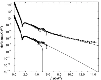
By adding and subtracting the corresponding uncertainties we may estimate the confidence region associated with all the extrapolations, which cannot be excluded on statistical grounds. A typical result with ensembles I and II is illus-trated in Fig. 7, forppscattering at√s= 23.5 GeV. We see that, as expected, the effect of adding the experimental data at√s= 27.5 GeV (when statistically justified) is to reduce drastically the uncertainty region. That result will be funda-mental in the extraction of the empirical information on the eikonal, as shown in what follows.
0.0 2.0 4.0 6.0 8.0 10.0 12.0 14.0
q2 (GeV2)
10−15 10−13 10−11 10−9 10−7 10−5 10−3 10−1 101 103 105
d
σ
/dt (mb/GeV
2 )
Figure 7. Regions of uncertainties (limited by the solid lines) in fits toppdifferential cross section data, Eq. (23), at√s= 23.5GeV with ensembles I (below) and II (above) [23].
- Eikonal in the momentum transfer space
By means of the Fourier transform, Eqs.(7-8), the para-metrization (21-22) provides analytical expressions for the real and imaginary parts of the Profile function,ΓR(s, b)and ΓI(s, b), and also the associated uncertainties. From the fit
results, together with error propagation, we have found that
Γ2I(s, b) [1−ΓR(s, b)]2 ≪
1,
and therefore, the imaginary part of the eikonal may be ap-proximated by
χI(s, b)≈ln 1 1−ΓR(s, b)
(24) and the uncertainty ∆χI determined directly from ∆ΓR
through propagation.
The next step is to go to the momentum transfer space and concerns problem (2): the Fourier transform can not be performed analytically and therefore also the error propa-gation. For this reason we used a semi-analytical method
as follows. Expanding the above equation, we express the remainder of the series as
R(s, b) = ln[ 1 1−ΓR(s, b)
]−ΓR(s, b) (25)
and then fit the numerical points (MINUIT) by a sum of Gaussians in the impact parameter space:
Rfit(s, b) =
6
j=1
Aje−Bjb
2
. (26)
A typical result is displayed in Fig. 8.
0 0.5 1 1.5 2
b (fm)
0 0.2 0.4 0.6
R(s,b)
0.8 1 1.2
b (fm)
0 0.05 0.1
R(s,b)
Figure 8. Typical parametrization for the generated remainder R(s, b)by means of Eq. (26) [23].
With this, the errors∆Ajand∆Bj may be propagated
determining∆Rf it(s, q)and thenχI(s, q)±∆χI(s, q). In
order to check the results and approximations, we performed also numerical integration through the NAG routine. -Results
One of the main results extracted from this analysis is the statistical evidence of eikonal zeros in the momentum transfer space, first presented in [24]. In order to investigate the position of the zeros and, mainly, to determine the un-certainties in its values, we consider the expected behavior ofχI at largeq2, namelyχI ∼q−8. In Fig. (9) we show a
typical plot of the quantityq8χ
I(s, q)as function ofq2. The
0.0 4.0 8.0 12.0 16.0 20.0
|t| (GeV2 )
-0.5 0.0 0.5 1.0
t
4χ
I
(GeV
6)
-0.5 0.0 0.5 1.0
(a)
0.0 4.0 8.0 12.0 16.0 20.0
|t| (GeV2)
-0.5 0.0 0.5 1.0 1.5
t
4χ
I
(GeV
6)
(a)
Figure 9. The eikonal in the transfer momentum space (multiplied byt4
) forppat√s= 30.7GeV with ensemble I (above) and II (below) [23].
From plots like that we can determine the positions of the zeros and the associated errors from the extrems of the uncertainty region (in general not symmetrical). The po-sition of the zero can also be obtained from the numerical method, but without uncertainties.
In Figure 10 it is shown the position of the zeros as function of the energy determined by means of both the semi-analytical (with uncertainties) and numerical (without uncertainties) methods. Despite the systematic difference on the values with these methods, we may conclude that the position of the zero decreases as the energy increases. Roughly,q2
0: 8.5→6.0GeV2as√s: 20→60GeV.
20 30 40 50 60 70
s1/2 (GeV)
5 7 9 11
q
2 (GeV0 2 )
semi−analytical numerical
Figure 10. Position of the eikonal zero in the momentum transfer space as function of the energy [23].
-Discussion
As reviewed in [23], there has been previous indica-tion of eikonal zeros in the momentum transfer space, but without associated uncertainties. Our first statistical evi-dence, published in 1997, indicated the position of the zero atq2
0= 7±2GeV2[24]. In 2000, experiments performed at the Jefferson Laboratory, on electron-proton scattering, have indicated an unexpected decrease of the ratio between the electric and magnetic proton form factors as the momentum transfer increases from 0.5 to 5.6 GeV2. Moreover, extrap-olations from empirical fits indicate a change of sign (zero) in this ratio, just atq2 ≈7.7 GeV2. Since forpp/pp¯ scatter-ing the eikonal is connected with the hadronic matter form factor (see Sec. 5, Eq. (38)), the above results on the po-sition of the zeros suggest novel and important insights on possible correlations between hadronic and electromagnetic interactions. We discuss that subject in [25], calling atten-tion to the possibility ofhadronic form factors depending on the energy.
We have also obtained the value of the imaginary part of the Eikonal at zero momentum transfer, that is, the central opacity. The results are displayed in Fig. 11. As discussed in [26], one naive way to test these results is with the Glauber model for the scattering involving hadronsAandB, and the Optical Theorem at the elementary level. In that case, the elementary cross section may be expressed by
σelem(s) =
4π
NANB
χI(s, q= 0),
whereNAandNBare the number of constituents in hadrons AandB, respectively. If we takeNA=NB = 3we obtain σelem ∼6mb at the ISR region, a result in agreement with
10 100 1000
s1/2 (GeV)
8 12 16 20 24 28
Im
χ
(s,q=0) (GeV
−2 )
p(bar)p pp
Figure 11. Imaginary part of the eikonal at zero momentum trans-fer, as function of the energy, from analysis onppandpp¯ scattering [23].
In Ref. [23] we discuss the applicability of our results in the phenomenological context, outlining some connections with nonperturbative QCD and presenting a critical review on the main results concerning “model-independent” analy-ses.
4.1.2 Constrained Fits and Energy Dependence
Despite the results obtained with the parametrization dis-cussed in the last subsection, due to the fit procedure, we do not have the dependence on the energy of the free parame-tersαi,βi. Presently, we are investigating that subject and
we review here some preliminary results [27].
The energy dependence has been introduced according to some empirical information: the increase of the total cross section and of the slope parameter withln2sandlns, re-spectively (see Figs 1 and 3). Let us consider the standard exponential parametrization for the imaginary part of the amplitude, normalized as
ImF(s, q2)
s =
n
i=1
αiexp[−βiq2]. (27)
Atq2= 0, from the optical theorem, Eq. (18), we expect a dependence of the parametersαiwithln2s, and the slope
represented by the parametersβi withlns. These are the
central choices in our approach. In order to treatppandpp¯
scatterings, in agreement with Analyticity and Crossing, we introduce crossing even and odd amplitudes and make use of the derivative dispersion relations, Eqs. (15) and (16), to connect real and imaginary parts of the amplitudes involved. Specifically, for the imaginary part of the scattering am-plitude we consider the parametrizations
ImFpp(s, q2)
s =
n
i=1
αi(s) exp[−βi(s)q2], (28)
ImF¯pp(s, q2)
s =
n
i=1
¯
αi(s) exp[−β¯i(s)q2], (29)
and, based on the above arguments, we introduce the follow-ing general dependences on the energy
αi(s) =Ai+Biln(s) +Ciln2(s)
βi(s) =Di+Eiln(s) (30)
forppscattering and
¯
αi(s) = ¯Ai+ ¯Biln(s) + ¯Ciln2(s) ¯
βi(s) = ¯Di+ ¯Eiln(s) (31)
forpp¯ scattering, wherei= 1,2, ...n. Defining the crossing even (+) and odd (-) amplitudes,
ImF+(s, q2) =ImFpp(s, q
2) + ImF¯
pp(s, q2)
2 , (32)
ImF−(s, q2) =
ImFpp(s, q2)−ImF¯pp(s, q2)
2 . (33)
the corresponding real parts can be determined by means of the leading terms of the DDR, Eqs. (15-16), and so the cor-responding real parts of the pp andpp¯ amplitudes. With these analytic amplitudes we obtain the differential cross section:
dσ dq2 =
1
16πs2|ReF(s, q
2) +iImF(s, q2)
|2. (34)
In order to treat simultaneous fits toppandpp¯ data we have considered only sets available at nearly the same en-ergy, namely√s ∼19.5, 31, 53 and 62 GeV. As a prelim-inary test we make use of data at the diffraction peak, out-side the Coulomb-nuclear interference region, 0.01 GeV2< q2≤0.5 GeV2, and the data providing the optical point,
dσ(s, q2= 0)
dq2 =
σtot(1 +ρ2)
16π . (35)
0.00 0.10 0.20 0.30 0.40 0.50 q2 (GeV2)
10−4 10−3 10−2 10−1 100 101 102
d
σ
/dq
2 (mb/GeV 2 )
(a)
19.5 GeV
30.7 GeV
52.8 GeV
62.5 GeV pp
0.00 0.10 0.20 0.30 0.40 0.50 q2 (GeV2)
10−4 10−3 10−2 10−1 100 101
102
d
σ
/dq
2 (mb/GeV 2 )
(b)
19.4 GeV
31.0 GeV
53.0 GeV
62.0 GeV pbarp
Figure 12. Differential cross section at the diffraction peak: fit re-sults and experimental data (displaced by a factor of 10) [27].
4.2
Total Cross Sections and Slopes
Another important quantity that characterizes the elastic hadron-hadron scattering is the slope parameter, defined in Eq. (4). In practice it may be determined by means of fits to the hadronic differential cross section data in the region of small momentum transfer, with the parametrization
dσ dt =
dσ
dt
t=0
e−B|t|, (36)
and, in general, it is connected with ρ and σtot through
fits in the region of Coulomb interference [2]. The slope and the total cross section are also important quantities in the determination ofσpptotfromσp−air (cosmic-ray
experi-ments) but, as commented before, the procedure is strongly model dependent. One reason is associated with the use of the Glauber multiple diffraction formalism, in whichσtot(s)
andB(s)take part in the parametrization of the elastic am-plitude,
Fpp(s, t)∝σpptot(s) exp
B(s)t
2
. (37)
As commented in [10] and [28], different models predict different relations betweenσtot(s)andB(s)and that is
mir-rored in the final value of the cross section, contributing to the discrepancies already discussed.
Based on the above observations, we have investigated the possibility to extract an empirical correlation between the experimental data onσtot(s)andB(s), fromppandpp¯
scatterings.
For the slope parameter, we have selected the data above the region of Coulomb-nuclear interference and below the “break” in the hadronic slope at the diffraction peak (local-ized at |t| ∼ 0.2 GeV2 at the ISR and Collider energies), namely 0.01<|t| <0.20 GeV2(Fig. (3)). In this region, the differential cross section data are well fitted by a single exponential and therefore there is no change in the slope as-sociated with the t-dependence. For each energy we have compiled the corresponding data on the total cross section.
Once more, the choice for a parametrization was based on the empirical observation that at high energiesB(s) in-creases with the logarithm ofs. Since the Kang-Nicolescu parametrization for the total cross section is expressed in terms oflns(Sec. 3.B.2), we replaced this dependence by the slope parameter:
σpptot(s) = c1+c2B+c3B2,
σpptot(s) = c1+c2B+c3B2+c4e−B/2, (38)
whereci, i = 1,2,3,4 are free fit parameters. That is a
strictly mathematical choice, having nothing to do with the physics or model concept behind the Kang-Nicolescu para-metrization.
Fits to the experimental data have been performed with the CERN-MINUIT program and the results are displayed in Fig. 13. It is expected that extrapolations to cosmic-ray energies may be useful in the determination of the pp to-tal cross section fromp-air cross section, allowing to con-nectσtot−Bin an almost model independent way. We are
presently investigating this subject.
In Ref. [28] we also made use of the Donnachie-Landshoff parametrization, which predicts a faster increase of the total cross section as function of the slope parameter. Moreover, in [28] we also present a critical discussion on the recent measurement of the slope parameter at the BNL RHIC, at 200 GeV, by the pp2pp Collaboration. We call attention to the fact that the combinationB =16.3 ±1.8 GeV−2andσtot =51.6 mb, indicated by the pp2pp
analy-sis, is in disagreement with the general trend for the behav-iors of σtot andB. If this “peer” is correct, new physics
is necessary. Using the aboveBvalue as input in our para-metrizations, the corresponding values of the total cross sec-tions show agreement with theσtotversusBdata. However,
these inferred values for σtot indicate new physics when
GeV2, a phenomenon that was never observed in both pp andpp¯ scattering, at√s ≤62.5 GeV and√s ≤1.8 TeV, respectively and therefore, once more, new physics is nec-essary.
10 12 14 16 18
B (GeV−2) 35
45 55 65 75 85
σtot
(mb)
pp ppbar pp ppbar
Figure 13. Total cross sections in terms of the slope, and the para-metrization (38) [28].
5
Eikonal Models
It is expected that the eikonal function in the momentum transfer space, χ(s, q), may be connected with some mi-croscopic aspects of the underlying field theory (elementary interactions, form factors, structure functions) and, as men-tioned before, it corresponds to a unitarized scheme con-nected with the experimental data. Eikonal models are char-acterized by different choices forχ(s, q). In what follows we discuss our results and researches through two eikonal models (geometrical and QCD-based)
5.1
Geometrical Model - Inelastic Channel
In this subsection we review the description of pp¯ multi-plicities distributions (inelastic channel) from models for the elastic channel in the context of the geometrical picture (contact interactions).
- Elastic and Inelastic Channels
Through the Unitarity and the Inelastic Overlap Func-tion, defined in Sec. 2.C, we can connect elastic and inelas-tic scattering. This is done by expressing the topological cross section for producting an even numbernof charged particles atsin terms ofGin:
σn(s) =
d2bσ
n(s, b) =
d2bG
in(s, b)
σ
n(s, b)
Gin(s, b)
.
If n(s) and < n >(s) are the hadronic and averaged multiplicities, respectively, by introducting the KNO vari-ableZ=n(s)/ < n >(s), the hadronic multiplicity distrib-ution may be expressed by
Φ(s, Z) =< n >(s) σn(s)
σin(s)=
d2bGin(b,s)
r(b,s) ϕ(r(Zb,s))
d2bGin(b, s) ,
where ϕ is the elementary multiplicity distribution and r(b, s) =< n >(b,s)/ < n >(s)the elementary multiplicity function.
In Ref. [29], in the context of the geometrical pic-ture, the elementary contact interaction process was based one+e−scattering data. In this approach we express
r(s, b) =ξ(s)χγI(s, b),
where
ξ(s) =
d2b G
in(s, b)
d2b G
in(s, b)χγI(s, b)
and the powerγis determined by fitting the average multi-plicity frome+e−scattering data through a power law
para-metrization:
< n >e+e−=A[
√
s]γ.
The elementary distributionϕ(Z/r(b, s))is represented by a Gamma distribution and determined also by fits to e+e−data.
With inputs forGin(s, b)and/orχI(s, b), obtained from
fits to elastic scattering data, we have no free parameter and the hadronic multiplicity distribution as function ofZands may be inferred.
- Elastic-channel inputs and results
In Ref. [29] we made use of three inputs from the elastic sector. Two are based on the Multiple Diffraction Formal-ism, in which the eikonal in the momentum transfer space is expressed by
χ(b, s) =C
qdqJ0(qb)GAGBf, (39)
whereGAandGB are the hadronic form factors,f the
el-ementary (constituent - constituent) amplitude andC does not depend on the transferred momentum. In this case we made use of the parametrizations used by Chou and Yang and also by Menon and Pimentel. Both present good de-scriptions of the experimental data in the elastic channel. The other input corresponds to the Short Range Expansion of the inelastic overlap function, introduced by Henzi and Valin,
Gin(b, s) =P(s) exp{−b2/4B(s)}k(x, s),
k(x, s) = N
n=0 δ2n(s)
ǫ exp{1/2}
2B(s) x 2n
.
With particular parametrizations excellent agreement with experimental data on pp and pp elastic scattering is achieved, allowing to infer the black-edge-large (BEL) be-havior.
In Ref. [29] a detailed discussion is presented on several variants from the elastic channel and parametrizations from e−e+scattering. In particular, the results for the multiplici-ties distributions, with the BEL inelastic overlap function, at
√
s=52.6 and 546 GeV are displayed in Fig. 14, together with the experimental data. The prediction shows that the violation of the KNO scaling is well described.
0.0 1.0 2.0 3.0 4.0
Z’=n’/<n’>
10-4 10-3 10-2 10-1 100 101
Φ(Ζ
’)
52.6 GeV
0.0 1.0 2.0 3.0 4.0
Z’=n’/<n’>
10-4 10-3 10-2 10-1 100 101
Φ(Ζ
’)
546 GeV
Figure 14. Scaled multiplicity distribution for inelasticppdata at
√s=
52.6 GeV andpp¯ data at 546 GeV, compared with the model predictions [29].
5.2
QCD-inspired models
In this section we outline some research in course with the eikonal approach in connection with some QCD concepts. As we shall discuss the main point concerns the gluon-gluon contributions to the hadronic cross sections which we have investigated either from a dynamical gluon mass approach or by introducting the momentum scale in the gluonic distri-bution functions. After a review on the basic formalism we outline some aspects of both approaches.
5.2.1 Basic formalism
The formalism was introduced by Afek, Leroy, Margolis and Valin [30] and developed by several authors, including (for our purposes) Durand, Pi [31], Block, Gregores, Halzen and Pancheri [32].
Originally, the point was to separate contributions from soft (S) and semi-hard (SH) inelastic processes by express-ing
Ginel(s, b) = 1−P¯SP¯SH
= 1−e−2Re χS(s,b)e−2Re χSH(s,b),
where P¯S is the probability of N O soft inelastic process
andP¯SHthe probability ofN Osemi-hard inelastic process.
Therefore, that indicated an additive contribution in the eikonal:χ(s, b) =χS(s, b) +χSH(s, b).
In the recent version by Block et al. [32] different el-ementary contributions from quarks and gluons have been introduced: the gluon-gluon contribution comes from the parton model, the quark-quark from regge parametrization and the quark-gluon by phenomenological inputs. In what follows we shortly review the main formulas.
The normalization for the eikonal reads
F(s, q) =ik
∞
0
bdbJ0(qb)1−eiχ(s,b),
χ(s, b) = Reχ(s, b) +iImχ(s, b).
Forppandpp¯ scattering the crossing even and odd con-tributions are expressed by χpp¯ = χ++χ− andχpp =
χ+−χ−. The odd eikonal is assumed not to contribute at
the asymptotic energies and is parametrized by
χ−(s, b) =C−m0√
se
iπ/4w(b, µ
odd).
Analyticity (generation of real and imaginary parts) for the even part is assumed as given by the prescription
χ+(s, b) ⇒ χ+(se−iπ/2, b) =
The even eikonal is expressed as a sum of three contri-butions, from quark-quark (qq), quark-gluon (qg) and gluon-gluon (gg) interactions,
χ+(s, b) =χ
qq(s, b) +χqg(s, b) +χgg(s, b),
which individually factorize insandb,
χij(s, b) =iσij(s)w(b, µij),
wherei, j=q, g.
The impact parameter distribution function for each process comes from convolution involving dipole form fac-tors (Chou-Yang Model):
wii(b, µii) =
d2b′ρi(|b′|ρi(|b−b′|),
ρ(b) =< G(q)>=< 1
(1 +q2/µ2)2 >,
where the angular brackets denote the symmetrical two-dimensional Fourier transform. Therefore,
wii(b) = 1 8
µ2
ii 12π[µiib]
3K3(µ
iib),
and fori=jit is assumed that
µij=√µiiµjj.
Theelementary cross sectionsfor each process are in-troduced as follows. Thequark-quarkcontribution is para-metrized as a constant plus a Regge (even) term,
σqq(s) =C+CR+
m0
√
s
and thequark-gluonterm as
σqg(s) =Cqglog
s s0.
The gluon-gluon contribution is considered as the re-sponsible for the increase of the total cross section at the highest energies and is calculated through the parton model approach,
σgg(s) =cgg
1
0
dτ Fgg(τ)ˆσgg(ˆs), (40)
with Fgg=
1
0
1
0
dx1dx2fg(x1)fg(x2)δ(τ−x1x2), (41)
wherefg(xi)is the gluon distribution function, τ = ˆs/s,
and the symbolˆdenotes the elementary process. In [32] the elementary cross section is given by
ˆ
σgg(ˆs) = 9πα2
s
m2 0
θ(ˆs−m20), (42)
implying a cutoffm0 for the particle production threshold and it is assumed the following simple parametrization for the gluon distribution function
fg(x) = Ng
(1−x)5 x1+ǫ ,
Ng = 1 2
(6−ǫ)(5−ǫ)...(1−ǫ)
5! . (43)
The model has 6 fixed parameters,m0,ǫ,µqq,µgg,µodd,
αs and 6 free parameters, determined from fits to ppand
pp¯forwardscattering data, namelyσtot(s),ρ(s)andB(s)
above 15 GeV [32]. We have shown that the model applies only to forward and small momentum transfer regions [33]. In the next two sections we shall discuss two researches in course concerning the determination of the contribution from gluon-gluon interactions, Eqs. (39-42).
5.2.2 Dynamical gluon mass
The possibility that the gluon propagator may be regular-ized by a dynamically generated gluon mass [34] has re-cently provided important phenomenological description of several processes [35]. The approach allows to calculate the contribution for the elementary ggcross section Eq. (42) and the main point is the association of the mass scale with the dynamical gluon mass. The basic ingredients are the ex-pressions for the dynamical gluon mass,
Mg2(ˆs) =m2g
ln[(ˆs+ 4mg2)/Λ2QCD]
ln[(4mg2)/Λ2QCD]
−12/11
,
and the associated running coupling constant
αs(ˆs) =
4π
β0ln(ˆs+ 4M2
g(ˆs))/Λ2QCD
,
whereβ0= 11−23nfandnf is the number of flavors. Pre-liminary tests with these contributions, in the context of the model described in the last subsection, have shown that the experimental data onσtot(s), ρ(s) andB(s)are well
Figure 15. Description of the total cross sections through the QCD-based model with dynamical gluon massm0 =500, 600 and 700
MeV [36].
5.2.3 Momentum Scale
Presently, we are attempting to improve the descriptions of the QCD-inspired models by taking into account the mo-mentum transfer scale in the gluon distribution functions. The point is to replace the simple choice in Eq. (42), by distribution functions with theQ2dependence, namely
fg(xi)→fg(xi, Q2).
That can be implemented, following the approach by Durand and Pi [31], by introducing the differential cross sec-tion
ˆ
σgg(ˆs) =
d|ˆt|dσˆgg
d|ˆt| (ˆs,ˆt),
with dσˆgg
d|ˆt|(ˆs,ˆt) = 9πα2
s 2 [
3 ˆ
s2 +
ˆ
t
ˆ
s3+
ˆ
t2
ˆ
s4 +
1 ˆ
t2 +
1 ˆ
sˆt
− ˆt
ˆ
s(ˆs+ ˆt)2]
and by consideringQ2=|ˆt|.
The novel input concerns the updated determinations of the gluon distribution functions (CETEQ6), parametrized by means of Chebyshev polynomials. Presently, the implemen-tation in the QCD-inspired approach is being developed.
6
Nonperturbative QCD
As commented before the difficulties associated with high-energy soft processes arise from the fact that perturbative
QCD can not be applied and presently we do not know how to calculate even the elastic hadron-hadron scattering ampli-tudes from a pure nonperturbative QCD formalism. How-ever, progresses have been achieved through the approach introduced by Landshoff and Nachtmann [37], developed by Nachtmann [38] and connected with the Stochastic Vacuum Model (SVM) (introductory reviews may be found in [39]). In particular, through this formalism and in some restricted kinematic conditions, it is possible to connect the gluon two-point correlation function with elementary (quark-quark) scattering amplitude.
In this section we review the results we have obtained for these amplitudes with correlators determined from lattice QCD and also in the context of the Constrained Instantons.
6.1
Stochastic Vacuum Model
The approach has its origins in the attempts by Landshoff and Nachtmann to connect soft high-energy processes with nonperturbative properties of the QCD vacuum, as for ex-ample, thegluon condensateintroduced by Shifman, Vain-stein and Zakharov [40]. In the first version [37] quarks couple with Abelian gluons. The non-Abelian version was developed by Nachtmann in the context of QCD and us-ing the eikonal method for high energy interactions [38]. The scattering amplitude is calculated by means of a func-tional integral approach and is connected to a correlation function of two lightlike Wegner-Wilson loops. These cor-relation functions can be evaluated through the Stochastic Vacuum Model, in which the low frequency contributions to the functional integral of QCD are described in terms of a stochastic process by means of a cluster expansion [41]. The model incorporates the gluon condensate concept and assumes that the correlation of two field strengths decreases rapidly with distance; due to an effective chromomagnetic monopole condensate, the QCD vacuum acts as a dual su-perconductor.
In this formalism the low frequencies contributions in the functional integral of QCD are described in terms of a stochastic process, by means of a cluster expansion. The most general form of the lowest cluster is the gauge invari-ant two-point field strength correlator [41, 42]
< FC
µν(x)FDρσ(y)>=
= δCDg2 < F F >
12(N2
c −1){
(δµρδνσ−δµσδνρ)κD(z2/a
2
) +
+ 1
2[∂µ(zρδνσ−zσδνρ) +
+ ∂ν(zσδµρ−zρδµσ)](1−κ)D1(z2/a
2
)},
wherez = x−y is the two-point distance,ais a charac-teristic correlation length, κa constant, g2 < F F >the gluon condensate and Nc the number of colours (C,D = 1, ..., N2
c −1). The two scalar functionsDandD1describe
constitutes important input for models aimed to construct hadronic amplitudes. The main formulas are as follows.
The elementary amplitudef in the momentum transfer space is expressed in terms of the elementary profileγby
f(q2) =
∞
0
bdbJ0(qb)γ(b). (44)
In the Nachtmann approach the no-colour exchange parton-parton (loop-loop) amplitude can be written as
γ = T r[Pe−ig
R
loop1dσµνFµν(x;w)
−1]
T r[Pe−ig
R
loop2dσρσFρσ(y;w)−1],
where means the functional integration over the gluon fields (the integrations are over the respective loop areas), andwis a common reference point from which the integra-tions are performed. In the SVM by taking the Wilson loops on the light-cone theleading ordercontribution to the am-plitude is given by
γ(b) =ηǫ2(b), (45) whereηis a constant depending on normalizations and
ǫ(b) =g2
dσµνdσρσT rFµν(x;w)Fρσ(y;w).
After a two-dimensional integration, ǫ(b) can be ex-pressed in terms of the correlation functions by
ǫ(b) =ǫI(b) +ǫII(b), (46)
where
ǫI(b) =κg2F F
∞
b
db′(b′−b)F2−1[D(k2)](b′), (47)
ǫII(b) = (1−κ)g2F FF2−1[ d dk2D1(k
2)](b).
(48) ForD=DorD=D1we haveD(k2) =F
4[D(z2)], where
Fndenotes a n-dimensional Fourier transform.
With the above formalism, once one has inputs for the correlation functionsD(z)andD1(z), the elementary am-plitude in the momentum transfer space, Eq. (43), may, in principle, be evaluated through Eqs. (44-47). It is im-portant to stress that, as constructed, the formalism is in-tended for small momentum transfer (q2 O(1) GeV2) and asymptotic energiess → ∞. Despite of these limita-tions, the investigation of soft high energy scattering at the energies presently available has led to satisfactory results [42, 43, 44].
6.2
Elementary Amplitudes
In this section we review the results we have obtained from inputs for the above correlators from lattice QCD [46, 47]. We also comment the research in course in the semi-classical context of Instantons [48].
6.2.1 Correlators from Lattice QCD
Numerical determinations of the above correlation func-tions, in limited interval of physical distances, exist from lattice QCD in both quenched approximation (absence of fermions) and full QCD (dynamical fermions included) [49].
With the procedure described above (see [46] for all the calculational details), the elementary scattering amplitude in the momentum transfer space can be determined in numer-ical form. In order to obtain analytnumer-ical expressions, suit-able for investigating distinct contributions and also for phe-nomenological uses, we have parametrized these numerical points through a sum of exponentials inq2:
f(q2) f(0) =
n
i=1
αie−βiq
2
. (49)
The results are displayed in Fig. (16) from both quenched approximation and full QCD, together with the correspond-ing exponential components.
0 2 4 6 8 10
q2 (GeV2) 10−1
100
f(q
2)/f(0)
quenched
0 2 4 6 8 10
q2 (GeV2) 10−1
100
f(q
2)/f(0)
full−QCD
Figure 16. Elementary amplitudes from quenched and full QCD and the exponential components through parametrization (48) [47].
![Figure 1. Total cross sections on pp and pp ¯ from accelerator and cosmic-ray experiments (for complete list of references and tables see [10])](https://thumb-eu.123doks.com/thumbv2/123dok_br/18981550.457210/2.892.518.811.397.642/figure-total-sections-accelerator-cosmic-experiments-complete-references.webp)
![TABLE 1. Simultaneous fits to σ tot and ρ through the extended parametrization, √ s min = 10 GeV (154 data points), with K as a free parameter and using IDR with lower limit s 0 = 2m 2 and DDR [16]](https://thumb-eu.123doks.com/thumbv2/123dok_br/18981550.457210/9.892.131.443.177.330/table-simultaneous-extended-parametrization-points-parameter-using-lower.webp)
![Figure 10. Position of the eikonal zero in the momentum transfer space as function of the energy [23].](https://thumb-eu.123doks.com/thumbv2/123dok_br/18981550.457210/11.892.142.414.62.727/figure-position-eikonal-momentum-transfer-space-function-energy.webp)
![Figure 11. Imaginary part of the eikonal at zero momentum trans- trans-fer, as function of the energy, from analysis on pp and pp¯ scattering [23].](https://thumb-eu.123doks.com/thumbv2/123dok_br/18981550.457210/12.892.98.440.80.368/figure-imaginary-eikonal-momentum-function-energy-analysis-scattering.webp)
![Figure 12. Differential cross section at the diffraction peak: fit re- re-sults and experimental data (displaced by a factor of 10) [27].](https://thumb-eu.123doks.com/thumbv2/123dok_br/18981550.457210/13.892.116.458.85.655/figure-differential-cross-section-diffraction-experimental-displaced-factor.webp)
