Nota Técnica
*e-mail: [email protected]
OPTIMIZATION AND PRACTICAL IMPLEMENTATION OF ULTRAFAST 2D NMR EXPERIMENTS
Luiz H. K. Queiroz Júnior*
Departamento de Química, Universidade Federal de São Carlos, Rod. Washington Luís, km 235, 13565-905 São Carlos – SP / Instituto de Química, Universidade Federal de Goiás, CP 131, 74001-970 Goiânia – GO, Brasil
Antonio G. Ferreira
Departamento de Química, Universidade Federal de São Carlos, Rod. Washington Luís, km 235, 13565-905 São Carlos – SP, Brasil Patrick Giraudeau
Université de Nantes, CNRS, Chimie et Interdisciplinarité: Synthèse, Analyse, Modélisation UMR 6230, B.P. 92208, 2 rue de la Houssinière, F-44322 Nantes Cedex 03, France
Recebido em 30/4/12; aceito em 17/10/12; publicado na web em 8/3/13
Ultrafast 2D NMR is a powerful methodology that allows recording of a 2D NMR spectrum in a fraction of second. However, due to the numerous non-conventional parameters involved in this methodology its implementation is no trivial task. Here, an optimized experimental protocol is carefully described to ensure efficient implementation of ultrafast NMR. The ultrafast spectra resulting from this implementation are presented based on the example of two widely used 2D NMR experiments, COSY and HSQC, obtained in 0.2 s and 41 s, respectively.
Keywords: ultrafast 2D NMR; COSY; HSQC.
INTRODUCTION
Analysis of the historical panorama of Nuclear Magnetic Resonance (NMR) reveals great evolution of this phenomenon1-3 since
the first records. Part of this impressive evolution is due the emergence of two-dimensional (2D)4,5 and imaging6,7 experiments. In spite of
this progress, conventional multidimensional NMR experiments still require a high number of scans to sample the indirect t1domain,
leading to long experiment durations (from several minutes to several hours). This limitation creates not only timetable constraints, but also renders conventional nD NMR experiments unsuitable for the study of kinetic or dynamic phenomena occurring on a short timescale or for hyphenated techniques such as LC-NMR. Several methodologies have been proposed to overcome this limitation in order to obtain spectra in shorter time frames,8-12 most notably the technique proposed by
Frydman et al.,13 also known as “ultrafast NMR” (UF-NMR). This technique allows performing of multidimensional experiments in a single scan, provided that sensitivity is sufficient.
The approach of UF-NMR differs to that used in its conven-tional counterpart, in terms of spin evolution and data acquisition. In a conventional 2D NMR experiment, spins are uniformly excited and t1 evolution is systematically incremented in a series of distinct
experiments. Acquisition is carried out by the storage of different FIDs (Free Induction Decays) from the corresponding incremented experiments.5 In the UF-NMR approach, the usual t
1 encoding is
re-placed by spatial encoding, and after a conventional mixing period, the spatially encoded information is decoded by a detection block based on echo planar imaging (EPI).7 The principles of UF-NMR have been
extensively described in recent reviews14-16 and are summarized below.
The spatial encoding scheme initially proposed by Frydman13,17
relies on a succession of frequency-selective pulses applied during alternating bipolar gradient pairs. However, it suffers from several drawbacks as it requires fast gradient switching, carefully synchro-nized with RF irradiation. Moreover, it leads to the appearance of undesirable ‘‘ghost peaks”18 in the indirect domain. Consequently,
this discrete excitation scheme was replaced by several continuous encoding patterns19-22 relying on the combination of continuous
fre-quency swept pulses applied during a bipolar gradient. The most ef-ficient approach in terms of resolution and sensitivity is probably that proposed by Pelupessy (Figure 1S, supplementary material),20 where
spatial encoding is carried out in a constant-time manner through the application of two chirp pulses concomitantly with a bipolar gradient pair (Ge). The first pulse/gradient combination results in quadratic
dephasing (z2) which requires the application of z² gradients for
re-focusing of the magnetizations arising from different z positions.An alternative consists of applying, following the first pulse, an identical pulse together with an opposite gradient. This leads to linear dephas-ing that depends linearly on position along the z axis and resonance frequency (W1). It should also be noted that in this excitation scheme,
spatial encoding is performed in a constant-time manner. Briefly, we can imagine the sample being divided into infinitesimal slices with dephasing varying linearly according to position.
The mixing step remains exactly the same as that used in con-ventional experiments,13,20 preserving the linear dephasing obtained
by the previous encoding block. For acquisition, a scheme based on echo planar imaging (EPI)7 is used. Firstly, after the receiver is open,
the acquisition gradient Ga (with duration of a few hundred
micro-seconds) is applied to refocus the dephasing acquired in the course of spatial encoding, leading to the formation of a series of echoes whose positions are proportional to the resonance frequencies that have been encoded (Figure 2S-a, supplementary material), where the signals observed during this period are similar to an 1D spectrum. As a consequence, the first dimension of the 2D spectrum, also called the “ultrafast dimension”, is obtained without any Fourier Transform. In order to obtain the second dimension, alternated ±Ga gradients
dimension, it is generally called a “conventional dimension”. After data rearrangement and FT along t2, a 2D spectrum is obtained con-taining the same information as its conventional counterpart.
Many studies have been performed to improve the perfor-mances of this promising technique, in terms of sensitivity,23
resolu-tion,24,25 lineshape,26 and accessible spectral width.26,27 Following
these improvements, UF-NMR has been applied successfully in a broad range of domains, including the study of mechanistic,28
kinetic29 or dynamic30 processes, the coupling with ex-situ Dynamic
Nuclear Polarisation31 or the application to quantitative analysis.32
Nevertheless, due to the numerous non-conventional parameters involved in this methodology and to the specific processing required, its implementation is no trivial task. In this context, the aim of the present paper was to describe the practical protocol used in the implementation of this technique to record UF-NMR spectra. The main difficulties regarding the implementation of this powerful tool are described, based on the example of two widely used 2D NMR experiments: COSY and HSQC.
EXPERIMENTAL Sample preparation
For the initial calibration of encoding gradients and pulses, a 600 µL solution of H2O/D2O (90:10) was prepared. For the
conven-tional and ultrafast COSY experiments, Levamisol (purchased from Sigma-Aldrich) solution was obtained by dissolving 10 mg of this compound in 600 µL of MeOD. The concentrated solution used for the conventional and ultrafast HSQC experiments was prepared by mixing 200 µL of 1-bromohexane in 400 µL of CDCl3. All these samples were filtered and transferred to 5 mm tubes. Deuterated solvents were purchased from Cambridge Isotope Laboratories, Inc.
General NMR parameters
All the NMR experiments were performed at 298 K on a Bruker Avance III 400 spectrometer, operating at a frequency of 400.15 MHz 1H, with a 5mm SmartProbe® with gradients along the z-axis
(50 G/cm for 100% gradient amplitude). For both conventional and ultrafast experiments, the pulse width for π/2 pulse was 8.13 ms for
1H and 15.0 µs for 13C.
Ultrafast 2D NMR parameters
The main acquisition parameters for calibration of encoding gradients were set as follows: time domain size - 2984 data points (real + imaginary); spectral width - 300 ppm; acquisition time - 10 ms; number of scans - 1; central frequency - H2O peak; duration of refocusing gradient (G1) - 10 ms; delay between π pulse and G1 - 1
ms; acquisition gradient delay (dag) - 5 ms; G1 strength - 4 G/cm; hard pulse duration - calibrated as for the conventional experiments. The dag delay was adjusted to place the echo in the center of the acquisition window. For processing, an apodization function was applied with LB (Lorentzian-Broadening) of -20 Hz and GB (Gaussian-Broadening) at the position of the echo, i.e. 0.5. A Fourier transform (FT) was then done, followed by phase correction. This last step is crucial because of the phase dispersion induced by the gradients, therefore it was first performed by first order phase correction (typically 70000º), and finally by a small zero order correction to obtain a symmetric image. For the calibration of encoding pulses, an adiabatic pulse with a smoothed chirp shape was created (10% smoothing), with a frequency range of 60 kHz, 10% higher than the frequency dispersion induced by the 6.77 G/cm excitation gradient (Ge), and with 15 ms duration.
The shaped pulse power level was calibrated starting from 0.1 mW. The optimum value for the shaped pulse power level was 0.32 W.
To perform the UF-COSY experiment, the acquisition parame-ters set up for the encoding block were identical to those calibrated previously. The coherence selection gradients strength was 45 G/ cm during 1000 ms, and the purge gradient strength was -10 G/cm with 400 ms duration. The acquisition times for direct and indirect dimensions were 65.59 and 0.12 ms, respectively. For the acquisi-tion of 35 and -35.008 G/cm (to compensate for shearing effects), gradients were applied for 236 ms each, with a gradient rise time of 20 µs (recovery delay in pulse sequence).
For the UF-HSQC experiment, identical chirp pulses were used but applied in the presence of ± 20 G/cm encoding gradients to ac-count for the larger 13C frequency range. The acquisition times for
direct and indirect dimensions were 65.59 and 0.02 ms, respectively. Acquisition gradients were identical to those employed for UF-COSY. The INEPT delay was set to 1.72 ms. Eight scans were recorded for sensitivity and phase-cycling purposes.
It is important to highlight that all hard pulses are calibrated in exactly the same way as for the conventional experiments.
Ultrafast spectra processing was performed by using an in-house routine in TopSpin®. This routine included conventional zero-filling
and apodization features, including apodization in the ultrafast dimen-sion (LB = -50 Hz and GM = 0.5) designed to optimize line shapes and sensitivity in the spatially-encoded dimension,25 and also a Sine
apodization function in the conventional dimension (LB = -8 Hz and GM = 0.08). Spectra were processed in magnitude mode.
The UF-COSY and UF-HSQC pulse sequence (Bruker format) are available in the supplementary material. The processing routine is freely available on demand.
Conventional 2D NMR parameters
The conventional COSY33 and HSQC34 2D experiments were
recorded using routine pulse sequence available in the Bruker TopSpin 3.1 software . The conventional COSY spectrum was performed in 6 scans, using 4096 data points (real + imaginary), 128 t1 increments
and a 2 s recovery delay. For the conventional HSQC, the number of t1 increments was 128, with a recovery delay of 3 s, 4096 data points
(real + imaginary) and a total of 8 scans.
RESULTS AND DISCUSSION
Calibration of encoding gradients and pulses
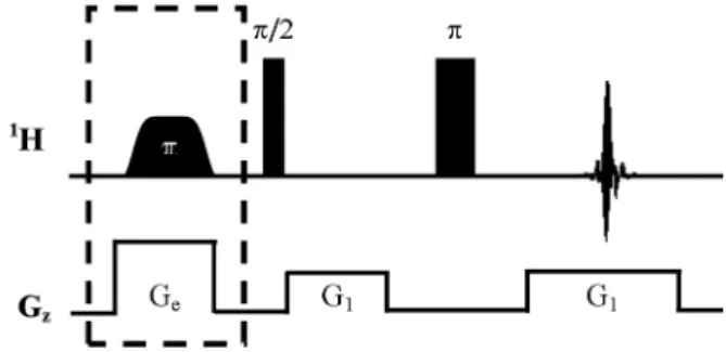
Spatially selective excitation is a fundamental step of UF-NMR experiments which needs to be carefully calibrated. Figure 1 describes the pulse sequence designed for this preliminary calibration. The first
step consists of calibrating the excitation pulses in order to ensure that their frequency width matches the frequency dispersion induced by the excitation gradients (Ge).
A sample with only one resonance frequency (here H2O in D2O) should be used for more efficient calibration. First, the dashed block (pulse calibration stage) is inactivated by setting the Ge strength to 0.0 G/cm and the selective pulse power level to 0.0 W. The rest of the sequence generates a spin echo which, after Fourier transform, yields the excitation profile of the sample (Figure 2a). Because of the phase dispersion induced by the gradients, a large first-order phase correction followed by a small zero order correction, are necessary to obtain a symmetric image.
The frequency dispersion induced by G1 corresponds to the width of the excitation profile (Figure 2b). In order to perform ul-trafast experiments, the gradient strength should be set to induce a frequency dispersion much higher than the chemical shift range, in order to ensure that all resonance frequencies are equally addressed at a given z position. Here, a 6.77 G/cm gradient is chosen, leading to a 54 kHz frequency dispersion, much higher than the usual 1H
spectral range. The next step consists of calibrating the adiabatic pulse used for spatial encoding. As discussed by Pelupessy,20 its bandwidth
should be slightly higher than the frequency dispersion induced by the gradients, to ensure that the whole sample is excited. The pulse calibration stage (Figure 1 - dashed block) is then activated, and the shaped pulse power level is decreased parametrically until complete inversion of the excitation profile is obtained (Figure 3S, supplemen-tary material). In our case the optimum shaped pulse power level was 0.32 W. This gradient calibration procedure need be performed only once, so the optimized parameters can be used for other experiments.
UF-COSY 2D implementation
With both shaped pulse and encoding gradient properly calibrated, we proceed to the implementation of a homonuclear bidimensional NMR experiment: Ultrafast COSY (UF-COSY). The pulse sequence used is shown in Figure 4S, supplementary material. For the afore-mentioned reasons, the constant-time spatial encoding proposed by Pelupessy20 was chosen to perform our experiments.
The UF-COSY pulse sequence starts with a nonselective π/2 pul-se, followed by constant-time spatial encoding in which two adiabatic pulses are applied simultaneously with a bipolar excitation gradient pair (Ge), leading to a spatially selective encoding of the spins. As the
phase has a quadratic dependence on z² after the first chirp pulse,20 it is necessary to apply a second pulse with an opposite gradient, to remove this effect and make the z-positions of the spins directly proportional to their resonance frequency. The mixing step is the same as for a conventional experiment, including coherence-selection gradients. A purge gradient (Gp) is used to shift the signal positions in the ultrafast dimension, in order to center them in the observation window. Finally, a bipolar acquisition gradient pair (Ga) is applied during 2.Ta, to refocus the dephasing induced by the spatial encoding
step, resulting in the formation of successive echoes according to the distinct precession frequency of the nuclei. This acquisition scheme is repeated N2 times leading to complete sampling of the (k, t2) space in
a single scan. The acquisition gradient amplitude Ga should be chosen
to ensure that the desired spectral width is observed in the spatially--encoded dimension. As a consequence, the maximum observable spectral width is limited by the maximum gradient amplitude availa-ble. While choosing Ga = 100% of the maximum gradient amplitude
would ensure the observation of the largest spectral range possible, we recommend instead to first set Ga = 70% to avoid reaching the
limits of the gradient hardware, principally to preserve its integrity but also because instabilities in the bipolar acquisition gradient train are observed for high Ga values. Ga can then be adjusted more finely depending on the spectral range to be detected.
Careful attention must be paid to shearing effects in the course of the acquisition process. Because of possible gradient offset, the positive acquisition gradient may not be the exact opposite of the negative gradient. This effect creates a linear shifting of the peak position during acquisition, leading to large resolution losses in the 2D spectrum. Therefore, fine tuning of the negative gradient amplitude must be performed to obtain optimum spectra.
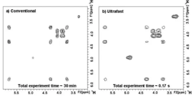
An example of UF-COSY 2D spectrum is given in Figure 3b for a Levamisol sample. The spectrum is recorded in 0.17 s, whereas 30 min are necessary to record its conventional counterpart (Figure 3a). The two spectra exhibit the same homonuclear correlations, thus proving the efficiency of the ultrafast approach.
UF-HSQC 2D implementation
The pulse sequence for implementation of the heteronuclear 2D HSQC experiment (UF-HSQC) is described in Figure 5S, supple-mentary material. The spatial encoding stage was performed on the
13C channel, therefore higher encoding gradients ±G
e were applied as
described in the experimental part in order to account for the larger
13C spectral range.
Figure 2. Image of the excitation profile obtained from the pulse sequence in Figure 1 (without the extra block), allowing for gradient strength calibra-tion. Without (a) and with (b) phase correccalibra-tion. The frequency dispersion Dω
induced by G2 is γ ·G2·L, where γ is the gyromagnetic ratio of detected nuclei and L the height of the detection coil. For both spectra, the acquisition time, number of data points and number of scans were 12.58 ms, 2984 and 1, respec-tively. For the processing parameters, the window function was the Gaussian multiplication with line broadening of -20.0 and Gaussian maximum position of 0.5 for both spectra, while the phase corrections of zero and first order were set to zero for spectrum 2a and to 11x106 and -23x106 for spectrum 2b
This UF-HSQC sequence has many steps in common with a conventional HSQC experiment. Initially, an INEPT block allows improving of the sensitivity of the 13C nuclei by polarization transfer
from the 1H nuclei. Subsequently, spatial encoding is performed on
the 13C channel to permit the position-dependent evolution of the 13C
nuclei, and in the middle of this period, a π pulse is applied on the
1H channel to refocus J
CH couplings. After a retro-INEPT block, the
signal is detected on the 1H channel. The echoes observed during
the first acquisition gradient correspond to the 13C spectrum, while
the 1H spectrum is obtained from the EPI dimension. Additionally,
π pulses are added on the 13C channel between acquisition gradients
to perform 13C decoupling.
As the ultrafast dimension window is limited by the strength of acquisition gradients, the spectral width observable in the 13C
di-mension is limited to a few tens of ppm.27 In order to overcome this
limitation, the recently proposed “gradient-folding” method27 to
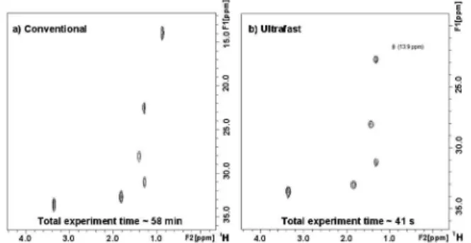
im-prove the spectral width of ultrafast 2D NMR experiments was used. The function of the gradients G1 and G2 is to enable the folding of the peaks that are outside the spectral window in the ultrafast dimension. The spectrum obtained after performing this UF-HSQC pulse sequence on a 1-bromohexane sample is shown in Figure 4b. Eight transients were accumulated for the sake of sensitivity and to per-form the conventional HSQC phase cycling for a more efficient coherence selection. However, the whole 2D spectrum is recorded in less than 1 minute, showing the same information as disclosed on the conventional spectrum (Figure 4a), but in a much shorter time-frame. The highlighted signal (13.9 ppm) in the ultrafast spectrum is folded in the ultrafast dimension by adjusting G1 (30 G/cm) and G2 (7.5 G/cm) gradients.
CONCLUSIONS
This paper describes a detailed protocol for implementing both homo- and heteronuclear multidimensional ultrafast experiments. In spite of its impressive performance, it should be noted that ultrafast NMR is characterized by several limitations and compromises which potentially affect its performance. In particular, a trade-off has to be made between resolution, sensitivity and spectral width, as descri-bed in recent papers.23,27,35 However, these limitations are now well
understood, and solutions have been proposed to overcome them. These solutions include, for example, the use of multi-echo excitation to limit sensitivity losses due to molecular diffusion24 or the use of
k-space folding strategies to increase the accessible spectral width.27,35
The sensitivity issues of ultrafast 2D NMR are also an important point worth discussing. The sensitivity of a single-scan experiment is of course lower than that of a conventional experiment where signal is accumulated for minutes or hours. This single-scan sensitivity is clearly highly dependent on the spectrometer and probe, but typically 100 mM samples are used in 400 MHz instruments equipped with conventional probes, while 10 mM samples are commonly used in 500 MHz instruments equipped with cryogenic probes.36 These values
seem quite high, but lower concentrations are easily reached by signal averaging, a “multi-scan single shot” approach whose potentialities have been recently demonstrated.37 Following these developments,
ultrafast NMR has been recently applied to a variety of situations, such as monitoring of fast organic reactions,28,38 the study of
biolo-gically relevant samples,30,38 coupling with hyphenated techniques39
and measurement of residual dipolar couplings in oriented media.40
We are currently applying these experiments to the study of dynamic processes occurring on a very short timescale that could not hitherto be followed by any other kind of 2D NMR experiment.
SUPPLEMENTARY MATERIAL
Free access in PDF format available on-line at http://quimicanova. sbq.org.br.
ACKNOWLEDGEMENTS
The authors are grateful to Prof. S. Akoka for discussions. P. Giraudeau acknowledges funding from the “Agence Nationale de la Recherche” (ANR Grant 2010-JCJC-0804-01). L. H. K. Queiroz Jr. and A. G. Ferreira acknowledge the Coordenação de Aperfeiçoamento de Pessoal de Nível Superior (CAPES), the Conselho Nacional de Desenvolvimento Científico e Tecnológico (CNPq) and the Fundação de Amparo à Pesquisa do Estado de São Paulo (FAPESP) for the financial support.
REFERENCES
1. Rabi, I.; Zacharias, J.; Millman, S.; Kusch, P.; Phys. Rev.1938, 53, 318. 2. Bloch, F.; Hansen, W.; Packard, M.; Phys. Rev.1946, 69, 127. 3. Purcell, E.; Torrey, H.; Pound, R.; Phys. Rev.1946, 69, 37.
4. Jeener, J.; International Ampere Summer School II, Basko Polje, Yugoslavia, 1971.
5. Aue, W. P.; Karhan, J.; Ernst, R. R.; J. Chem. Phys.1976, 64, 2229. 6. Lauterbur, P. C.; Nature1973, 242, 190.
7. Mansfield, P.; Maudsley, A. A.; J. Phys. C: Solid State Phys.1976, 9, L409.
8. Mandelshtam, V.; Taylor, H.; Shaka, A.; J. Magn. Reson.1998, 133, 304. 9. Kupče, Ē.; Freeman, R.; J. Magn. Reson.2003, 162, 300.
10. Brüschweiler, R.; Zhang, F.; J. Chem. Phys.2004, 120, 5253. 11. Schanda, P.; Brutscher, B.; J. Am. Chem. Soc.2005, 127, 8014. 12. Vitorge, B.; Bodenhausen, G.; Pelupessy, P.; J. Magn. Reson.2010, 207,
149.
13. Frydman, L.; Scherf, T.; Lupulescu, A.; Proc. Natl. Acad. Sci.2002, 99, 15858.
14. Gal, M.; Frydman, L. In Encyclopedia of NMR; Grant, D. M.; Harris, R. K., eds.; Wiley: New York, 2009, vol. 10.
15. Mishkovsky, M.; Frydman, L.; Annu. Rev. Phys. Chem.2009, 60, 429. 16. Tal, A.; Frydman, L.; Prog. Nuc. Magn. Res. Spec.2010, 57, 241. 17. Frydman, L.; Lupulescu, A.; Scherf, T.; J. Am. Chem. Soc.2003, 125,
9204.
18. Shrot, Y.; Frydman, L.; J. Magn. Reson.2003, 164, 351.
19. Shrot, Y.; Shapira, B.; Frydman, L.; J. Magn. Reson.2004, 171, 163. 20. Pelupessy, P.; J. Am. Chem. Soc.2003, 125, 12345.
21. Tal, A.; Shapira, B.; Frydman, L.; J. Magn. Reson.2005, 176, 107. 22. Shrot, Y.; Frydman, L.; J. Chem. Phys.2008, 128, 052209. 23. Giraudeau, P.; Akoka, S.; J. Magn. Reson.2008, 192, 151. 24. Giraudeau, P.; Akoka, S.; J. Magn. Reson.2008, 190, 339.
25. Pelupessy, P.; Duma, L.; Bodenhausen, G.; J. Magn. Reson.2008, 194, 169.
26. Giraudeau, P.; Akoka, S.; Magn. Reson. Chem.2011, 49, 307. 27. Giraudeau, P.; Akoka, S.; J. Magn. Reson.2010, 205, 171.
28. Queiroz Jr, L. H. K.; Giraudeau, P.; dos Santos, F. A.; de Oliveira, K. T.; Ferreira, A. G.; Magn. Reson. Chem.2012, 50, 496.
29. Giraudeau, P.; Lemeunier, P.; Coutand, M.; Doux, J.-M.; Gilbert, A.; Remaud, G. S.; Akoka, S.; J. Spectrosc. Dyn.2011, 1, 2.
30. Lee, M.-K.; Gal, M.; Frydman, L.; Varani, G.; Proc. Natl. Acad. Sci. 2010, 107, 9192.
31. Frydman, L.; Blazina, D.; Nat. Phys.2007, 3, 415.
32. Giraudeau, P.; Remaud, S.; Akoka, S.; Anal. Chem.2009, 81, 479. 33. Nagayama, K.; Kumar, A.; Wüthrich, K.; Ernst, R. R.; J. Magn. Reson.
1980, 40, 321.
34. Bodenhausen, G.; Ruben, D. J.; Chem. Phys. Lett.1980, 69, 185. 35. Shrot, Y.; Frydman, L.; J. Chem. Phys.2009, 131, 224516.
36. Giraudeau, P.; Massou, S.; Robin, Y.; Cahoreau, E.; Portais, J-C.; Akoka, S.; Anal. Chem.2011, 83, 3112.
37. Pathan, M.; Akoka, S.; Tea, I.; Charrier, B.; Giraudeau, P.; Analyst2011, 136, 3157.
38. Pardo, Z. D.; Olsen, G. L.; Fernández-Valle, M. E.; Frydman, L.; Martínez-Álvarez, R.; Herrera, A.; J. Am. Chem. Soc.2012, 134, 2706. 39. Queiroz Jr, L. H. K.; Queiroz, D. P. K.; Dhooghe, L.; Ferreira, A. G.;
Giraudeau, P.; Analyst2012, 137, 2357.
Supplementary Material
*e-mail: [email protected]
OPTIMIZATION AND PRACTICAL IMPLEMENTATION OF ULTRAFAST 2D NMR EXPERIMENTS
Luiz H. K. Queiroz Júnior*
Departamento de Química, Universidade Federal de São Carlos, Rod. Washington Luís, km 235, 13565-905 São Carlos – SP / Instituto de Química, Universidade Federal de Goiás, CP 131, 74001-970 Goiânia – GO, Brasil
Antonio G. Ferreira
Departamento de Química, Universidade Federal de São Carlos, Rod. Washington Luís, km 235, 13565-905 São Carlos – SP, Brasil Patrick Giraudeau
Université de Nantes, CNRS, Chimie et Interdisciplinarité: Synthèse, Analyse, Modélisation UMR 6230, B.P. 92208, 2 rue de la Houssinière, F-44322 Nantes Cedex 03, France
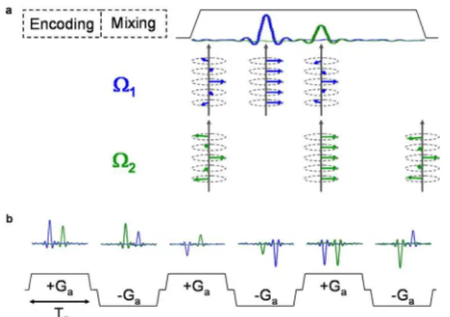
Figure 1S. (a) Graphical representation of continuous spatial encoding, in which a chirp pulse is applied concomitantly to a gradient pulse (Ge) along z axis. (b) The scheme proposed by Pelupessy20 comprises the application of a 90º hard pulse followed by two π chirp pulses applied together with a
bipolar pair of gradients
Figure 2S. (a) Representation of the ultrafast dimension acquisition by the application of a gradient pulse, in order to remove the dephasing created during the spatial encoding step. As result, the echo peaks are formed as the dephasing is being refocused. (b) Representation of the conventional dimension acquisition by the use of a bipolar pair of gradient pulses, which results in the monitoring of conventional parameters evolution as a series of sub-spectra are being collected
Figure 3S. Image of the excitation profile obtained from the pulse sequence in Figure 1 (with the extra block) and after phase correction, allowing for the chirp pulse power calibration before performing ultrafast experiments. The acquisition and processing parameters are the same mentioned for the Figure 2b, unless the chirp pulse power that was 0.32 W
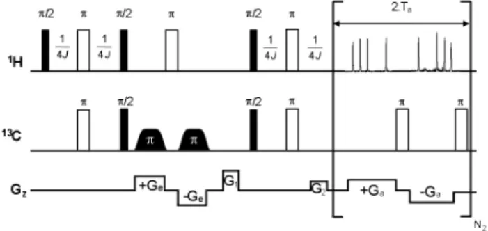
Figure 5S. Ultrafast HSQC pulse sequence based on the constant-time spatial encoding scheme proposed by Pelupessy.20 An asymmetric phase cycle (x,-x,x,x) was used within each single shot acquisition on the decoupling pulse to avoid the formation of decoupling artifacts. It was also used a real phase cycle (x,-x), requiring several scans, on the last 13C 90º pulse and the receiver. To perform this experiment, identical chirp pulses than those for UF-COSY were used, but applied in the presence of ± 20 G/cm encoding gradients to account for the larger 13C frequency range. The acquisition times for direct and indirect dimensions were 65.59 and 0.02 ms, respectively. Acquisition gradients were identical to those employed for UF-COSY. The INEPT delay was set to 1.72 ms. Eight scans were recorded for sensitivity and phase-cycling purposes
PULSE SEQUENCE FOR UF-COSY ;ufcosy
;avance-version
;$CLASS=HighRes ;$DIM=1D ;$TYPE= ;$SUBTYPE= ;$COMMENT=
#include <Avance.incl> #include <Grad.incl> #include <De.incl>
1 ze
100u UNBLKGRAD 2 d1 pl1:f1
p1 ph1 90º pulse
10u gron0
p11:sp1:f1 ph2 10u groff
10u gron1 spatial encoding block
p11:sp1:f1 ph4 10u groff 10u pl1:f1 10u
p23:gp23 coherence selection gradient 10u
p1 ph1 mixing period
10u
p26:gp26 coherence selection gradient
d25 gron25 purge gradient
10u groff 10u
ACQ_START(ph30,ph31) starting acquisition 1u DWELL_GEN:f1
3 d20 gron2 positive acquisition gradient
d6 groff gradient recovery delay d20 gron3 negative acquisition gradient d6 groff gradient recovery delay lo to 3 times l3 loop for acquisition rcyc=2
100u BLKGRAD
30m mc #0 to 2 F1QF(ip10, id0) exit
ph1=0 ph2=0 ph4=2 ph30=0 ph31=0
PULSE SEQUENCE FOR UF-HSQC ;ufhsqc
;avance-version
;$CLASS=HighRes ;$DIM=2D ;$TYPE= ;$SUBTYPE= ;$COMMENT=
#include <Avance.incl> #include <Grad.incl> #include <De.incl>
“p2=p1*2” “p4=p3*2” “d4=1s/(cnst2*4)” “d6=d4-d15” “d10=p20” “d11=p21”
“p15=(td*dw)/(2*l3)-2*d17-p4” 1 ze
100u UNBLKGRAD 2 30m pl2:f2
d1 pl1:f1
p1 ph0 d4
(center (p2 ph1) (p4 ph4):f2 )
d4 INEPT block p1 ph2
(p3 ph3):f2 d11 10u gron0
p7:sp1:f2 ph1 10u groff
d10 10u
p2 ph1 spatial encoding block 10u
10u gron1 180º pulse p7:sp1:f2 ph1
10u groff
(p3 ph5):f2
(p1 ph1) retro-INEPT block d4
(center (p2 ph1) (p4 ph4):f2 ) d6
d15 gron5 coherence selection and folding gradient 10u groff
10u
d15 gron7 purge gradient
10u groff
ACQ_START(ph30,ph31) starting acquisition 1u DWELL_GEN:f1
3 p15:gp15 positive acquisition gradient
d17 recovery delay
(p4 ph6):f2 decoupling pulse
d17 recovery delay
p15:gp16 negative acquisition gradient
d17 recovery delay
(p4 ph6):f2 decoupling pulse
d17 ipp6 recovery delay / phase (ph6) increment
lo to 3 times l3 loop for acquisition rcyc=2
100u BLKGRAD
30m mc #0 to 2 F1QF(id2) exit
ph0=0 ph1=0 ph2=1 ph3=0 ph4=0 ph5=0 2
ph6=0 2 0 0 asymmetric phase cycle on the decoupling pulse to avoid the formation of decoupling artifacts