The “running in the rain” problem revisited:
an analytical and numerical approach
(O problema “correndo na chuva” revisitado: uma abordagem anal´ıtica e num´erica)
T. Kroetz
1Departamento de F´ısica, Instituto Tecnol´ogico de Aeron´autica, Centro T´ecnico Aeroespacial, S˜ao Jos´e dos Campos, SP, Brazil
Recebido em 31/3/2009; Revisado em 23/6/2009; Aceito em 7/7/2009; Publicado em 18/2/2010
The dependence between the speed of an object that travels a given distance through the rain and the volume of water dumped on it by the raindrops is examined in this work. Considering a model based on the average distance between the raindrops, it is possible to obtain an analytical equation that expresses this dependence in terms of physical rain parameters. In order to verify our results a more realistic and sophisticated model considering the random nature of the raindrops distribution in the space was built.
Keywords: running in the rain, raindrops distribution.
A dependˆencia entre a velocidade com a qual um objeto percorre uma determinada distˆancia na chuva e o volume de ´agua despejado nele pelas gotas ´e examinada neste trabalho. Considerando um modelo baseado na distˆancia m´edia entre as gotas ´e poss´ıvel obter uma equa¸c˜ao anal´ıtica que expressa esta dependˆencia em termos dos parˆametros f´ısicos da chuva. A fim de verificar nossos resultados constru´ımos um modelo mais realista e sofisticado que considera a natureza randˆomica da distribui¸c˜ao de gotas de chuva no espa¸co.
Palavras-chave: correndo na chuva, distribui¸c˜ao de gotas de chuva.
1. Introduction
The theoretical physics methodology is based on the construction of models that represent the real system which is intended to be studied. The models preserve the essential features and discard the less important details to the systems description through the suitable choices of assumptions and simplifications. Analyzing a model is possible to obtain comparable results with experimental measures of the real system and so the model can be considered plausible or refuted. In the present work this methodology is didactically exempli-fied through a curious question: What is the best speed to cross a certain distance under rain (without an um-brella) in order to arrive as dry as possible?
This problem was investigated in previous works. In [1] was obtained an analytical expression, derived from a flux argument, which gives the number of raindrops hitting one inclined plane crossing the rain in terms of its horizontal velocity. Another equivalent expression is developed in [2] for a rectangular parallelepiped run-ning in the rain considering the apparent inclined di-rection of the raindrops trajectory due to the speed of the object. The last work mentioned applied the idea of
average distances of the raindrops. This concept is also used in our approach but in a different way. Both works do not consider the lateral velocity of drops. In [3] the author investigates the problem with a model consider-ing a “volume of rain per unit volume of air”includconsider-ing the lateral incidence of drops. The conclusions of these works are the same: if the object travels faster it will arrive drier, excepting when the horizontal velocity of the rain is in the same direction as the motion of the object. They also agreed that there is a limit of rain-drops collected by the object when its velocity goes to infinity, indicating that there are no great advantages on running at very fast speeds instead of at a standard speed. However, they are unclear on how the parame-ters of the models are related to the real rain ones (like precipitation rate and volume of the drops), so that the comparison of the results with any experiment becomes very difficult to be done (or maybe impossible).
A new model was built in this work, describing the rain as a three-dimensional lattice, moving towards each direction at velocity components of the raindrops. An analytical expression in terms of physical rain para-meters is obtained through the model. The expression gives water volume dumped on one object as function
1E-mail: [email protected].
of velocity at which it travels a certain distance un-der the rain. This expression is completely comparable with experimental results because all the terms pre-sented in the final theoretical relation are measurable. In addition to it, a more complex model that makes use of a computational algorithm was created in order to confront the results extracted from the analytical ex-pression. As the work only requires basic principles of physics and math and includes a detailed mathematic development of the final relation, the paper becomes interesting to the physics education. It provides an elu-cidative example of the theoretical physics methodol-ogy to the undergraduate students in the first years of physics graduation course.
2.
The Lattice Rain Model (LRM)
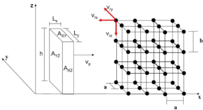
In order to obtain an expression that gives the wa-ter volume dumped on one object at the end of its travel under the rain, we constructed a model prob-lem called “Lattice Rain Model” (LRM). In this model, the rain consists of a three-dimensional lattice with tetragonal unit cell where each lattice element corre-sponds to one raindrop. There are two characteristic cell edges: one horizontal a and one vertical b. Each lattice element moves in (x, y, z) coordinates at the ve-locity components of the rain (vrx, vry, vrz) respectively.
This construction was based in the assumption that, for a homogenous rain, the distance between one rain-drop and its neighbor along one coordinate axis is very similar to the average distance between each drop and its respective neighbors in this same axis. Consider-ing an isotropic rain alongxand y directions, the cell edges must be equal in these directions. The velocities (vrx, vry, vrz) are constant. The vertical direction
ve-locityvrzcan be considered constant because drops fall
only a few meters before reaching the terminal veloc-ity [4].
In order to represent a person running in the rain, a box with horizontal, frontal and lateral areas: Axy,Ayz
and Axz respectively is taken into consideration. The
object moves along thex-direction with velocityvp for
a distanceD. A representation of the model problem is shown in Fig. 1. Only a piece of the lattice is rep-resented in the scheme, but is considered that it would fill all the space.
Defining t′ = b/|v
rz| as the time between two
consecutive horizontal planes of the lattice reach the ground, we expressbas
b=t′|vrz|, (1)
where t′ has an unknown value for while. In order to
relateaandbwith the real rain parameters, a measure of rain intensity commonly called “precipitation rate”P
is introduced. This parameter is defined in terms of the volume of water V dumped on an arbitrary horizontal areaAhduring the time tas
Figure 1 - Representation of the LRM. The distance between two consecutive vertical (horizontal) rain planes isa(b).
P = V
Aht
, (2)
and, in general, it is given in units of mm/h. In our calculations, the MKS system is used, i.e., P will be given in units of m/s. If we use Axy as the horizontal
area andt′ as the time in Eq. (2), it is possible to
ob-tain the water volume conob-tained in just one horizontal plane (see the definition oft′ above) of the lattice with
the same area of the top of the body.
Vxy=P Axyt′. (3)
On the other hand, the number of drops in one hor-izontal plane of rain lattice with sides Lx and Ly is
given, as we can see in Fig. 2 (a), by
Nxy=
Lx
a Ly
a =
Axy
a2 , (4)
Therefore, ifVdis the volume of each drop, the volume
Vxy can also be represented by
Vxy=Vd
Axy
a2 . (5)
The Eqs. (3) and (5) were obtained independently. While the definition ofP was used to get the first, the lattice parameteraassociated with the rain parameter
Vd were used to get the second one. Equaling the right
sides of these equations, the lengthacan be expressed by
a=
r
Vd
t′P. (6)
The number of drops in one frontal plane of rain lattice with sides Ly and h is given, as we can see in
Fig. 2 (b), by
Nyz =
Ly
a h
b = Ayz
ab . (7)
Similarly, the number of drops in one lateral plane of the rain lattice with sidesLx andhis given by
Nxz =
Lx
a h b =
Axz
Using Eqs. (1) and (6) in Eqs. (7) and (8) is possible to obtain the expressions
Nyz =
Ayz
|vrz| r
P t′V d
, (9)
and
Nxz =
Axz
|vrz| r
P t′V d
. (10)
MultiplyingNyz andNxz respectively by the
num-ber of frontal and lateral rain planes crossed by the body in its movement, it is possible to obtain the num-ber of raindrops hitting it on each side at the end of the travel. The water volume dumped on the body on
Ayz (Axz) is calledVF (VL) and it is given by the drop
volumeVdmultiplied byNyz (Nxz) and the number of
frontal (lateral) planes crossed by the body during the travel
VF =Vd
|vp−vrx|t
a Nyz, (11)
VL=Vd
|vry|t
a Nxz, (12)
where the number of planes crossed in one direction is written as the travel timetmultiplied by relative veloc-ity between the body and the rain along the considered direction and divided by the distance between to con-secutive planes. The absolute value of relative velocities were used because the number of raindrops hitting the body can not be negative.
Replacinga,NyzandNxz in the Eqs. (11) and (12)
by the expressions (6), (9) and (10) respectively, the frontal and lateral volume will be given by
VF =P
|vp−vrx|t
|vrz|
Ayz, (13)
Figure 2 - Drops contained in (a) one horizontal plane of lat-tice of sidesLx andLy and (b) one frontal plane of lattice
of sidesLyandh.
VL=P
|vry|t
|vrz|
Axz. (14)
It is interesting to observe that the arbitrary parameter
t′ was vanished when the number of drops in one plane
was multiplied by the number of planes crossed by the body, although we define the lattice characteristic cell edgeb in terms of it. The parametert′ was important
on the mathematical development, but the final result does not depend on any specific choice oft′ value. The
volume of water dumped on the top of the bodyVT will
be given by the expression (2) replacingAhbyAxy
VT =P tAxy. (15)
The total water volume on the body when it finishes its travel will be the sum of expressions (13), (14) and (15).
Vtotal=P t ·
Axy+
|vp−vrx|
|vrz|
Ayz+
|vry|
|vrz|
Axz ¸
, (16)
wheretis the travel time. The travel time will be given by the expressionD/vp when the distanceD is
prede-termined. So the Eq. (16) assumes the form
Vtotal=P D "
Axy
vp
+|1−
vrx
vp|
|vrz|
Ayz+
|vry|
|vrz|vp
Axz #
.
(17) The limits of Eq. (17) are
lim
vp→0
Vtotal=∞, (18)
lim
vp→∞
Vtotal=P D
Ayz
|vrz|
. (19)
The above limits indicate thatVtotaldecreases from the
infinity (forvp= 0) to a non-zero value whenvp → ∞.
For a negative value of vrx (the x-velocity of the rain
against the motion of the body), the numerator of the middle term in the brackets of Eq. (17) is always greater than unity (sincevp is positive by definition) and tends
to one as vp → ∞. It indicates that there is no
mini-mum in the functionVtotal(vp) and it decreases
asymp-totically to the limit value of Eq. (19). Therefore, the best speed to run for a distance D through the rain which presents horizontal velocity against the runner’s motion would be the fastest one that might be possible to reach, in order toVtotal becomes as close as possible
toP DAyz
|vrz|.
However, ifvrxis positive (thex-velocity of the rain
in the same direction as the motion of the object), then there is an optimal velocity vp =vrx that cancels the
value ofvpthe total water volume dumped on the body
at the end of the travel is given by
Vtotal(vp=vrx) =P D ·A
xy
vrx
+ |vry|
|vrz|vrx
Axz ¸
. (20)
It is possible to wonder if it would be better to run as rapidly as possible or at the speedvp=vrx in order to
arrive drier, in case of a positive value forvrx. In other
words: is it better to cancel the middle term or the first and third terms in Eq. (17)? The first option will be better when the right side of Eq. (20) has a lower value than the right side of Eq. (19). This will occur when
vrx> v∗rx=
|vrz|
Ayz ·
Axy+
|vry|
|vrz|
Axz ¸
, (21)
where v∗
rx is the value of x-velocity of the rain which
obeys the relation Vtotal(vp = v∗rx) = limvp→∞Vtotal.
If vrx < vrx∗ and vp =vrx, then the water volume on
the area Ayz remains zero, but the body spends too
much time crossing the distanceD and the water vol-ume dumped on its top and lateral areas makes the option of running at a velocity vp = vrx not the best
one.
3.
The Random Rain Model (RRM)
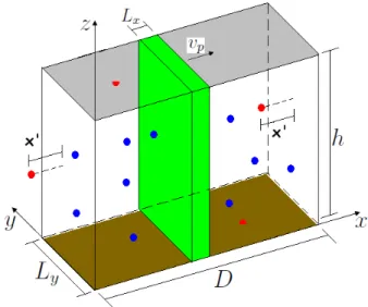
Could the results obtained with the LRM remain valid for a real rain? A conclusive answer to this question can only be given through a comparison between ex-perimental results and the theoretical ones, extracted from the Eq. (17), but this is not the scope of this work. However, a more sophisticated and totally independent model could be elaborated in order to confront results. It considers the main differences between the lattice model and the real rain: the random position of drops formation and the individual movement of each drop. This model is called “Random Rain Model”(RRM). The only way to extract results from it is making use of a computational algorithm2.
The algorithm considers a rain confined in a rectan-gular parallelepiped of sides D (distance to be crossed by the body), Ly (width of the object) and h(height
of the object). Each drop is formed on the top of the parallelepiped, after the time intervaldt since the pre-vious drop was created. The initial horizontal posi-tion of the drops is chosen randomly, i.e., (x0, y0, z0) =
(rand×D, rand ×Ly, h), where rand is a random
number into the interval (0,1). The i-th drop moves according the cinematic equations: (x(i), y(i), z(i)) =
(x(i)0 +vrxt(i), y0+vryt(i), z (i)
0 +vrzt(i)), where t(i) is
the time passed since when the i-th drop was formed. The velocities (vrx, vry, vrz) are the same for all drops.
The boundary conditions of the space is cyclic on laterals. This means that when a drop crosses one side of the parallelepiped, leaving the space, it reappears on
the opposite side preserving the other two coordinates. Every time a drop reaches the floor it is eliminated by the algorithm and another drop is created on the top of space at a new random initial position (x0, y0). So,
the number of drops into the parallelepiped is always the same. The parallelepiped space represents a piece of a rain as a whole. The justification of the RRM cyclic lateral boundary condition is due to the assump-tion that the piece of rain considered repeats almost identically along x-direction and y-direction for a ho-mogeneous real rain. In other words, the RRM only permits only new drop information entering into the space from the top area.
While the drops are moving in the space as de-scribed above, a rectangular object of dimension Lx,
Ly andhmoves inx-direction through the distance D
at velocityvp. The algorithm counts every drop hitting
the lateral, frontal and back area of the body during its travel. Because the space has the same height of the object, a drop hitting the top area of the body is counted when the initial horizontal position of the drop is contained on the top area of the object at the time of drop creation. At the end of the travel alongD, the water volume dumped on the body is obtained multi-plying the total number of hitting drops counted by the volume of the dropVd chosen. A representation of the
RRM is shown in Fig. 3.
Figure 3 - Representation of the RRM. The red drops are crossing the boundaries of the space. When one drop reaches the floor, another one is created on the top. When one passes a distancex′over one side of the space, it reappears
at a distancex′ of the opposite side. The same occurs for
the y-direction (not shown in figure). The sizes of drops, body and the space are not in scale.
The drop formation time intervaldtand the volume of the drop Vd are directly related to the precipitation
rate P. For the RRM, it is known that if the time of rain exposure isdt, then the water volume dumped is
the volume of just one drop Vd. So, for the RRM, the
precipitation rate will be given by
P= Vd
DLydt
, (22)
where DLy is the area of the floor which receives the
rain incidence. In order to relate the numerical para-meter dt with the real rain parameters P and Vd, dt
was placed on the left side of Eq. (22)
dt= Vd
P DLy
. (23)
4.
Results
The water volume dumped on the object for several val-ues of vp were obtained from LRM and RRM and the
two functions were plotted in the same graph. The same value of parameters in both models were used in order to compare the results. The precipitation rate will be taken asP = 4 mm/h = 1.11×10⁻⁶ m/s (a moderate
rain). The body dimensions assume values close to hu-man body dimensions: Lx = 0.2m,Ly = 0.4 m andh
= 1.8 m. Consequently, the areas in Eq. (17) will be
Axy=Lx×Ly = 0.08 m2,Ayz =Ly×h= 0.72 m2and
Axz =Lx×h= 0.36 m2. The travel distance and the
lateral rain velocity will be chosen as D = 100 m and
vry= 3 m/s. The terminal velocityvrzdepends on the
size of the drops. For a drop with radiusr= 1.375 mm (Vd = 1.089×10⁻⁸ m3) the terminal velocity is about
vrz = -7.75 m/s [4]. The time interval of drop
forma-tion in the RRM must be dt = 2.45×10⁻⁴ when the
above values for Vd, P, D and Ly are inserted in the
Eq. (23).
When thevrx is negative (positive), the drops hits
the frontal (back) area of the body. Moreover, positive and negative values ofvrxmust be analyzed separately
in order to explore this two different situations.
4.1. The x-velocity of the rain against the
mo-tion of the body
If we choose the valuevrx = -3 m/s forx-direction
ve-locity, the dependence between Vtotal and vp, for each
model, is shown on Fig. 4. The absence of minimum in the graph allows to conclude that the object should travel the distanceD as fast as possible in order to ar-rive drier. However, as the relation between Vtotal and
vp is not linear, the gain running at very fast speed
could not be very significant in comparison to running at moderate speed. For example: travelling at 5 m/s (a normal run) the object arrives 68% less wet than if it travels at 1 m/s (a slow walk). But if it runs at 10 m/s (close to world record speed) it will arrive just 74% less wet than at 1 m/s. The gain difference is only 6% while the run is 100% faster than 5 m/s.
Figure 4 - Variation of the water volume dumped on the body as a function of its velocityvp, forvrx= -3 m/s. The
red line corresponds the LRM results, and the black one the RRM results. The square indicates a region which was zoomed and it is shown in the same figure.
It is possible to observe that the results obtained from LRM and RRM show great similarities. As the RRM is a model based on random variables, conse-quently its results will be different each time we run the algorithm. However, the difference will just be a statistical fluctuation, and the general behavior will be always the same. The LRM is a model based on the average distances of the raindrops horizontally and ver-tically. Since LRM ignores the statistical fluctuation on the distances, the red curve in Fig. 4 is smooth and just represents the general behavior of the RRM results.
4.2. The x-velocity of the rain on the same
di-rection of motion of the body
In section 2., it was predicted that there is an optimal velocity that cancels the drops incidence on the frontal (or back) areaAxz for a positive vrx. But, when the
value ofvrx is small, it could not worth to run at this
velocity because the body would be exposed to the rain for an extremely long time. The Eq. (21) gives the lower limit of vrx which makes Vtotal a minimum for
vp=vrx. Substituting the values ofvry, vrz,Ayz, Axy
andAxz used in simulations in Eq. (21), we find that
this limit must bev∗
rx= 2.361 m/s.
In order to test the expression (21), we plot two de-pendencies between V and vp with positive vrx. The
plot shown on Fig. 5 is for vrx = 2 m/s (a lower
value than v∗
rx). The plot shown in Fig. 6 is for
vrx = 3 m/s (a higher value thanv∗rx). The similarity
between LRM and RRM is verified again. In adition to it, we can check that whenvrx> vrx∗ , the object arrives
drier when running at the speed vp =vrx. In case of
vrx< vrx∗ , the idealvpis the fastest as possible (as seen
Figure 5 - Variation of the water volume dumped on the body as a function of its velocityvpwithvrx= 2 m/s, for
LRM (red) and RRM (black). The square indicates a zoom region close to vp = vrx. The velocity vp = 2 m/s is a
discontinuity of the function but not a minimum.
Figure 6 - Variation of the water volume dumped on the body as a function of its velocityvpwithvrx= 3 m/s, for
LRM (red) and RRM (black). The square indicates a zoom region close to vp = vrx. The velocity vp = 3 m/s is a
discontinuity and a minimum of the function.
5.
Conclusions
Two models have been proposed that enable the study the “running in the rain”problem. The LRM considers a rain with drops in sites of a three-dimensional lat-tice. An analytical expression which gives the relation between the speed of a running body under the rain and the water volume on it at the end of its travel was obtained through this model. The second model is the RRM, a numerical model which considers each drop in-dividually (and not on equidistant planes, as considered by LRM) and being formed on random initial positions. Although the RRM reproduces more authentically the main features of the real rain, the results obtained by RRM and LRM are almost identical. The difference resides in small statistical fluctuations on RRM results which will be distinct each time we run the algorithm
(since it uses random variables). The details included in the RRM do not contribute significantly to a refined re-sult. It also can not provide an analytic relation as the LRM. So, the main role of RRM was to give credibility to Eq. (17). The main goal of this work is to obtain the-oretical results that can be comparable to experimental results, since all parameters present in Eq. (17) can be known experimentally. It is also a simple and didactic example on how the theoretical physics methodology works.
The results from this work indicate that when the rain falls perpendicularly to the top area of the body, or hitting it on its frontal area, the best speed to cross the rain is as fast as possible. Although running being better than walking, the advantages of running faster than a conventional speed run could not worth the ad-ditional effort, as it was already observed in [2]. In case of the rain hitting the body on its back area, it could be better to run at the velocity component of the rain parallel to the motion of the body. Considering the Eq. (21) it is possible to decide if running at this spe-cific speed is the best option or not. This calculation is a bit unpractical on the daily life as a requisite to take a decision. There are alternative solutions which are more convenient to be applied. For exemple: the per-son who needs to run in the rain could just observe the inclination of drops trajectory in relation of his back area and intuitively assess if the lower limit of Eq. (21) is respected or not. Even when vrz < v∗rz, the water
volume decreases drastically forvp=vrzand passes to
decrease slowly for vp > vrz, as we can see in Fig. 5.
Consequently, there is no great advantages on running at a speed much faster thanvp=vrz.
The theoretical results obtained from the models are no longer applicable in everyday life when the distance
D is extremely extensive. There is a limit on how wet a person could get, because after that the body is con-sidered soaked and even if more drops hit it, the body can not get wetter. When the distance D is very long, this limit can be achieved. So, a person who needs to cross a long distance in the rain would walk quietly for not getting tired (unless he/she feels cold).
6.
Acknowledgments
The author would like to thank Alexandre M. Zabot for the encouragement, revision and helpful discussions.
Referˆ
encias
[1] S.A. Stern, American Journal of Physics 51, 815 (1983).
[2] A. De Angelis, European Journal of Physics 8, 201 (1987).
[3] H. Bailey, The College Mathematics Journal 33, 88 (2002).