Mitigation of Magnetic Field under Egyptian 500kV
Overhead Transmission Line
Adel Z. El Dein
Abstract—The paper presents an efficient way to mitigate the magnetic field resulting from the three-phase 500kV single circuit high voltage transmission line existing in Egypt, by using a passive loop conductor. The aim of this paper is to reduce the amount of land required as rights-of-way (ROW). The paper used an accurate method for the evaluation of 50Hz magnetic field produced by overhead transmission lines. This method is based on the matrix formalism of multiconductor transmission lines (MTL). This method obtained a correct evaluation of all the currents flowing in the MTL structure, including the currents in the subconductors of each phase bundle, the currents in the ground wires, the currents in the mitigation loop, and also the earth return currents. Furthermore, the analysis also incorporates the effect of the conductors sag between towers, and the effect of sag variation with the temperature on the calculated magnetic field. Good results have been obtained and passive loop conductor design parameters have been recommended for this system at ambient temperature (35oC).
Index Terms—Magnetic Field, Mitigation loop, Right-of-way, Transmission lines
I. INTRODUCTION
HE rabid increase in HV transmission lines and irregular population areas near the manmade sources of electrical and magnetic fields, in Egypt, needs a suggestion of methods to minimize or eliminate the effect of magnetic and electrical fields on human begins in Egyptian environmental areas especially in irregular areas. Public concern about magnetic field effects on human safety has triggered a wealth of research efforts focused on the evaluation of magnetic fields produced by power lines [1], [2]. Studies include the design of new compact transmission line configurations; the inclusion of auxiliary single or double lops for magnetic field mitigation in already existing power lines; the consideration of series-capacitor compensation schemes for enhancing magnetic field mitigation; the reconfiguration of lines to high phase operation, etc [3]-[5]. However, many of the studies presented that deal with power lines make use of certain simplifying assumptions that, inevitably, give rise to inaccurate results in the computed magnetic fields. Ordinary simplifications include neglecting the earth currents, neglecting the ground wires, replacing bundle phase conductors with equivalent single conductors, and replacing actual sagged conductors with average height Horizontal conductors. These assumptions result in a model where magnetic fields are distorted from those produced in reality [6], [7]. In this paper, a matrix-based MTL model [8], where the effects of earth currents, ground wire currents and mitigation loop current are taken into account, is used; moreover, actual bundle conductors and conductors’ sag at various temperatures are taken into consideration. The
results from this method without mitigation loop are compared with those produced from the common practice method [6], [7] for Magnetic field calculation where the power transmission lines are straight horizontal wires of infinite length, parallel to a flat ground and parallel with each other. Then the optimal parameters of the mitigation loop design for Egyptian 500kV overhead transmission line are obtained.
II. COMPUTATION OF SYSTEM CURRENTS
The MTL technique is used in this paper for the simple purpose of deriving the relationship among the line currents of an overhead power line. This method is explained in [8], this paper reviews and extends this method for Egyptian 500kV overhead transmission line, with an other formula for the conductors’ sag, taken into account the effect of temperature on the sag configuration [9]. The first step required to conduct a correct analysis consists in determination of all system currents based on prescribed phase-conductor currents Ip:
I
1;
I
2;
I
3
I
p
(1)Consider the frequency-domain transmission line matrix equations for non-uniform MTLs (allowing the inclusion of the sag effect)
I
z
Z
dz
dV
/
`(
,
)
(2a)V
z
Y
dz
dI
/
`(
,
)
(2b)Where Z` and Y`, denote the per-unit-length series-impedance and shunt-admittance matrices, respectively ,V and I are complex column matrices collecting the phasors associated with all of the voltages and currents of the line conductors, respectively.
L G p p p
n L
n G
n c
n b
n a
V
V
V
V
V
V
1 1 1 1 1
and
L G p p p
n L
n G
n c
n b
n a
I
I
I
I
I
I
1 1 1 1 1
(3)
In (3), subscripts a, b, and c refer to the partition of phase bundles into three sub-conductor sets. Subscript G refers to ground wires and L subscript refers to the mitigation loop. In (3) np, nG, and nL denote, the number of phase bundles, the
number of ground wires, and the number of conductors in the mitigation loop, respectively, for the Egyptian 500kV overhead transmission line it is seen that: np = 3, nG =2, and
nL = 2 as it is proposed in this paper. Since the separation of
T
quasistationary regimes (50Hz), where wave-propagation phenomena are negligible, all system currents are assumed to be Z independent. This means the transversal displacement currents among conductors are negligible or, in other words, (2b) equates to zero and only Z` values are needed to calculate. Since the standard procedure for computing Z` in (2a) has been established elsewhere [10]-[12], details will not be revealed here and thus only a brief summary is presented.
skin
E
Z
Z
L
j
Z
`
(4)The external-inductance matrix is a frequency-independent real symmetric matrix whose entries are:
)
/
2
ln(
)
2
/
(
o k kkk
y
r
L
(5a)2 2
2 2
)
(
)
(
)
(
)
(
ln
4
i k i kk i k
i o kk
x
x
y
y
x
x
y
y
L
(5b)Where
r
k denotes conductor radius, andy
k andx
k denote the vertical and horizontal coordinates of conductor k. Matrix ZE , the earth impedance correction, is a frequencydependent complex matrix whose entries can be determine using Carson’s theory or, alternatively, the Dubanton complex ground plane approach [10]-[12]. The entries of ZE
are defined as:
Z
E kk
(
j
o/
2
)
ln
1
/
y
k
(6a)
2 2 2 2
) (
) (
) (
) 2 (
ln
4 i k i k
k i k
i o ik
E
x x y
y
x x y
y j
Z
(6b)where
, the complex depth, is given by2 / 1
)
/
(
j
o
with ρ denoting the earth resistivity.Matrix Zskin is a frequency-dependent complex diagonal
matrix whose entries can be determined by using the skin-effect theory results for cylindrical conductors [7].
For low-frequency situations, it will be:
Z
skin
kk
(
R
dc)
k
j
(
o/
8
)
(7)Where
(
R
dc)
kdenotes the per-unit-length dc resistance of conductor k. Due to the line conductors' sag between towers; yk will be a function on the distance z between the twotowers, also the entries for L and ZE, defined in (5) and (6),
vary along the longitudinal coordinate z. The exact shape of a conductor suspended between two towers of equal height can be described by such parameters; as the distance between the points of suspension span, d, the sag of the conductor, S, the height of the lowest point above the ground, h, and the height of the highest point above the ground, hm. These parameters can be used in different combinations [13], [14]. Fig. (1) depicts the basic catenary geometry for a single-conductor line, this geometry is described by:
))
2
/(
(
sinh
2
k 2 kk
k
h
z
y
(8)Where
k is the solution of the transcendental equation:)
(
sinh
]
/
)
[(
2
hm
k
h
kd
ku
k
2u
k , for conductor k; with)
4
/(
kk k
d
u
. The parameter
kis also associated with the mechanical parameters of the line:
k
(
T
h)
k/
w
kwhere
(
T
h)
k is the conductor tension at mid-span andw
kis weight per unit length of the conductor k.Fig. 1. Linear dimensions which determine parameters of the catenary.
Consider a mitigation loop of length l, is present, where l is a multiple of the span length d. The line section under analysis has its near end at -1/2 and its far end at l/2.
The integration of (2a) from z = -l/2 to z = l/2 gives:
/22 /
)
`(
l l far
near
V
I
Z
z
dz
V
(9a)Equation (9a) can be written explicitly, in partitioned form, as:
L G c b a
LL LG Lc Lb La
GL GG Gc Gb Ga
cL cG cc cb ca
bL bG bc bb ba
aL aG ac ab aa
L G c b a
I I I I I
Z Z Z Z Z
Z Z Z Z Z
Z Z Z Z Z
Z Z Z Z Z
Z Z Z Z Z
V V V V V
(9b)
The computation of the bus impedance Z in equation (9) is performed using the following formula:
/22 /
)
`(
l l
dz
z
Z
Z
(10)Where values for Z` are evaluated from equations (4-7) considering the conductors' heights given by (8). The two-conductor mitigation loop is closed and may include or not a series capacitor of impedance Zc [5]. In any case, the
submatrix IL in (3) has the form:
TL L L
L
I
I
S
I
1;
2
I
(11)where;
S
1
1
By using the boundary conditions at both the near and far end of the line section, the voltage drop in the mitigation loop will be:
Original span
d2 d
d1
K=-1 K=0 P1 P2 K=1
X
h s Y
hm
L c L L far L L near L L L L L Z V V V V V V V V V I 1 1 2 1 2 1 2 1
which can be written as:
L c L
L
L
V
V
Z
V
S
1
2
I
(12)Where
I
Lis the loop current, andZ
c
jX
s
1
/(
j
C
s)
isthe impedance of the series capacitor included in the loop. Using (12), the fifth equation contained in (9b) allows for the evaluation of the currents flowing in the mitigation loop.
G K LG T c K Lc T b K Lb T a K La T L L L I SZ YS I SZ YS I SZ YS I SZ YS I LG Lc Lb La I ; I (13)
Where ;
Y
1
/(
Z
c
SZ
LLS
T)
Taking into account that the conductors belonging to given phase bundle are bonded to each other, and that ground wires are bonded to earth (tower resistances neglected), that result in:
c b
a
V
V
V
and
V
G
0
By using
V
G
0
in the fourth equation contained in (9b)and using equation (13), the ground wire will be:
c K Lc GL Gc G b K Lb GL Gb G a K La GL Ga G
G Y Z Z K I Y Z Z K I Y Z Z K I
I Gc Gb Ga ( ) ( ) ( ) (14)
Where;
Y
G
(
Z
GLK
LG
Z
GG)
1Next, by using (13) and (14), IL and IG can be eliminated in
(9b), yielding a reduced-order matrix problem:
c b a cc cb ca bc bb ba ac ab aa c b a I I I Z Z Z Z Z Z Z Z Z V V V ˆ ˆ ˆ ˆ ˆ ˆ ˆ ˆ ˆ (15)
where ;
Z
ˆ
aa
Z
aa
Z
aGK
Ga
Z
aL(
K
La
K
LGK
Ga)
)
(
ˆ
Gb LG Lb aL Gb aG abab
Z
Z
K
Z
K
K
K
Z
)
(
ˆ
Gc LG Lc aL Gc aG acac
Z
Z
K
Z
K
K
K
Z
)
(
ˆ
Ga LG La bL Ga bG baba
Z
Z
K
Z
K
K
K
Z
)
(
ˆ
Gb LG Lb bL Gb bG bbbb
Z
Z
K
Z
K
K
K
Z
)
(
ˆ
Gc LG Lc bL Gc bG bcbc
Z
Z
K
Z
K
K
K
Z
)
(
ˆ
Ga LG La cL Ga cG caca
Z
Z
K
Z
K
K
K
Z
)
(
ˆ
Gb LG Lb cL Gb cG cbcb
Z
Z
K
Z
K
K
K
Z
)
(
ˆ
Gc LG Lc cL Gc cG cccc
Z
Z
K
Z
K
K
K
Z
The relationship between Ia , Ib and Ic is obtained from (15)
by making
V
a
V
b
V
c and by usingp c b
a
I
I
I
I
. Then the following relations are obtainedp bc
ac ac
a
KK
KK
K
I
I
(
1
)
1 (16a)p bc
ac bc
b
KK
KK
K
I
I
(
1
)
1 (16b)p bc
ac
c
KK
K
I
I
(
1
)
1 (16c)Where ;
KK
ac
KK
abKK
bc
KK
ac)
ˆ
ˆ
(
bb aba
ab
Y
Z
Z
K
;K
ac
Y
a(
Z
ˆ
bc
Z
ˆ
ac)
1)
ˆ
ˆ
(
aa baa
Z
Z
Y
;K
bc
(
K
bc1)
1K
cb1 bb ab ba cb ab cabc
Z
K
Z
Z
K
Z
K
1
ˆ
ˆ
ˆ
ˆ
cc ac ca bc ac ba
cb
Z
K
Z
Z
K
Z
K
1
ˆ
ˆ
ˆ
ˆ
Once IP is given, all of the overhead conductor currents Ia,
Ib, Ic, IG and IL can be evaluated, step after step using
(16),(14), and (13)
The net current returning through the earth IE is the
complement of the sum of all overhead conductor currents
G L p p p n k n k k L k G n k k c n k k b n k k aE I I I I I
I 1 1 1 1 1 ) ( ) ( ) ( ) ( ) ( (17)
The sag of each conductor depends on individual characteristics of the line and environmental conditions. By using the Overhead Cable Sag Calculation Program [15], the sag variation with the temperatures can be calculated as in table (I).
TABLE(I)
TEMPERATURE EFFECT
Temperature 15°C 20°C 25°C 30°C 35°C 40°C 45°C
Sag (m) 7.3 7.8 8.3 8.8 9.3 9.8 10.3
Once all system currents are calculated, the magnetic field at any point, which produced from these currents, can be calculated
III. MAGNETIC FIELD CALCULATIONS
By using the Integration Technique, which explained in details in [13] and reviewed here, the magnetic field produced by a multiphase conductors (M), and their images, in support structures at any point P(xo,yo,zo) can be obtained
by using the Biot-Savart law as [7], [13]:
M K N N n d d z k z y k y x k xo H a H a H a dz
H 1 2 / 2 / ) ( ) ( ) ( 4
1
(18) Where: k o k k o k k o k k o k k x d y y z nd z z I d y y z nd z z I H ` / ) 2 ( ) sinh( ) ( / ) ( ) sinh( ) ( ) ( (19) k o k k k o k k k
y I x x d I x x d
H ) ( )/ ( )/ `
] ` / ) sinh( ) ( / ) sinh( ) ( [ )
( k
k o k k k o k k k
z d
z x x d z x x I H
(21)
2 2 2
3/2) (
) (
)
(x x y y z z nd
dk k o k o o (22)
2 2 2
3/2`
) (
) 2 (
)
(x x y y z z nd
dk k o k o o (23)
The parameter (N) in (18) represents the number of spans to the right and to the left from the generic one.
IV. RESULTS AND DISCUSSION
The data used in the calculation of the magnetic field intensity at points one meter above ground level (field points), under Egyptian 500kV TL single circuit are as presented in table II.
The phase-conductor currents are defined by a balanced direct-sequence three-phase set of 50Hz sinusoidal currents, with 2-kA rms, that is
2 /3 2 /3
;
;
1
2
j j p
e
e
I
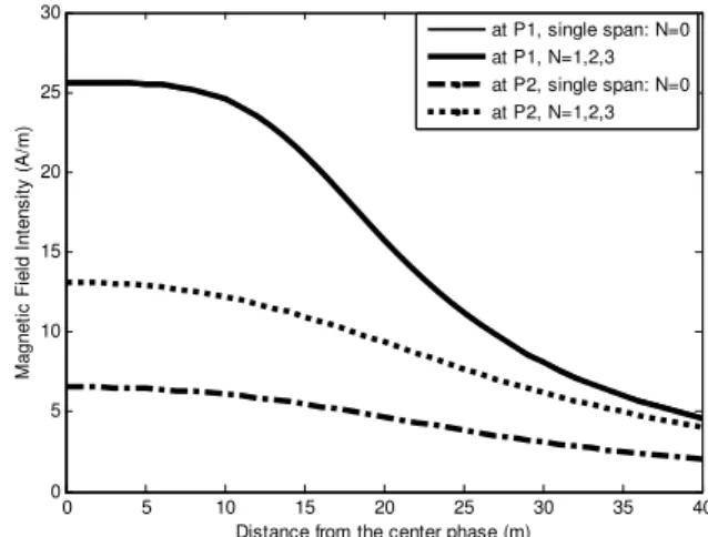
kA (24)Fig. (2) shows the effect of the number of spans (N) on the calculated magnetic field intensity. It is noticed that, when the magnetic field intensity calculated at point P1 (Fig.1) and a distance away from the center phase, the effect of the spans' number is very small due to the symmetry of the spans around the calculation points, as explained in Fig. (1), where the contributions of the catenaries d1 and d2 are equal and smaller than the contribution of the catenary d, as they far from the field points. But when the magnetic field intensity calculated at point P2 (Fig.1) and a distance away from the center phase, the effect of the spans' number is of great effect (double), that due to the contribution of the catenary d2 which produced the same magnetic field intensity as the original span d in this case as explained in Fig. (1), and of course the catenary d1 have a small contribution in the calculated values of the magnetic field intensities in this case.
TABLE(II)
CHARACTERISTICS OF 500KVLINE CONDUCTORS
Conductor number
Radius (mm)
X- Coordinate
(m)
Y- Coordinate
(m)
Rdc at
20°C
(Ω/km)
1a 15.3 -13.425 22.13 0.0511
1b 15.3 -12.975 22.13 0.0511
1c 15.3 -13.2 21.74 0.0511
2a 15.3 -0.225 24.48 0.0511
2b 15.3 0.225 24.48 0.0511
2c 15.3 0 24.09 0.0511
3a 15.3 12.975 22.13 0.0511
3b 15.3 13.425 22.13 0.0511
3c 15.3 13.2 21.74 0.0511
G1 5.6 -8 30 0.564
G2 5.6 8 30 0.564
L1 11.2 -13.2 17 0.1168
L2 11.2 13.2 17 0.1168
Fig. (3) shows the effects of the temperatures on the configuration of overhead transmission line conductors (sag) and hence on the calculated magnetic field intensity by using 3D integration technique with MTL technique. It is seen that as the sag increased with the increase in the temperatures (as
indicated in table (I)), the magnetic field intensity also increased. Fig. (4) shows the comparison between the magnetic filed calculated with both 2D straight line technique where the average conductors' heights are used, and 3D integration technique with MTL technique. It is seen that the observed maximum error of -23.2959% ( at point P1) and 49.877% at (point P2) is mainly due to the negligence of the sage effect on the conductors.
Fig. 2. The effect of the spans' numbers on the magnetic field intensity.
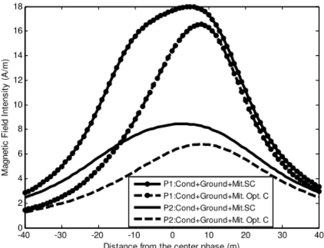
Fig. (5) shows the comparison between the magnetic field intensity calculated by using 3D integration technique with MTL technique with and without ground wires and with and without the short circuit mitigation loop. It is seen that, the observed maximum reduction of 1.9316% (at point P1) and 2.469% (at point P2) is mainly due to the negligence of the ground wires. It is seen that with the short circuit mitigation loop placed 5m below beneath the outer phase conductors, the magnetic field intensity reduced to a significant values, maximum reduction of 25.7063% (at point P1) and 30.1525% (at point P2). The magnetic field intensity can be reduced further by inserting an appropriately chosen series capacitor in the mitigation loop, in order to determine the optimal capacitance Cs of the capacitor to be inserted in the mitigation loop, the magnetic field intensity calculated at point one meter above ground surface under center phase, considering different values of Zc where Zc=jXs, with the reactance Xs varies from -2Ω to 0.
Fig. 3. The effect of the temperatures on the magnetic field intensity.
0 5 10 15 20 25 30 35 40 0
5 10 15 20 25 30
Distance from the center phase (m)
M
agne
ti
c
F
ie
ld I
nt
ens
it
y
(
A
/m
)
at P1, single span: N=0 at P1, N=1,2,3 at P2, single span: N=0 at P2, N=1,2,3
0 5 10 15 20 25 30 35 40 0
5 10 15 20 25 30
Distance from the center phase (m)
M
agne
ti
c
F
ie
ld I
nt
ens
it
y
(
A
/m
)
Fig. 4. Comparison between the 2D average heights and 3D integration technique results.
Fig. (6) shows the graphical results of the effect of the reactance Xs, inserted in the mitigation loop, on the magnetic field intensity, from which it is seen that the optimal situation (minimum value of magnetic field intensity) is characterized by Cs=4.897mF, and worst situation (maximum value of magnetic field intensity) is characterizes by Cs=2.358 mF.
Fig. 5. Comparison between the calculated magnetic field intensity values result from the conductors only, the conductors and ground wires, and the conductors, ground wires and short circuit mitigation loop.
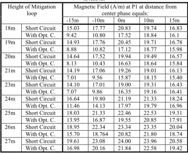
Tables (III) and (IV) depict the effect of the mitigation loop height on the calculated magnetic field intensity at points P1 and P2, respectively, when the mitigation loop spacing is 26.4m (exactly under the outer phases). It is seen that the optimal height is one meter below the outer phase conductors when the mitigation loop is short circuited and about one meter above the outer phase conductors when an optimal capacitance inserted in the mitigation loop. Tables (V) and (VI) depict the effect of the mitigation loop spacing on the calculated magnetic field intensity at points P1 and P2, respectively, when the mitigation loop height is 21m. It is seen that the optimal spacing is the outer phase conductors spacing. Figure (7) shows the comparison between the calculated magnetic field intensity values result from; the conductors, ground wires and short circuit mitigation loop; and the conductors, ground wires and mitigation loop with optimal capacitance and optimal parameters obtained from tables (III), (IV), (V) and (VI). It is seen that the magnetic
field intensity decreased further more, maximum reduction of 8.0552% (at point P1) and 19.5326% (at point P2).
Fig. 6. The effect of the reactance Xs, inserted in the mitigation loop, on the magnetic field intensity.
TABLE(III)
THE EFFECT OF THE MITIGATION LOOP HEIGHTS ON THE CALCULATED MAGNETIC FIELD INTENSITY AT POINT (P1) AND 26.4M MITIGATION LOOP
SPACING. Height of Mitigation
loop
Magnetic Field (A/m) at P1 at distance from center phase equals:
-15m -10m 0m 10m 15m
18m Short Circuit 15.03 17.77 20.83 19.74 16.83
With Opt. C. 9.42 10.80 17.52 18.84 16.1
19m Short Circuit 14.93 17.76 20.45 19.71 16.78
With Opt. C. 8.88 10.82 17.12 18.77 15.98
20m Short Circuit 14.64 17.52 19.94 19.49 16.57
With Opt. C. 8.13 10.43 16.63 18.64 15.84
21m Short Circuit 14.19 17.06 19.26 19.01 16.13
With Opt. C. 7.01 9.56 15.87 18.15 15.40
23m Short Circuit 14.10 17.01 19.00 19.31 16.43
With Opt. C. 7.07 9.86 16.35 19.16 16.41
24m Short Circuit 16.64 19.80 21.19 21.33 18.24
With Opt. C. 11.46 14.13 17.97 19.79 16.96
25m Short Circuit 18.03 21.33 22.46 22.53 19.31
With Opt. C. 13.95 16.87 19.55 20.85 17.91
26m Short Circuit 18.95 22.34 23.34 23.35 20.04
With Opt. C. 15.70 18.764 20.82 21.80 18.74
27m Short Circuit 19.61 23.08 24.00 23.96 20.58
With Opt. C. 16.98 20.16 21.84 22.58 19.42
TABLE(IV)
THE EFFECT OF THE MITIGATION LOOP HEIGHTS ON THE CALCULATED MAGNETIC FIELD INTENSITY AT POINT (P2) AND 26.4M MITIGATION LOOP
SPACING. Height of Mitigation
loop
Magnetic Field (A/m) at P2 at distance from center phase equals:
-15m -10m 0m 10m 15m
18m Short Circuit 7.97 8.89 9.88 9.43 8.61
With Opt. C. 5.49 6.28 7.77 7.99 7.44
19m Short Circuit 7.77 8.7 9.68 9.26 8.44
With Opt. C. 5.15 5.98 7.53 7.85 7.30
20m Short Circuit 7.48 8.4 9.37 9.00 8.20
With Opt. C. 4.67 5.54 7.21 7.64 7.12
21m Short Circuit 7.09 7.99 8.93 8.61 7.84
With Opt. C. 3.98 4.88 6.67 7.25 6.76
23m Short Circuit 6.79 7.71 8.72 8.49 7.72
With Opt. C. 3.91 4.93 6.98 7.72 7.22
24m Short Circuit 8.06 9.09 10.06 9.65 8.74
With Opt. C. 5.52 6.49 8.01 8.30 7.66
25m Short Circuit 8.76 9.85 10.82 10.32 9.33
With Opt. C. 6.67 7.68 8.99 9.01 8.25
26m Short Circuit 9.23 10.37 11.34 10.78 9.74
With Opt. C. 7.5 8.56 9.76 9.61 8.75
27m Short Circuit 9.58 10.75 11.73 11.13 10.05
With Opt. C. 8.13 9.22 10.37 10.09 9.17
0 5 10 15 20 25 30 35 40 0
5 10 15 20 25 30
Distance from the center phase (m)
M
a
gnet
ic
F
iel
d
I
nt
ens
it
y
(
A
/m
)
P1, at N=2 2D, Average Hights P2, at N=2
-40 -30 -20 -10 0 10 20 30 40 0
5 10 15 20 25 30
Distance from the center phase (m)
M
agne
ti
c
F
ie
ld I
nt
ens
it
y
(
A
/m
)
P1: Cond P1: Cond+Ground P1:Cond+Ground+Mit.SC P2: Cond P2: Cond+Ground P2:Cond+Ground+Mit.SC
-2 -1.8 -1.6 -1.4 -1.2 -1 -0.8 -0.6 -0.4 -0.2 0 5
10 15 20 25 30 35 40 45 50
Xs (Ohm)
M
agne
ti
c
F
ie
ld I
nt
ens
it
y
(
A
/m
)
Fig. 7. Comparison between the calculated magnetic field intensity values result from the conductors, ground wires and short circuit mitigation loop; and from the conductors, ground wires and mitigation loop with capacitance of optimal value at optimal height and spacing
TABLE(V)
THE EFFECT OF THE MITIGATION LOOP SPACINGS ON THE CALCULATED MAGNETIC FIELD INTENSITY AT POINT (P1) AND 21M HEIGHT. Distance of Mitigation
loop from the center phase
Magnetic Field (A/m) at P1 at distance from center phase equals:
-15m -10m 0m 10m 15m
5m Short Circuit 21.54 25.03 24.88 25.56 22.20
With Opt. C. 20.77 24.07 23.28 24.83 21.75
7.5m Short Circuit 20.43 23.48 23.24 24.15 21.22
With Opt. C. 18.65 21.21 20.67 22.73 20.26
10m Short Circuit 18.35 20.90 21.42 21.98 19.45
With Opt. C. 14.77 16.58 18.25 20.19 18.01
13.2m Short Circuit 14.19 17.06 19.26 19.01 16.13
With Opt. C. 7.01 9.56 15.87 18.15 15.40
15m Short Circuit 14.57 18.22 20.51 20.19 16.69
With Opt. C. 7.66 11.28 17.14 19.17 16.12
TABLE(VI)
THE EFFECT OF THE MITIGATION LOOP SPACINGS ON THE CALCULATED MAGNETIC FIELD INTENSITY AT POINT (P2) AND 21M HEIGHT. Distance of Mitigation
loop from the center phase
Magnetic Field (A/m) at P2 at distance from center phase equals:
-15m -10m 0m 10m 15m
5m Short Circuit 10.69 11.89 12.79 12.17 11.06
With Opt. C. 10.21 11.32 12.16 11.73 10.72
7.5m Short Circuit 10.06 11.14 11.96 11.46 10.47
With Opt. C. 9.01 9.94 10.73 10.57 9.77
10m Short Circuit 9.01 9.97 10.77 10.38 9.52
With Opt. C. 7.13 7.93 8.91 9.05 8.44
13.2 m
Short Circuit 7.09 7.99 8.93 8.61 7.84
With Opt. C. 3.98 4.88 6.67 7.25 6.76
15m Short Circuit 7.28 8.33 9.41 8.98 8.08
With Opt. C. 4.34 5.38 7.24 7.69 7.10
V. CONCLUSIONS
Ordinary simplifications, which usually are assuming, in the calculation of the magnetic field under overhead transmission lines, actually result in a model where magnetic fields are distorted from those produced in reality. These simplifications include neglecting the earth currents, neglecting the ground wires, replacing bundle phase conductors with equivalent single conductor, and replacing actual sagged conductors with average height horizontal conductors.
In this paper, the effects of the currents in the subconductors of each phase bundle, the currents in the ground wires, the currents in the mitigation loop, and also the earth return currents; in the calculation of the magnetic field under the 500kV Egyptian overhead transmission line, are investigated by using the MTL technique. Furthermore, the effect of the conductor’s sag between towers, and the effect of sag variation with the temperature on the calculated magnetic field is studied. The results from this method without mitigation loop are compared with those produced from the common practice 2-D method.
Finally the passive loop conductor design parameters, for Egyptian 500kV overhead transmission line, are obtained at ambient temperature (35oC).
REFERENCES
[1] Ahmed A. Hossam-Eldin, "Effect of Electromagnetics Fields from
Power Lines on Living Organisms" 2001 IEEE 7th International
Conference on Solid Dielectrics, June 25-29, Eindhoven, the Netherlands , pp. 438-441
[2] H. Karawia, K. Youssef and A. A. Hossam-Eldin "Measurements and
Evaluation of Adverse Health Effects of Electromagnetic Fields from Low Voltage Equipments" MEPCON 2008, Aswan, Egypt, March 12-15 ,PP. 436-440.
[3] A. A. Dahab, F. K. Amoura, and W. S. Abu-Elhaija "Comparison of
Magnetic-Field Distribution of Noncompact and Compact Parallel Transmission-Line Configurations" IEEE Transactions on Power Delivery, Vol. 20, No. 3, pp. 2114-2118, July 2005.
[4] J. R. Stewart, S. J. Dale, K. W. Klein "Magnetic Field Reduction
Using High Phase order Lines" IEEE Transactions on Power Delivery, Vol. 8, No. 2, April 1993, pp. 628-636.
[5] K. Yamazaki, T. Kawamoto, and H. Fujinami "Requirements for
Power Line Magnetic Field Mitigation Using a Passive Loop Conductor" IEEE Transactions on Power Delivery, Vol. 15, No. 2, April 2000, pp. 646-651
[6] R. G. Olsen and P. Wong, “Characteristics of low frequency electric
and magnetic fields in the vicinity of electric power lines” IEEE Transactions on Power Delivery, Vol. 7, No. 4, October 1992, pp. 2046-2053.
[7] R. D. Begamudre,”Extra High Voltage AC. Transmission
Engineering” third Edition, Book, Chapter 7, pp.172-205, 2006 Wiley Eastern Limited.
[8] J. A. Brandão Faria, and M. E. Almeida "Accurate Calculation of
Magnetic-Field Intensity Due to Overhead Power Lines With or Without Mitigation Loops With or Without Capacitor Compensation" IEEE Transactions on Power Delivery, Vol. 22, No. 2, April 2007, pp. 951-959
[9] W. de Villiers, J. H. Cloete, L. M. Wedepohl, and A. Burger
"Real-Time Sag Monitoring System for High-Voltage Overhead Transmission Lines Based on Power-Line Carrier Signal Behavior" IEEE Transactions on Power Delivery, Vol. 23, No. 1, January 2008, pp. 389-395
[10] T. Noda,"A Double Logarithmic Approximation of Carson’s
Ground-Return Impedance", IEEE Transactions on Power Delivery, Vol. 21, No. 1, January 2005, pp. 472-479
[11] A. Ramirez, and F. Uribe," A Broad Range Algorithm for the
Evaluation of Carson’s Integral", IEEE Transactions on Power Delivery, Vol. 22, No. 2, April 2007, pp. 1188-1193
[12] R. Benato, and R. Caldon," Distribution Line Carrier: Analysis
Procedure and Applications to DG", IEEE Transactions on Power Delivery, Vol. 22, No. 1, January 2007, pp. 575-583
[13] Adel Z. El Dein, "Magnetic Field Calculation under EHV
Transmission Lines for More Realistic Cases", IEEE Transactions on Power Delivery, Vol. 24, No. 4, pp. 2214-2222, October 2009.
[14] A. V. Mamishev, R. D. Nevels, and B. D. Russell "Effects of
Conductor Sag on Spatial Distribution of Power Line Magnetic Field" IEEE Transactions on Power Delivery, Vol.11, No.3, pp.1571-1576, July 1996.
[15] http://infocom.cqu.edu.au/Staff/Michael_O_malley/web/overhead_cab
le_sag_calculator.html.
-40 -30 -20 -10 0 10 20 30 40 0
2 4 6 8 10 12 14 16 18
Distance from the center phase (m)
M
a
gnet
ic
F
iel
d
I
nt
ens
it
y
(
A
/m
)