❊♥s❛✐♦s ❊❝♦♥ô♠✐❝♦s
❊s❝♦❧❛ ❞❡ Pós✲●r❛❞✉❛çã♦ ❡♠ ❊❝♦♥♦♠✐❛ ❞❛ ❋✉♥❞❛çã♦ ●❡t✉❧✐♦ ❱❛r❣❛s
◆◦ ✻✽✷ ■❙❙◆ ✵✶✵✹✲✽✾✶✵
❚❡st✐♥❣ t❤❡ ❖♣t✐♠❛❧✐t② ♦❢ ❆❣❣r❡❣❛t❡ ❈♦♥✲
s✉♠♣t✐♦♥ ❉❡❝✐s✐♦♥s✿ ■s t❤❡r❡ ❘✉❧❡✲♦❢✲❚❤✉♠❜
❇❡❤❛✈✐♦r❄
❋á❜✐♦ ❆✉❣✉st♦ ❘❡✐s ●♦♠❡s✱ ❏♦ã♦ ❱✐❝t♦r ■ss❧❡r
❖s ❛rt✐❣♦s ♣✉❜❧✐❝❛❞♦s sã♦ ❞❡ ✐♥t❡✐r❛ r❡s♣♦♥s❛❜✐❧✐❞❛❞❡ ❞❡ s❡✉s ❛✉t♦r❡s✳ ❆s
♦♣✐♥✐õ❡s ♥❡❧❡s ❡♠✐t✐❞❛s ♥ã♦ ❡①♣r✐♠❡♠✱ ♥❡❝❡ss❛r✐❛♠❡♥t❡✱ ♦ ♣♦♥t♦ ❞❡ ✈✐st❛ ❞❛
❋✉♥❞❛çã♦ ●❡t✉❧✐♦ ❱❛r❣❛s✳
❊❙❈❖▲❆ ❉❊ PÓ❙✲●❘❆❉❯❆➬➹❖ ❊▼ ❊❈❖◆❖▼■❆ ❉✐r❡t♦r ●❡r❛❧✿ ❘❡♥❛t♦ ❋r❛❣❡❧❧✐ ❈❛r❞♦s♦
❉✐r❡t♦r ❞❡ ❊♥s✐♥♦✿ ▲✉✐s ❍❡♥r✐q✉❡ ❇❡rt♦❧✐♥♦ ❇r❛✐❞♦ ❉✐r❡t♦r ❞❡ P❡sq✉✐s❛✿ ❏♦ã♦ ❱✐❝t♦r ■ss❧❡r
❉✐r❡t♦r ❞❡ P✉❜❧✐❝❛çõ❡s ❈✐❡♥tí✜❝❛s✿ ❘✐❝❛r❞♦ ❞❡ ❖❧✐✈❡✐r❛ ❈❛✈❛❧❝❛♥t✐
❆✉❣✉st♦ ❘❡✐s ●♦♠❡s✱ ❋á❜✐♦
❚❡st✐♥❣ t❤❡ ❖♣t✐♠❛❧✐t② ♦❢ ❆❣❣r❡❣❛t❡ ❈♦♥s✉♠♣t✐♦♥ ❉❡❝✐s✐♦♥s✿ ■s t❤❡r❡ ❘✉❧❡✲♦❢✲❚❤✉♠❜ ❇❡❤❛✈✐♦r❄✴
❋á❜✐♦ ❆✉❣✉st♦ ❘❡✐s ●♦♠❡s✱ ❏♦ã♦ ❱✐❝t♦r ■ss❧❡r ✕ ❘✐♦ ❞❡ ❏❛♥❡✐r♦ ✿ ❋●❱✱❊P●❊✱ ✷✵✶✵
✭❊♥s❛✐♦s ❊❝♦♥ô♠✐❝♦s❀ ✻✽✷✮
■♥❝❧✉✐ ❜✐❜❧✐♦❣r❛❢✐❛✳
Testing the Optimality of Aggregate Consumption
Decisions: Is there Rule-of-Thumb Behavior?
Fábio Augusto Reis Gomes
IBMEC-SP
Rua Quatá, 300
São Paulo, SP 04546-042
Brazil
[email protected]
João Victor Issler
yGraduate School of Economics – EPGE
Getulio Vargas Foundation
Praia de Botafogo 190 s. 1100
Rio de Janeiro, RJ 22250-900
Brazil
[email protected]
February, 2009.
Keywords: Optimal Consumption, Consumption Rule-of-Thumb,
Intertemporal Substitution, Euler-Equation Aggregation, Aggregate
Abstract
Consumption is an important macroeconomic aggregate, being about 70% of GNP.
Finding sub-optimal behavior in consumption decisions casts a serious doubt on whether
optimizing behavior is applicable on an economy-wide scale, which, in turn, challenge
whether it is applicable at all.
This paper has several contributions to the literature on consumption optimality.
First, we provide a new result on the basic rule-of-thumb regression, showing that it is
observational equivalent to the one obtained in a well known optimizing
real-business-cycle model. Second, for rule-of-thumb tests based on the Asset-Pricing Equation, we
show that the omission of the higher-order term in the log-linear approximation yields
inconsistent estimates when lagged observables are used as instruments. However,
these are exactly the instruments that have been traditionally used in this literature.
Third, we show that nonlinear estimation of a system of N Asset-Pricing Equations
can be done e¢ciently even if the number of asset returns (N) is high vis-a-vis the
number of time-series observations (T). We argue that e¢ciency can be restored by
aggregating returns into a single measure that fully captures intertemporal substitution.
Indeed, we show that there is no reason why return aggregation cannot be performed
We are especially grateful to Caio Almeida, Marco Bonomo, Luis Braido, Carlos E. Costa, Pedro C. Ferreira, Naércio A. Menezes Filho, for their comments and suggestions of improvement on earlier versions of this paper. We also bene…ted from comments given by the participants of the conferences SBE 2005, SBFIN 2006, and the Econometric Society Meetings of Vienna and of Mexico City, where this paper was presented. The usual disclaimer applies. Fabio Augusto Reis Gomes and João Victor Issler gratefully acknowledge support given by CNPq-Brazil. Issler also ackowledges the support given by CAPES, Pronex and FAPERJ.
in the nonlinear setting of the Pricing Equation, since the latter is a linear function
of individual returns. This forms the basis of a new test of rule-of-thumb behavior,
which can be viewed as testing for the importance of rule-of-thumb consumers when the
optimizing agent holds an equally-weighted portfolio or a weighted portfolio of traded
assets.
Using our setup, we …nd no signs of either rule-of-thumb behavior for U.S.
con-sumers or of habit-formation in consumption decisions in econometric tests. Indeed,
we show that the simple representative agent model with a CRRA utility is able to
explain the time series data on consumption and aggregate returns. There, the
in-tertemporal discount factor is signi…cant and ranges from 0:956 to 0:969 while the
relative risk-aversion coe¢cient is precisely estimated ranging from 0:829 to 1:126.
There is no evidence of rejection in over-identifying-restriction tests.
1
Introduction
For the U.S. economy, there has been a large early literature using time-series data
reject-ing optimizreject-ing behavior in consumption generatreject-ing some relevant puzzles; see Hall (1978),
Flavin (1981), Mankiw (1981), Hansen and Singleton (1982, 1983, 1984), Mehra and Prescott
(1985), and Campbell and Deaton (1989). In two in‡uential articles, following an initial idea
in Hall and Mishkin (1982), Campbell and Mankiw (1989, 1990) extended the basic
opti-mizing model incorporating rule-of-thumb behavior. There are two types of consumers: the
…rst type consumes according to optimizing behavior but the second consumes only his/her
current income. In this context, tests of no rule-of-thumb behavior are performed using the
data, Campbell and Mankiw concluded that rule-of-thumb behavior was widespread. For
the U.S. economy, about 50% of total income belongs to rule-of-thumb consumers. Evidence
for other countries are even more “compelling.”
In econometric tests, whenever a speci…c null hypothesis is being tested, there are usually
auxiliary hypothesis being tested as well. In Campbell and Mankiw’s case, when testing for
the nonexistence of rule-of-thumb consumers, the auxiliary assumption is the validity of the
…rst-order log-linearized version of the euler equation for optimizing consumers. Rejecting
the null may be due to the inappropriateness of optimizing behavior or to the fact that the
…rst-order log-linear approximation of the euler equation is a poor one (or both).
In this paper, we o¤er theoretical and econometric reasons to invalidate empirical results
of current rule-of-thumb tests, showing that rule of thumb is not present when novel
empir-ical tests are applied to U.S. data. First, using the dynamic stochastic general-equilibrium
(DSGE) model of King, Plosser and Rebelo (1988), with no rule-of-thumb behavior, Issler
and Vahid (2001) showed that there exists a linear combination of consumption and income
growth that is unpredictable. This is exactly the implication that basic rule-of-thumb tests
investigates. Observational equivalence implies that, even if one …nds that income and
con-sumption growth have similar short-run co-movement, one cannot conclude in favor of the
presence of rule-of-thumb. Second, employing a generalized taylor expansion of the
opti-mizing consumer’s euler equation, we consider what are the econometric consequences of
ignoring high-order terms once a naïve …rst-order expansion is …tted to data. As one should
expect, ignoring higher-order terms yields inconsistent estimates of the proportion of
rule-of-thumb consumers, invalidating hypothesis testing. Third, as is well known, this …rst-order
on consumption, income and the return to aggregate capital, we provide evidence that these
stringent restrictions are not valid. Moreover, when an appropriate novel rule-of-thumb test
is applied to this same data set, we …nd no evidence of its presence.
The possibility of a positive bias for the proportion of rule-of-thumb consumers in current
tests was discussed by Weber (2002). He follows Cushing (1992), who argues that the
combination of quadratic utility with habit formation implies that observed consumption
growth is correctly modeled as a …rst order autoregressive-distributed lag function of growth
in disposable income. Omission of this term in rule-of-thumb tests leads to a positive bias for
the proportion of rule-of-thumb consumers, since lagged income variation is highly positively
correlated with the error term. This explains the large presence of rule-of-thumb consumers
found by Campbell and Mankiw and in the literature that followed. A crucial step in Weber’s
result is to assume that habit formation is present in preferences.
Here we go one step further by using a generalized taylor expansion approach. Regardless
of the way one speci…es preferences, unless the highly restrictive assumption that
consump-tion growth and asset returns are log-Normal and homoskedastic is kept, we show that,
once higher-order terms are omitted in running rule-of-thumb tests, all lagged observables
are invalid instruments in log-linear regressions. But these are exactly the instruments that
have been used in testing rule-of-thumb behavior up to now. Moreover, it is hard to …nd
instruments other than lagged observables. Hence, our critique is much deeper than that of
Weber’s.
Once we fully characterized the problem, we searched for a robust test for the existence
of rule-of-thumb consumers. As in Weber, we …rst employ the nonlinear euler equation as a
is aggregate consumption minus rule-of-thumb consumption. Thus, we can write the euler
equation of the optimizing consumer in terms of observables and unknown parameters, and
the generalized method-of-moments (GMM) can be used in estimation and as a basis for
testing. Second, we argue that the e¢cient estimation of intertemporal substitution requires
the use of all assets in the economy. This is a consequence of the fact that the Asset-Pricing
Equation is valid for all traded securities and not for just a few. In other words, consumption
should only respond to systematic changes in returns and individual returns can ‡uctuate
because of idiosyncratic changes. Because it may be unfeasible to use all asset returns in
the economy – if the number of time-observations is relatively small vis-a-vis the number
of assets – we propose the cross-sectional aggregation of the nonlinear euler equation of
individual returns, showing that the resulting aggregate equation can be viewed as the euler
equation for the optimizing agent when he/she holds an equally-weighted portfolio of traded
assets (or a weighted portfolio). In this context, aggregation is optimal, which follows from
the work of Driscoll and Kraay (1998).
In a log-linear setting, the idea that the cross-sectional aggregation of individual returns
follows closely intertemporal substitution was the key insight of Mulligan (2002). Here, we
go one step further and show that we can perform cross-sectional aggregation of the euler
equation for individual returns. This is feasible, interpretable, and also e¢cient when the
number of cross-sectional units grows large, as argued in Driscroll and Kraay.
Attanasio and Weber (1995) show that the euler equation of an individual consumer is
nonlinear on consumption. Therefore, aggregating euler equations across consumers using
the techniques in Browning, Deaton and Irish (1985) and Deaton (1985) does not yield the
cross-sectionally aggregated across returns, since they are a linear function of individual returns.
The aggregate euler equation will be that of a representative consumer who holds an
equally-weighted portfolio of traded assets (or a equally-weighted portfolio).
Empirically, we provide overwhelming evidence against rule-of-thumb behavior for U.S.
consumers and against habit-formation in consumer preferences using novel tests. Our results
are in sharp contrast to those in Campbell and Mankiw regarding rule of thumb and to those
in Weber regarding habit formation. Indeed, we show that we can appropriately represent
preferences for the U.S. consumer using a constant relative-risk-aversion (CRRA) utility
function: estimates of the annual discount factor are signi…cant and range from 0:956 to
0:969, while those of the relative risk-aversion coe¢cient are also signi…cant ranging from
0:829 to 1:126. Moreover, there is no evidence of rejection in over-identifying-restriction tests.
Our key result is that, once proper models and econometric techniques are applied to
aggregate consumption, income, and aggregate return data, there is no reason to challenge
optimizing behavior in consumption, as was the case with previous rule-of-thumb tests. We
also show that augmented models for preferences such as consumption with habit
forma-tion are unnecessary to characterize intertemporal substituforma-tion. In that sense, our evidence
reduces the fear that optimizing behavior is the exception, not the rule.
The paper proceeds as follow. Section 2 presents the problem and our proposed solution.
2
Testing Rule-of-Thumb Behavior in Consumption
2.1
The Standard Approach
The initial idea about rule-of-thumb behavior in consumption was proposed by Hall
and Mishkin (1982) in a panel-data context. Campbell and Mankiw (1989, 1990) extended
their setup making it operational using time-series techniques: interpreting aggregate
regres-sion coe¢cients and providing an econometric test for its presence at the aggregate level.
Campbell and Mankiw have a basic restrictive framework, where optimizing consumers have
quadratic utility, and a more general setup where optimizing behavior is consistent with the
Asset Pricing Equation, albeit subject to the validity of a log-linear approximation.
Campbell and Mankiw’s basic framework has two types of consumers: consumer of the
…rst type (consumer 1) consumes according to optimizing behavior under quadratic utility. They impose Hall’s (1978) restriction that the product of the discount rate and the
one-period real return on wealth is equal to unity in every one-period, leading to the result that
consumption of the optimizing agent is a martingale1. The second type of consumer is
restricted to consume his/her current income(Y2;t), with no optimizing behavior. Income of
the restricted consumer holds a …xed proportion( )to aggregate income as follows: = Y2;t
Yt ,
leading to the following relationship between aggregate consumption(Ct) and income(Yt):
Ct= + Yt+ (1 ) t, (1) 1Alternatively, we can think of the optimizing agent following the permanent-income framework as
or, to a logarithmic approximation:
ln (Ct) = + ln (Yt) + (1 ) t; (2)
where t is unpredictable, since it is an innovation regarding the optimizing agent’s
informa-tion set.
Because the framework of quadratic utility is too restrictive, Campbell and Mankiw
expanded their basic framework to deal with the (Asset) Pricing Equation, using an aggregate
return to wealth(Rt+1):
Et
u0
(Ct+1)
u0(C
t)
Rt+1 = 1; (3)
where Et( ) denotes the conditional expectation given the information available at time t,
u0
( ) > 0 is the …rst derivative of the utility function, and 2 (0;1). Under the same structure as before – one optimizing agent whose consumption obeys (3) and one restricted
agent whose consumption equals Yt – they obtain:
ln (Ct) = ln (Yt) + (1 )
1
ln ( ) + 2
2 + 1r
t + t, (4)
where it is assumed that u0
(Ct) = Ct , with representing the constant relative
risk-aversion coe¢cient, and rt = ln (Rt). Again, the error term t is unpredictable, since it is
an innovation regarding the optimizing agent’s information set.
Testing the presence of rule-of-thumb behavior in consumption amounts to a statistical
test of the null hypothesis H0 : = 0either in (2) or in (4), where estimation is done using instrumental-variable techniques. Under H0, non-optimizing consumers have zero income
and are therefore negligible.
The conditions under which equations (1) (or (2)) and (4) are derived are very stringent.
other hand, log-linearizing (3) leading to (4) requires joint conditional log-Normality and
homoskedasticity of Ct
Ct 1; Rt
0
, yielding:
ln (Ct) =
1
ln ( ) + 2
2 + 1r
t+ t, (5)
where tj t 1 N 0; 2 , with t 1 representing the information set of the optimizing agent.
The fact that t is conditionally Gaussian and uncorrelated with elements of the
con-ditioning set t 1 implies that t and t s, s > 0 are independent. Moreover, t must be
independent of any function of the variables in t 1. In principle, residual-based tests of
normality, conditional homoskedasticity, and independence can be used to ensure that these
restrictions apply to t. In particular, we employ the Jarque and Bera (1987) test for normal
errors, the LM serial correlation test, the ARCH test for homoskedasticity, and the Brock et
al.’s (1996) BDS test for independence.
2.2
Observational Equivalence: A Critique of the Basic Model
Testing Rule-of-Thumb
As stressed in Issler and Vahid (2001), in the dynamic stochastic general equilibrium
(DSGE) model of King, Plosser, and Rebelo (1988), output, consumption and investment
share co-movements (or have common features) as a result of the optimizing behavior of
the representative agent. Under log-utility, full-depreciation of the capital stock, and
consumption(Ct), and investment (It), are, respectively:
log (Yt) = log (Xtp) +y+ ykkbt
log (Ct) = log (Xtp) +c+ ckkbt
log (It) = log (Xtp) +i+ ikkbt; (6)
wherelog (Xtp) = + log X p t 1 +"
p
t is the random-walk productivity process,y,candi are
the steady-state values of log (Yt=X p
t); log (Ct=X p
t), and log (It=X p
t) respectively, and jk;
j = y; c; i is the elasticity of variable j with respect to deviations of the capital stock from its stationary value kbt .
Focusing on the …rst two equations in (6), it is straightforward to verify that:
log (Ct) = ck
yk
log (Yt) +
ck yk
yk
( +"pt): (7)
where "pt is the innovation of the productivity processlog (X p t).
Recall now the basic setup with quadratic utility in Campbell and Mankiw (1989, 1990),
represented by equation (2). It is straightforward to conclude that (7) and (2) are
observa-tionally equivalent, with ck yk = ,
ck yk
yk = , and
ck yk
yk
p
t = (1 ) t. Thus, validating
(2) with data cannot be used to support the existence of rule-of-thumb behavior, since it
2.3
A Generalized Taylor-Expansion Approach:
A Critique of
Usual Log-Linear Approximations of the Asset-Pricing
Equa-tion Applied to Rule-of-Thumb Tests
The starting point of our approach is the Asset-Pricing Equation (or Pricing Equation,
for short):
EtfMt+1xi;t+1g=pi;t; i= 1;2; : : : ; N; or (8)
EtfMt+1Ri;t+1g= 1; i= 1;2; : : : ; N; (9)
where Mt is the stochastic discount factor, pi;t denotes the price of the i-th asset at time t,
xi;t+1 denotes the payo¤ of the i-th asset in t+ 1, Ri;t+1 = xi;tpi;t+1 denotes the gross return of thei-th asset in t+ 1, and N is the number of assets in the economy.
We assume that the Pricing Equation (9) holds and that the stochastic discount factor
obeys Mt =
u0(Ct)
u0(Ct 1) > 0, where 2 (0;1), and u
0
( ) > 0 is consumption’s marginal utility. Following Araujo and Issler (2008), we consider a generalized taylor expansion of the
exponential function aroundx; with incrementh; as follows:
ex+h =ex+hex+ h
2ex+ (h)h
2 ; with (h) :R!(0;1): (10)
For the expansion of a generic function, ( ) would depend on x and h. However, dividing (10) byex:
eh = 1 +h+ h
2e (h)h
2 ; (11)
function of h alone2.
To connect (11) with the Pricing Equation (9), we let h= ln(MtRi;t)to obtain:
MtRi;t = 1 + ln(MtRi;t) +
[ln(MtRi;t)]2e (ln(MtRi;t)) ln(MtRi;t)
2 : (12)
It is important to stress that (12) is not an approximation but an exact relationship. The
behavior of MtRi;t is governed solely by that of ln(MtRi;t). It is useful to de…ne a random
variable collecting the higher-order term in (12):
zi;t
1
2 [ln(MtRi;t)]
2
e (ln(MtRi;t)) ln(MtRi;t):
Notice that zi;t is a function of ln(MtRi;t) alone and that zi;t 0 for all (i; t). Taking the
conditional expectation of both sides of (12), imposing the Pricing Equation and rearranging
terms gives:
Et 1(zi;t) = Et 1fln(MtRi;t)g: (13)
To ensure that Et 1(zi;t) exists we constrain the process fln(MtRi;t)g so that its
condi-tional expectation is well de…ned. Weak-stationarity offln(MtRi;t)gis a su¢cient condition
for that. Let "t ("1;t; "2;t; :::; "N;t)0 stack the conditional mean of the individual forecast
errors "i;t = ln(MtRi;t) Et 1fln(MtRi;t)g. From the de…nition of "t we have:
ln(MtRt) =Et 1fln(MtRt)g+"t: (14)
Starting with (14), denoting ri;t = ln (Ri;t), mt = ln (Mt), and using Et 1(zi;t) = 2This solution is:
(h) =
8 > > < > > :
1
h ln
2 (eh 1 h)
h2 ; h6= 0
Et 1fln(MtRi;t)g, we get:
ri;t = mt Et 1(zi;t) +"i;t; i= 1;2; : : : ; N: (15)
Within a CCAPM framework, we specialize lettingu(Ct) =
Ct1 1
1 , for 6= 1, and u(Ct) =
ln (Ct), for = 1, i.e., the canonical form foru(Ct), which gives,
ln (Ct) =
ln ( )
+ 1ri;t+ E
t 1(zi;t)
+ i;t; i= 1;2; : : : ; N, (16)
where i;t = "i;t
.
It is important to stress that Et 1(zi;t)
captures the e¤ect of the higher-order terms of the
taylor expansion, in general it will be a function of the variables in the conditioning set used
by the econometrician to computeEt 1( ). Therefore, omission of Et 1(zi;t) (or of parts of it) in estimating (16) will generate an omitted-variable bias. This will turn out to be a major
problem for versions of (16) usually estimated in the rule-of-thumb literature3.
Using (16), we can write:
ln (Ct) =
(1 )
ln ( ) + ln (Yt) +
(1 )
ri;t (17)
+(1 )Et 1(zi;t) + (1 ) i;t, for all i
where the only di¤erence between (17) and Campbell and Mankiw’s setup (i.e., (4)) is the
inclusion of the term (1 )Et 1(zi;t) and the fact that we are considering N assets in the
economy instead of just one.
3
Notice that (16) is a generalized version of (5) when we consider several assets instead of just one. We do not impose any distributional assumptions on i;t and the higher order term E
t 1(zi;t) shows naturally in it.
When = 0, there is no rule-of-thumb behavior, therefore a critical issue in testing the null hypothesis H0 : = 0 is to obtain consistent estimates for . Suppose that the term
(1 )
Et 1(zi;t)is omitted in running (17). Then, the error term becomes correlated with all
the variables in the conditioning set used by the econometrician to computeEt 1(zi;t).
How-ever, these are the same variables used as instruments in past empirical studies. Within this
context, omitting (1 )Et 1(zi;t)results in inconsistent instrumental-variable (IV) estimates
for and invalid inference when testing H0 : = 0.
Notice that, in general, it is impossible to determine whether plim
T!1
dIV 70. However,
since most macroeconomic variables are pro-cyclical, it is very likely that plim
T!1
dIV >0
when (1 )Et 1(zi;t) is omitted, leading IV estimates to have an upward asymptotic bias,
explaining why so many macroeconomic studies rejected H0 : = 0 in favor of HA : >0;
see Campbell and Mankiw (1989) and most of the literature that followed.
Inconsistency of IV estimates is a result of omitting the term (1 )Et 1(zi;t) in running
(17). However, the only reason why this term is present in (17) is because we use a log-linear
approximation of the Pricing Equation (9). We can circumvent the problem if we do not try
to log-linearize the Pricing Equation. This was exactly the approach taken by Weber (2002),
who proposed an alternative way of testing rule-of-thumb behavior employing the non-linear
equation (9) directly. We must stress that Weber did not motivate his framework by using
the log-linearization argument employed here. We advance from Weber in the understanding
of the problem by considering the expansion (12). Because of that, we are able to show that
lagged observables are correlated with the error term due to omitted higher-order terms.
This is a much deeper critique of the rule-of-thumb approach in Campbell and Mankiw
observables as instruments, and omitted higher-order terms, their empirical …ndings may be
invalid.
Using a nonlinear instrumental variable estimator – a generalized method-of-moment
(GMM) estimator – Weber employed directly (9) to estimate structural parameters and test
H0 : = 0. He shows that we can write the optimizing agent’s consumption (C1;t) as a
function of observables since, under rule-of-thumb behavior:
C1;t =Ct Yt: (18)
Because the optimizing agent obeys the euler equation (9), we could use GMM to estimate
the structural parameters associated with the optimizing agent as well as in:
Et 1
u0
(Ct Yt)
u0(C
t 1 Yt 1)
Ri;t = 1; i= 1;2; : : : ; N; (19)
for a given choice ofu0
( ).
The only di¤erence between (19) and Weber’s setup is the fact that we are consideringN
assets in the economy instead of just one. We now try to justify the use of a disaggregated
setup for asset returns.
Most past empirical studies in consumption completely ignored the fact that the
opti-mizing agent decides on consumption when faced with the prospects of expected discounted
returns on N assets, such as in the system of equations in (19). E¢cient estimation of
pref-erence and other parameters in the system requires estimating the whole system instead of
just a portion of it. This happens for the same reason why single-equation OLS estimation
is less e¢cient than SUR estimation in the context of linear regressions. System estimation
N ! 1 with …xed T, estimating the whole system is unfeasible and full-e¢ciency cannot
be attained. Most of the literature opted to limit the size of N, e.g.,N = 2: a risky and a “riskless” asset or, at most, a handful of assets. Of course, this solution is sub-optimal at
the cost of e¢ciency.
In an interesting paper, Mulligan (2002) shows that an alternative to estimating the
system as a whole is cross-sectional aggregation, where we do not throw away useful
in-formation contained in Ri;t, i = 1;2; : : : ; N, but rather aggregate it to isolate the common
component of asset returns; see also the equivalent approach in Araujo and Issler (2008). The
idea behind cross-sectional aggregation is that intertemporal substitution is a consequence
of changes that a¤ect all returns, i.e., to systematic changes in returns, since idiosyncratic
movements inRi;t do not a¤ect aggregate consumption. IfN is su¢ciently large (orN ! 1)
cross-sectional aggregation will deliver the common component of returns associated with
intertemporal substitution.
As Campbell and Mankiw, Mulligan starts with a log-linear approximation of the Pricing
Equation (9) such as (16). In what follows we present a stylized version of Mulligan to be
able to discuss the problems related with approximating (9). Consider the sequence of
deterministic weights f!igNi=1, such that j!ij < 1 uniformly on N, with N
X
i=1
!i = 1 or
lim
N!1
N
X
i=1
!i = 1, depending on whether we allow or not the existence of an in…nite number
of assets. Cross-sectional aggregation of (16) implies:
ln (Ct) =
1
ln ( ) + 1rt+
1
Et 1(zt) + t, (20)
where rt = N
P
i=1
!iri;t is the logarithm of the return to the geometric average of aggregate
capital, zt = N
P
i=1
!izi;t, and t = N
P
i=1
use equal weights in aggregation. Despite aggregating returns, Mulligan omits the term
1
Et 1(zt) in estimating (20), potentially leading to an omitted-variable bias.
From an econometric point-of-view, the cross-sectional aggregation leading to (20) is very
similar to the theoretical approach of Driscoll and Kraay (1998), although the latter is more
general because it also applies if the setup is non-linear. They use orthogonality conditions
of the form E(h( ; wi;t)) = 0, i = 1;2; : : : ; N. If N is large relative to T, GMM estimation
is not feasible, since we cannot estimate consistently the variance-covariance matrix of the
sample moments. Despite that, since for allithe orthogonality conditions hold, we can form
a cross-sectional averageeh( ) = 1
N N
P
i=1
h( ; wi;t), and estimate by GMM fromE eh( ) = 0.
Under a set of standard assumptions, Driscoll and Kraay prove consistency and asymptotic
normality for the GMM estimates of . That happens whetherN is …xed orN ! 1 at any
rate. Here, despite specializing to !i = 1=N, cross-sectional aggregation is also the solution
to the problem of excess of orthogonality conditions.
It is important to stress that, although the approach in Mulligan is inappropriate if the
log-linear approximation of (9) is invalid, it is a clever way of preserving information on all
returns that would otherwise be lost if N is large relative toT.
In what follows, we show how to circumvent not only the problem of aggregation but
also the problem of using a log-linear approximation of (9). Start with a system of euler
equations for the unconstrained consumer (19):
Et 1
u0
(Ct Yt)
u0(C
t 1 Yt 1)
Ri;t = 1; i= 1;2; : : : ; N: (21)
k vector of instruments, dated int 1or before, common to all equations in (21). Centering (21), post-multiply the result byXt 1 and use the law of iterated expectations to achieve:
E u
0
(Ct Yt)
u0(C
t 1 Yt 1)
Ri;t 1 Xt 1 = 0; i= 1;2; : : : ; N: (22)
Label now:
h( ; wt; wi;t) =
u0
(Ct Yt)
u0(C
t 1 Yt 1)
Ri;t 1 Xt 1, i= 1;2; : : : ; N:
where the w’s denote data, and stacks , the preference parameters in u0
( ), and, more importantly, .
There are N k orthogonality conditions in (22). If N is large relative to T, estimating
the variance-covariance matrix of sample means will be infeasible, or poorly estimated, even
if it is feasible; see Driscoll and Kraay for a discussion of the latter. If we cross-sectionally
aggregate (22), we obtain:
e
h( ) = 1 N
N
X
i=1
h( ; wt; wi;t) =
u0
(Ct Yt)
u0(C
t 1 Yt 1)
Rt 1 Xt 1;
where Rt = N1 N
P
i=1
Ri;t is the cross-sectional average of all returns. Notice that we can still
estimate by GMM using:
E
n
eh( )o=E u
0
(Ct Yt)
u0(C
t 1 Yt 1)
Rt 1 Xt 1 = 0; (23)
but now we only have a system ofk orthogonality conditions, regardless of the size of N.
An interesting feature of this approach is that estimation is feasible without having to
throw away any information about asset returns. It works for any size of N and even if
N ! 1, at any rate. Moreover, the euler equation behind the moment restrictions in (23)
an equally-weighted portfolio of traded assets Rt = N1 N
P
i=1
Ri;t in every period. In a large N
environment, this return will beRt= plim N!1
1
N N
P
i=1
Ri;t. If we use deterministic weightsf!ig N i=1
in aggregating (22), as discussed above, then Rt = plim N!1
N
P
i=1
!iRi;t can be interpreted as a
weighted portfolio.
The way cross-section aggregation of returns works here is in sharp contrast with the
early literature on consumption aggregation of the euler equation; see Browning, Deaton
and Irish (1985), Deaton (1985) and Attanasio and Weber (1995). There, the problem lies
with the fact that uu0(0C(Ci;ti;t)1) is a nonlinear function of individual consumption Ci;t, which
generates an aggregation bias for euler equations estimated using aggregate consumptionCt.
Given a choice of u0
( ), we can estimate consistently the structural parameters in (23) and testH0 : = 0 by means of a simple wald test. This is exactly the approach taken here. In what follows, we employ two di¤erent speci…cations for preferences of the
uncon-strained agent in testing rule-of-thumb. The …rst is CRRA (or Power) utility, where:
u(C1;t) =
C11;t 1
1 =
(Ct Yt)1 1
1 : (24)
The second considers that the optimizing agent has external habit formation (Abel (1990)),
with u( )as follows:
u C1;t; C1;t 1 =
[(Ct Yt) (Ct 1 Yt 1)]1 1
1 ; (25)
where C1;t 1 is treated parametrically in the optimization problem.
The case where preferences are represented by (25) was studied by Weber. He did not
account by Weber. Indeed, he used the after-tax average yield on new issues of 6 month
Treasury bills. Since the marginal rate of substitution in consumption is only sensible to
systematic changes in real returns, and there is little reason for the real yield of the 6-month
Treasury bill to be a good proxy for these systematic changes, it is interesting to confront
the empirical results in Weber with the ones found here when a proxy forRt= N1 N
P
i=1
Ri;t or
Rt = N
P
i=1
!iRi;t is used instead. Indeed, Mulligan argues that “the interest rate in aggregate
theory is not the promised yield on a Treasury Bill or Bond, but should be measured as the
expected return on a representative piece of capital.”
The measure proposed by Mulligan is the return to aggregate capital Rt, or the capital
rental rate (after income and property taxes). To make the case for this measure as stark
as possible, we assume log-utility for preferences – where Mt+i = CCt+ti, i = 1;2; : : :, and
Mt= CCtt1 – as well as no production. Dividends are equal to consumption in every period,
and the price of the portfolio representing aggregate capital pt can be computed with the
usual expected present-value formula:
pt=Et
( 1
X
i=1
Mt+iCt+i
) =Et
( 1
X
i=1
i Ct
Ct+i
Ct+i
) =
1 Ct:
Hence, the return on aggregate capital Rt is given by:
Rt=
pt+Ct
pt 1
= Ct+ (1 )Ct Ct 1
= Ct Ct 1
= 1 Mt
; (26)
which is the reciprocal of Mt.
Equation (26) shows that changes in Rt are associated with intertemporal substitution.
However, changes in individual assets will only be associated with intertemporal substitution
3
Empirical Results
3.1
Data
The critical series used in this study is the capital rental rate after income and property
taxes, as computed in Mulligan (2002)4. This series was calculated in annual frequency, from
1947 to 1997. The rest of the data used were extracted from the U.S. National Income and
Product Account (NIPA) and from the US Census Bureau. From NIPA we extracted annual
data for real disposable personal income, real consumption of nondurable and services, and
real consumption of nondurables. To obtain per capita series we used population data from
the US Census Bureau.
3.2
Econometric Issues in GMM Estimation
As in any study employing GMM techniques it is important to choose instruments
prop-erly. Tauchen (1986), Mao (1990), and Fuhrer et al. (1995) have found that GMM performs
better with instrument sets including only a few lags of the observables in the equation being
estimated. As a general rule, we follow this strategy avoiding a weak-instrument problem.
Regardless whether we use (24) or (25) to represent preferences, we must guarantee that
the series in the euler equation are not integrated of order one. Since consumption and
income are known to have roots of the autoregressive polynomial equal (or nearly equal
to) to unity, we transform them to achieve stationarity within the euler equation. In the
context of rule-of-thumb tests, Weber (2002) discusses this issue at some length, dividing
euler equations by speci…c powers of Yt to generate non-integrated terms. These powers
depend on the form of preferences. Here, we opted for a slightly di¤erent route. For the
preferences in (24) or (25), dividing euler equations by Ct 1 generates terms that have the
following formats: gross growth rates of consumption or income, income-to-consumption or
consumption-to-income ratios, or products of them.
Because we use two possible representations for preferences – (24) or (25) – and either
rule-of-thumb or not ( = 0 or 6= 0), we estimate four euler equations by GMM. We list below these four equations in untransformed and transformed formats, where it becomes
apparent the transformations that were performed in order to achieve stationarity. The
stationary ratios are de…ned as: ra1;t CYtt; ra2;t CCtt1; ra3;t YCtt1; ra4;t CYtt1; ra5;t
Ct
Ct 2; ra6;t Yt
Ct 2; ra7;t = Ct 1
Ct .
1. Unconstrained agent with external habit and rule-of-thumb in aggregating
consump-tion. The untransformed model is:
Et 1
8 > > > > > > < > > > > > > :
[Rt+ ] [(Ct Yt) (Ct 1 Yt 1)]
Rt 2 [(Ct+1 Yt+1) (Ct Yt)]
[(Ct 1 Yt 1) (Ct 2 Yt 2)]
9 > > > > > > = > > > > > > ; = 0:
Collecting terms and multiplying the above equation by 1
trans-formed model5:
Et 1
8 > > > > > > < > > > > > > :
[Rt+ ]
h
Ct
Ct 1
Yt
Ct 1 1
Yt 1 Ct 1
i
Rt 2
h
Ct+1 Ct 1
Yt+1 Ct 1
Ct
Ct 1
Yt
Ct 1
i
1 Yt 1 Ct 1
Ct 1 Ct 2
1 C
t 1 Yt 2
1 9 > > > > > > = > > > > > > ;
= 0: (27)
2. Unconstrained agent with external habit and no rule-of-thumb in aggregating
con-sumption. The untransformed model is:
Et 1
8 > > < > > :
Rt (Ct Ct 1) Rt 2 (Ct+1 Ct) (Ct 1 Ct 2)
+ (Ct Ct 1)
9 > > = > > ; = 0:
Collecting terms and multiplying the above equation by 1
Ct 1 gives the following
trans-formed model:
Et 1
8 > > < > > :
[Rt+ ] CCtt1 Rt 2 CCtt+11 CCtt1
1 Ct 2 Ct 1
9 > > = > > ;
= 0: (28)
3. Unconstrained agent with CRRA utility and rule-of-thumb in aggregating
consump-tion. The untransformed model is:
Et 1
"
Ct Yt
Ct 1 Yt 1
Rt 1
# = 0:
5Notice that:
Dividing the numerator and denominator of Ct Yt
Ct 1 Yt 1 byCt 1, gives,
Et 1
8 < :
Ct
Ct 1
Yt
Ct 1
1 Yt 1 Ct 1
!
Rt 1
9 =
;= 0 (29)
4. Unconstrained agent with CRRA utility and rule-of-thumb in aggregating
consump-tion. The model is already in stationary form:
Et 1
"
Ct
Ct 1
Rt 1
#
= 0: (30)
3.3
Log-Linear Models and Diagnostic Tests
Table 1 reports the result of IV estimation of the log-linearized version of the euler
equation following the standard approach – ignoring higher-order terms. We also perform
residual-based speci…cation tests. Two proxies of consumption are used: non durables and
services per capita, and non durables per capita. All estimates of1= are precise, and range from 0:689 to 0:994, which implies a value for between 1:006 and 1:452. Sargan’s over-identifying-restriction test does not reject the null for any of the regressions run. Up to now,
our results are in line with those of Mulligan (2002).
In Table 1, residual-based tests (normality, conditional homoskedasticity, serial
corre-lation and independence) show signs of misspeci…cation. At the 5% signi…cance level, all regressions except one fail the test for independence. At 10%, all regressions fail the test for independence and all regressions involving non-durable consumption also fail the ARCH
test. Notwithstanding, normality tests show no signs of rejection.
Diagnostic-test results illustrate the basic problem with the log-linear approximation of
the Pricing Equation. If we omit the term 1E
t 1(zt) in running (20), the composite error
captured in the results of the BDS tests. If we focus only on second-order terms for the
log-linear approximation, misspeci…cation was captured by ARCH-test results.
Normality and absence of serial correlation are not su¢cient to guarantee the validity
of the log-linearized model. Second order non-correlation is also required to imply
indepen-dence under normality. However, the failure in ARCH tests are eviindepen-dence to the contrary6.
In a personal account, Granger (2008) comments that the exact same issue was particularly
important for the birth of ARCH models (Engle (1982)) in relation to the birth of
opti-mizing behavior in consumption (Hall (1978)). As he recalls, “I [suggested that] functions
of uncorrelated series could be autocorrelated... [Hall] had several equations with residuals
having no serial correlation. I suggested ... that the squares of these residuals might not
be white noise... [Using] the same data that Hall had used, [Engle] performed the identical
regressions, obtained the residuals, squared them, and found quite strong autocorrelations.”
Still using the capital rental rate as the aggregate return, we now implement Campbell
and Mankiw’s (1989) procedure in testing for rule-of-thumb behavior. Results are reported
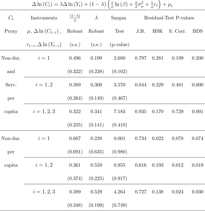
in Table 2. First, we note that (1 )= – the coe¢cient of the aggregate return – is not signi…cant for any instrument list and consumption measure used here. Income growth
becomes signi…cant when we use more than one lag for instruments. When is signi…cant,
estimates range from 0:300 to 0:559, in line with the …ndings of Campbell and Mankiw. Sargan-test results are also line with theirs – the null is never rejected.
6We must stress that we found evidence of heteroskedasticity at the annual frequency. However,
Despite these …ndings, diagnostic-test results show signs of misspeci…cation – except for
one regression. The strongest rejections are for the BDS test, although serial correlation and
ARCH tests are also signi…cant for non-durable consumption. As before, the Jarque and
Bera (1987) test does not reject the null of normal errors.
Even discarding diagnostic-test results, since (1 )= is insigni…cant in all regressions, we are back to Campbell and Mankiw’s basic setup: quadratic utility with rule-of-thumb
applying to consumption and income alone. Here, because of the observational equivalence
result in Section 2.2, we cannot conclude that indeed measures the proportion of
rule-of-thumb agents. It might be an estimate of ck
yk in King, Plosser and Rebelo’s (1988) optimizing
model.
3.4
Non-Linear Models and Rule-of-Thumb Tests
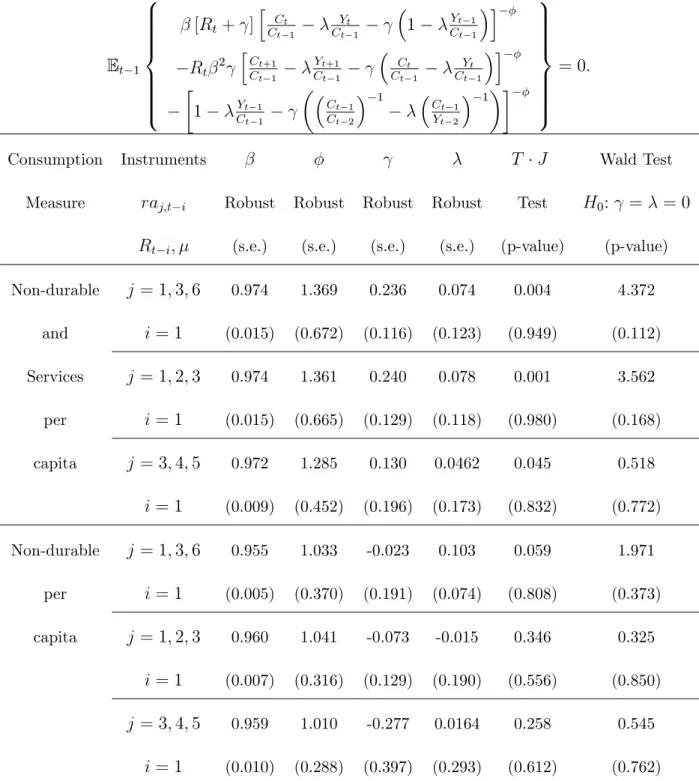
In Table 3, we present results of the general model estimated in Weber (2002), where the
unconstrained agent has external habit and there is rule-of-thumb behavior, i.e., equation
(27). At the5% signi…cance level, we cannot reject H0 : = 0 in any estimated regression. Thus, as in Weber, there is no sign of rule-of-thumb behavior in consumption in the presence
of external habit. However, contrary to Weber’s results, with one exception, we cannot reject
H0 : = 0 in testing at5%, which is evidence that there is no habit formation in preferences. To examine this issue further, we also performed a joint wald test with H0 : ( ; )
0
= (0;0)0
,
which presented overwhelming evidence that the null is true. It is also worth noting that
the intertemporal discount rate is always signi…cant, with estimates ranging from0:955to
ranging from1:010to1:369. Moreover, in all cases, Hansen’s (1982)T J test did not reject the implicit over-identifying restrictions.
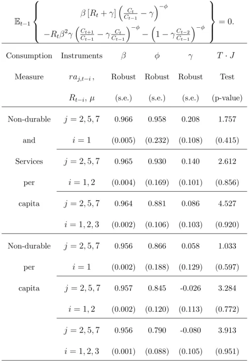
Table 4 shows the results of estimation of equation (28) – the euler equation for the
unconstrained agent with external habit and no rule-of-thumb in aggregating consumption.
Recall that this speci…cation is the preferred one in Weber’s consumption study, who …nds
empirical support for external habit, but not for rule of thumb. Here, however, the habit
formation parameter is insigni…cant for all consumption measures and group of instruments,
while the intertemporal discount rate and the risk aversion coe¢cient are signi…cant
everywhere, ranging from 0:956 to 0:966, and 0:790 to 0:958, respectively. Overall, contrary to Weber’s …ndings, the results in Table 4 show no sign of external habit, since the null that
= 0 is not rejected anywhere in wald tests. As we stressed before, the use of the capital rental rate is critical for the latter result. Here, instead of dispensing with information
contained on the set of all returns, we use this information by aggregating returns into the
capital rental rate as computed by Mulligan (2002). Again, Hansen’s (1982) T J test did
not reject any of the implicit over-identifying restrictions.
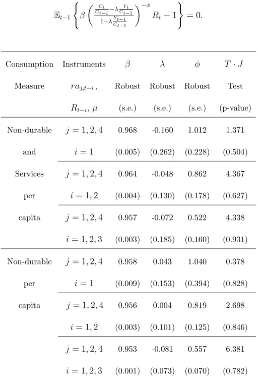
Table 5 considers the estimation of equation (29) – unconstrained agent with CRRA
utility and rule-of-thumb in aggregating consumption. There is no sign of rejection for
Hansen’s T J over-identifying-restriction test. The discount rate and the risk aversion
coe¢cient are both signi…cant everywhere – the …rst ranging from 0:953 to 0:968 and the second from0:522to1:040. The null that = 0is not rejected for any consumption measure and group of instruments. Overall, results from Tables 3 and 5 show no evidence of
rule-of-thumb behavior. This contrasts with evidence presented by Campbell and Mankiw (1989,
The evidence gathered so far suggests that perhaps a reasonable representation for
prefer-ences is an aggregate model with simple CRRA utility without rule-of-thumb in aggregating
consumption. Estimation of this model is reported in Table 6. The discount rate , and the
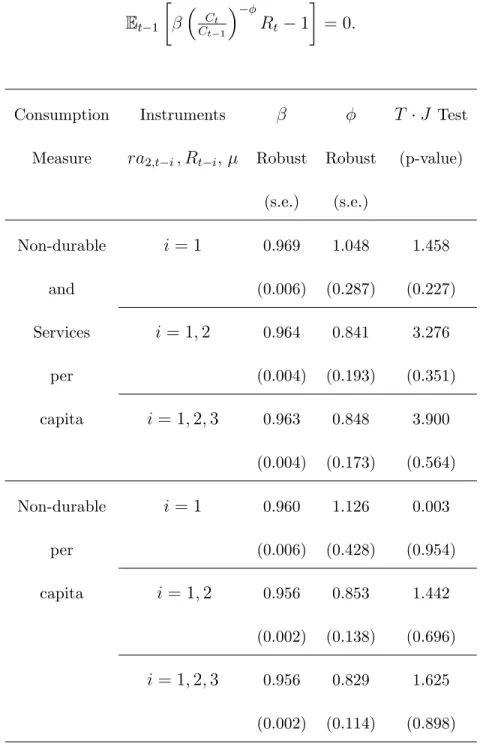
risk aversion coe¢cient are both signi…cant, ranging from 0:956 to 0:969 and form 0:829
to1:126, respectively. There is no single rejection for Hansen’s T J test.
The results in Table 6 for the relative risk-aversion coe¢cient are comparable to those
in Mulligan, although the ones obtained here are robust to inconsistencies arising from
omission of higher-order terms in approximating the euler equation. In terms of empirical
results, robustness in this case is critical. If we truly believe in the linear model, and tested
for the existence of rule-of-thumb as was done in Table 2, we would have concluded for
its existence at the 5% level in four out of six cases. Hence, our best estimates for the importance of rule-of-thumb consumers would range from 0:300 to 0:559, in line with the …ndings of Campbell and Mankiw for the U.S. economy.
4
Conclusions
Our paper has several original contributions to the literature on consumption optimality.
First, we provide a new result on the basic rule-of-thumb regression, showing that it is
obser-vational equivalent to the one obtained in the optimizing model of King, Plosser and Rebelo
(1988). Second, for tests based on the Asset-Pricing Equation, we show that the omission
of the higher-order term in the log-linear approximation yields inconsistent estimates of the
structural parameters when lagged observables are used as instruments. Although Weber
of current rule-of-thumb tests. Third, we show that the nonlinear estimation of a system of
N Asset-Pricing Equations can be done e¢ciently even if the number of asset returns (N)
is high vis-a-vis the number of time-series observations (T), which prevents system estima-tion. We argue that e¢ciency can be restored by aggregating returns into a single measure
that fully captures intertemporal substitution. Indeed, we show that there is no reason why
return aggregation cannot be performed in the nonlinear setting of the Pricing Equation,
since the latter is a linear function of individual returns. Fourth, aggregation of the
non-linear euler equation forms the basis of a new test of rule-of-thumb behavior, which can be
viewed as testing for the importance of rule-of-thumb consumers when the optimizing agent
holds an equally-weighted portfolio of returns or a weighted portfolio of returns. We also
discuss the similarities between the aggregation method proposed here and Mulligan’s (2002)
aggregation leading to the capital rental rate.
Our empirical results are:
1. In Tables 1 and 2, the log-linear tests using an aggregate version of the real return to
wealth – the capital rental rate – show the usual presence of rule-of-thumb behavior in
consumption decisions. However, evidence of the diagnostic tests performed in these
regressions show overwhelming signs of misspeci…cation of the linear model due to
the omission of the higher-order term. This is particularly troublesome since lagged
observables were used as instruments.
2. Non-linear estimation of the aggregate euler equation in Table 3 shows overwhelming
overwhelming signs that = 0 while Table 5 shows overwhelming signs that = 0.
3. In Table 6 we consider a non-linear aggregate model without rule-of-thumb behavior
in consumption and without habit formation. The intertemporal discount factor is
signi…cant and ranges from 0:956 to 0:969 while the relative risk-aversion coe¢cient is precisely estimated ranging from 0:829 to 1:126. There is no evidence of rejection in over-identifying-restriction tests. Taken together, our results show no signs of
ei-ther rule-of-thumb behavior for U.S. consumers or of habit-formation in consumption
decisions once proper econometric tests are performed.
It is important to view our empirical optimality results in perspective. The early
liter-ature on consumption found important puzzles such as excess smoothness (sensitivity), the
equity-premium puzzle, and rule-of-thumb behavior; see Hall (1978), Flavin (1981), Hansen
and Singleton (1982, 1983, 1984), Mehra and Prescott (1985), Campbell (1987), Campbell
and Deaton (1989), Campbell and Mankiw (1989, 1990), and Epstein and Zin (1991). These
studies used time-series methods applied to aggregate consumption data and disaggregate
returns. Later, when panel-data methods were applied to household data and disaggregate
returns, the evidence favored optimal behavior; see Runkle (1991), Attanasio and Browning
(1995), Attanasio and Weber (1995), and Dynan (2000). Some of these panel-data studies
proposed an aggregate-bias explanation for the lack of optimality found in early studies. In
a limited linear setting, the work of Mulligan (2002) on cross-sectional aggregation points
towards the importance of aggregating returns to measure intertemporal substitution in a
representative-agent setting, i.e., with aggregate consumption. Our work shows that
consumption, but linear on returns. The aggregated Pricing Equation is valid regardless of
the number of assets (N) used in estimation and testing, even if N ! 1 at any rate. It is equivalent to the euler equation of an optimizing representative consumer who hold an
equally-weighted or weighted portfolio of traded assets. Therefore, whose return to wealth is
Rt = N1 N
P
i=1
Ri;t orRt= N
P
i=1
!iRi;t, respectively. When the number assets is large, all
idiosyn-cratic noise vanish in these combinations, since Rt = plim N!1
1
N N
P
i=1
Ri;t or Rt = plim N!1
N
P
i=1
!iRi;t.
For that reason, the latter two are closely related to intertemporal substitution measured
with aggregate consumption, a property individual returns seem to lack given the evidence
of early studies. Therefore, the message of this paper is that proper return aggregation is
critical to study intertemporal substitution in a representative-agent framework. This
in-volves aggregating the nonlinear euler equation and performing estimation and testing using
it. In this case, we …nd no evidence of lack of optimality.
References
[1] Abel, A., 1990, “Asset Prices under Habit Formation and Catching Up with the
Jone-ses,“American Economic Review Papers and Proceedings, 80, 38-42.
[2] Araujo, F. and Issler J.V. (2008), “Estimating the stochastic discount factor without a
utility function.” Mimeographed, Graduate School of Economics, Getulio Vargas
Foun-dation.
[3] Attanasio, O., and M. Browning, 1995, “Consumption over the Life Cycle and over the
[4] Attanasio, O., and G. Weber, 1995, “Is Consumption Growth Consistent with
Intertem-poral Optimization? Evidence from the Consumer Expenditure Survey,” Journal of
Political Economy, vol. 103(6), pp. 1121-1157.
[5] Brock,W. A., J. A. Scheinkman, W. D. Dechert and B. LeBaron, 1996. “A test for
independence based on the correlation dimension,” Econometric Reviews, vol. 15(3),
pp. 197-235.
[6] Browning, M., Deaton, A., and Irish, M., 1985, “A Pro…table Approach to Labor Supply
and Commodity Demands over the Life-Cycle,” Econometrica, Volume 53(3), pp.
503-43.
[7] Campbell, J.Y. and Deaton, A. (1989), “Why is Consumption so Smooth?” Review of
Economic Studies, 56:357-374.
[8] Campbell, J.Y., Mankiw, N.G., 1989. “Consumption, income and interest rates:
rein-terpreting the time series evidence.” In: Blanchard, O.J., Fischer, S. (Eds.), NBER
Macroeconomics Annual. MIT Press, Cambridge, MA, pp. 185-214.
[9] Campbell, J.Y., Mankiw, N.G., 1990. “Permanent income, current income, and
con-sumption.” Journal of Business and Economic Statistics, 8, 265-280.
[10] Cushing, M.J. 1992. “Liquidity constraints and aggregate consumption behavior.”
Eco-nomic Inquiry, 30, 134-153.
[11] Deaton, A., 1985. “Panel data from time series of cross-sections,”Journal of
[12] Driscoll, John C. and Aart C. Kraay, 1998, “Consistent Covariance Matrix Estimation
with Spatially Dependent Panel Data,” The Review of Economics and Statistics, Vol.
80, No. 4, pp. 549-560.
[13] Dynan, K., 2000, “Habit Formation in Consumer Preferences: Evidence from Panel
Data,”American Economic Review, vol. 90, pp. 391-406.
[14] Engle, R.F. (1982), “Autoregressive Conditional Heteroskedasticity with Estimates of
the Variance of United Kingdom In‡ation,” Econometrica, 50, pp. 987-1006.
[15] Epstein, L.G., Zin, S.E., 1989. “Substituition, risk aversion and the temporal behavior
of consumption growth and asset returns I: a theoretical framework.” Econometrica,
v.57, p.937-69.
[16] Flavin, M.A., 1981. “The Adjustments of Consumption to Changing Expectations
About Future Income. Journal of Political Economy, 89, 974-1009.
[17] Fuhrer, J.C., Moore, G.R., Schuh, S.D., 1995. “Estimating the linear-quadratic
inven-tory model: maximum likelihood versus generalized methods of moments. Journal of
Monetary Economics, 35, 115-157.
[18] Graham, F.C., 1993. Fiscal policy and aggregate demand: comment. American
Eco-nomic Review,83, 659-666.
[19] Granger, C.W.J., 2008, “A History of Econometrics at the University of California, San
[20] Hall, R.E., 1978. “Stochastic Implications of the Life Cycle-Permanent Income
Hypoth-esis: Theory and Evidence.” Journal of Political Economy, 86, 971-87.
[21] Hall, Robert E. and Frederic S. Mishkin, 1982, “The Sensitivity of Consumption to
Transitory Income: Estimates from Panel Data on Households,”Econometrica, Vol. 50,
No. 2, pp. 461-481.
[22] Hansen, L.P. Singleton, K.J., 1982. “Generalized instrumental variables estimation of
nonlinear rational expectations models. Econometrica, 50, 1269-1286.
[23] Hansen, L.P., Singleton, K.J., 1983. “Stochastic consumption, risk aversion, and the
temporal behavior of asset returns. Journal of Political Economy, 91, 249-265.
[24] Hansen, L.P., Singleton, K.J., 1984. Erratum of the article “Generalized instrumental
variables estimation of nonlinear rational expectations models”. Econometrica, 52 (1),
267-268.
[25] Issler, J. V., Vahid, F., 2001, “Common cycles and the importance of transitory shocks
to macroeconomic aggregates,”Journal of Monetary Economics, vol. 47, 449–475.
[26] Jarque, C.M. and A.K. Bera, 1987, “A Test for Normality of Observations and
Regres-sion Residuals.”International Statistical Review, 55:163-172.
[27] King, R.G., Plosser, C.I. and Rebelo, S.(1988), “Production, Growth and Business
Cycles. II. New Directions,” Journal of Monetary Economics, vol. 21, pp. 309-341.
[28] Mankiw, N.G., 1981. “The permanent income hypothesis and the real interest rate.”
[29] Mao, C. S., 1990. “Hypothesis testing and …nite sample properties of generalized method
of moments estimators: a Monte Carlo study.” Working paper 90-12, Federal Reserve
Bank of Richmond.
[30] Mehra, R., and Prescott, E., 1985, “The Equity Premium: A Puzzle,” Journal of
Mon-etary Economics, 15, 145-161.
[31] Mulligan, C., 2002. “Capital, Interest, and Aggregate Intertemporal Substitution.”
NBER working paper #9373.
[32] Runkle, D. (1991), “Liquidity Constraints and the Permanent Income Hypothesis:
Ev-idence from Panel Data”. Journal of Monetary Economics, 27(1):73-98.
[33] Tauchen, G., 1986. “Statistical properties of generalized method-of-moments estimators
of structural parameters obtained from …nancial market data.”Journal of Business and
Economic Statistics 4, 397-416.
[34] Weber, C.E., 1998. “Consumption spending and the paper-bill spread: theory and
evi-dence.” Economic Inquiry, 36, 575-589.
[35] Weber, C.E., 2002. “Intertemporal non-separability and “rule of thumb” consumption.”
Journal of Monetary Economics, 49, 293-308.
[36] Working, H., 1960. “Note on the correlation of …rst di¤erences of averages in a random
A
Appendix: Tables
Table 1 - Instrumental-Variable Estimation of
ln (Ct) = 1 ln ( ) + 2 2 + 1rt+ t
Ct Instruments 1= Sargan Residual-Test P-values
Proxy ln (Ct i); Robust Test J.B. HSK S. Corr. BDS
rt i; (s.e.) (p-value)
Non-dur. i= 1 0.689 2.337 0.691 0.414 0.129 0.006
and (0.266) (0.126)
Services i= 1;2 0.741 3.086 0.710 0.430 0.129 0.002
per (0.255) (0.379)
capita i= 1;2;3 0.741 3.107 0.710 0.430 0.129 0.002
(0.254) (0.684)
Non-dur. i= 1 0.888 0.002 0.319 0.057 0.214 0.068
per (0.359) (0.966)
capita i= 1;2 0.994 2.425 0.348 0.057 0.227 0.026
(0.342) (0.489)
i= 1;2;3 0.993 2.681 0.348 0.057 0.226 0.026
(0.342) (0.749)
Note: Only 1= reported. Rt is Mulligan’s (2002) after-tax capital rental rate, rt de…ned in
(20). Robust S.E.s use Newey and West (1987). Residual tests report the smallest p-value. J.B.:
Jarque and Bera’s (1987) test. HSK: Heteroskedasticity test: ARCH test with lags 1 and 2. S.
Corr.: LM serial correlation, with lags 1 and 2. BDS: Brock et al.’s (1996) independence test –
Table 2 - Instrumental Variable Estimation of:
ln (Ct) = ln (Yt) + (1 ) 1 ln ( ) + 2 2 + 1rt + t
Ct Instruments (1 ) Sargan Residual-Test P-values
Proxy , ln (Ct i); Robust Robust Test J.B. HSK S. Corr. BDS
rt i; ln (Yt i) (s.e.) (s.e.) (p-value)
Non-dur. i= 1 0.496 0.199 2.680 0.797 0.281 0.199 0.200
and (0.322) (0.238) (0.102)
Serv. i= 1;2 0.389 0.300 3.570 0.844 0.229 0.481 0.000
per (0.264) (0.149) (0.467)
capita i= 1;2;3 0.322 0.341 7.183 0.935 0.170 0.729 0.001
(0.255) (0.141) (0.410)
Non-dur. i= 1 0.667 0.238 0.001 0.734 0.022 0.078 0.074
per (0.691) (0.635) (0.980)
capita i= 1;2 0.361 0.559 0.955 0.616 0.193 0.012 0.019
(0.374) (0.225) (0.917)
i= 1;2;3 0.389 0.529 4.264 0.727 0.138 0.024 0.030
(0.348) (0.199) (0.749)
Table 3 GMM Estimation of Equation (27)
Representative Consumer with Habit Formation and Rule-of-Thumb in Aggregation
Et 1
8 > > > > > > < > > > > > > :
[Rt+ ]
h
Ct
Ct 1
Yt
Ct 1 1
Yt 1 Ct 1
i
Rt 2
hC
t+1 Ct 1
Yt+1 Ct 1
Ct
Ct 1
Yt
Ct 1
i
1 Yt 1 Ct 1
Ct 1 Ct 2
1
Ct 1 Yt 2
1 9 > > > > > > = > > > > > > ; = 0:
Consumption Instruments T J Wald Test
Measure raj;t i Robust Robust Robust Robust Test H0: = = 0
Rt i; (s.e.) (s.e.) (s.e.) (s.e.) (p-value) (p-value)
Non-durable j = 1;3;6 0.974 1.369 0.236 0.074 0.004 4.372
and i= 1 (0.015) (0.672) (0.116) (0.123) (0.949) (0.112)
Services j = 1;2;3 0.974 1.361 0.240 0.078 0.001 3.562
per i= 1 (0.015) (0.665) (0.129) (0.118) (0.980) (0.168)
capita j = 3;4;5 0.972 1.285 0.130 0.0462 0.045 0.518
i= 1 (0.009) (0.452) (0.196) (0.173) (0.832) (0.772)
Non-durable j = 1;3;6 0.955 1.033 -0.023 0.103 0.059 1.971
per i= 1 (0.005) (0.370) (0.191) (0.074) (0.808) (0.373)
capita j = 1;2;3 0.960 1.041 -0.073 -0.015 0.346 0.325
i= 1 (0.007) (0.316) (0.129) (0.190) (0.556) (0.850)
j = 3;4;5 0.959 1.010 -0.277 0.0164 0.258 0.545
i= 1 (0.010) (0.288) (0.397) (0.293) (0.612) (0.762)
Note: Estimated by GMM. Robust S.E. estimates use Newey and West’s (1987) procedure and
Table 4 GMM Estimation of Equation (28)
Representative Consumer with Habit Formation and No Rule-of-Thumb in Aggregation
Et 1
8 > > < > > :
[Rt+ ] CCt
t 1
Rt 2
Ct+1 Ct 1
Ct
Ct 1 1
Ct 2 Ct 1
9 > > = > > ;
= 0:
Consumption Instruments T J
Measure raj;t i; Robust Robust Robust Test
Rt i; (s.e.) (s.e.) (s.e.) (p-value)
Non-durable j = 2;5;7 0.966 0.958 0.208 1.757
and i= 1 (0.005) (0.232) (0.108) (0.415)
Services j = 2;5;7 0.965 0.930 0.140 2.612
per i= 1;2 (0.004) (0.169) (0.101) (0.856)
capita j = 2;5;7 0.964 0.881 0.086 4.527
i= 1;2;3 (0.002) (0.106) (0.103) (0.920)
Non-durable j = 2;5;7 0.956 0.866 0.058 1.033
per i= 1 (0.002) (0.188) (0.129) (0.597)
capita j = 2;5;7 0.957 0.845 -0.026 3.284
i= 1;2 (0.002) (0.120) (0.113) (0.772)
j = 2;5;7 0.956 0.790 -0.080 3.913
i= 1;2;3 (0.001) (0.088) (0.105) (0.951)
Table 5 Instrumental Variable Estimation of Equation (29)
Representative consumer with CRRA Utility and Rule-of-Thumb in Aggregation
Et 1
(
Ct Ct 1
Yt Ct 1
1 CtYt 1
1
Rt 1
) = 0:
Consumption Instruments T J
Measure raj;t i; Robust Robust Robust Test
Rt i; (s.e.) (s.e.) (s.e.) (p-value)
Non-durable j = 1;2;4 0.968 -0.160 1.012 1.371
and i= 1 (0.005) (0.262) (0.228) (0.504)
Services j = 1;2;4 0.964 -0.048 0.862 4.367
per i= 1;2 (0.004) (0.130) (0.178) (0.627)
capita j = 1;2;4 0.957 -0.072 0.522 4.338
i= 1;2;3 (0.003) (0.185) (0.160) (0.931)
Non-durable j = 1;2;4 0.958 0.043 1.040 0.378
per i= 1 (0.009) (0.153) (0.394) (0.828)
capita j = 1;2;4 0.956 0.004 0.819 2.698
i= 1;2 (0.003) (0.101) (0.125) (0.846)
j = 1;2;4 0.953 -0.081 0.557 6.381
i= 1;2;3 (0.001) (0.073) (0.070) (0.782)
Table 6 Instrumental Variable Estimation of General Equation (30)
Representative consumer with CRRA Utility and No Rule-of-Thumb in Aggregation
Et 1 CCtt1 Rt 1 = 0:
Consumption Instruments T J Test
Measure ra2;t i; Rt i; Robust Robust (p-value)
(s.e.) (s.e.)
Non-durable i= 1 0.969 1.048 1.458
and (0.006) (0.287) (0.227)
Services i= 1;2 0.964 0.841 3.276
per (0.004) (0.193) (0.351)
capita i= 1;2;3 0.963 0.848 3.900
(0.004) (0.173) (0.564)
Non-durable i= 1 0.960 1.126 0.003
per (0.006) (0.428) (0.954)
capita i= 1;2 0.956 0.853 1.442
(0.002) (0.138) (0.696)
i= 1;2;3 0.956 0.829 1.625
(0.002) (0.114) (0.898)