Air/sea DMS gas transfer in the North Atlantic: evidence for limited interfacial gas exchange at high wind speed

(1)

ACPD

13, 13285–13322, 2013

Air/sea DMS gas transfer in the North

Atlantic

T. G. Bell et al.

Title Page

Abstract Introduction

Conclusions References

Tables Figures

◭ ◮

Back Close

Full Screen / Esc

Printer-friendly Version Interactive Discussion

Discussion

P

a

per

|

Dis

cussion

P

a

per

|

Discussion

P

a

per

|

Discussio

n

P

a

per

|

Atmos. Chem. Phys. Discuss., 13, 13285–13322, 2013 www.atmos-chem-phys-discuss.net/13/13285/2013/ doi:10.5194/acpd-13-13285-2013

Atmospheric Chemistry and Physics

Open Access

Discussions

Geoscientiic Geoscientiic

This discussion paper is/has been under review for the journal Atmospheric Chemistry and Physics (ACP). Please refer to the corresponding final paper in ACP if available.

Air/sea DMS gas transfer in the North

Atlantic: evidence for limited interfacial

gas exchange at high wind speed

T. G. Bell1,*, W. De Bruyn2, S. D. Miller3, B. Ward4, K. Christensen5, and E. S. Saltzman1

1

Department of Earth System Science, University of California, Irvine, CA, USA

2

Department of Physical Sciences, Chapman University, Orange, California, CA, USA

3

Atmospheric Sciences Research Center, State University of New York at Albany, NY, USA

4

School of Physics, National University of Ireland, Galway, Ireland

5

Norwegian Meteorological Institute, Postboks 43, Blindern, 0313 Oslo, Norway

*

now at: Plymouth Marine Laboratory, Prospect Place, The Hoe, Plymouth, PL1 3DH, UK

Received: 29 March 2013 – Accepted: 3 May 2013 – Published: 21 May 2013

Correspondence to: T. G. Bell (tbe@pml.ac.uk)

Published by Copernicus Publications on behalf of the European Geosciences Union.

(2)

ACPD

13, 13285–13322, 2013

Atlantic

T. G. Bell et al.

Title Page

Tables Figures

◭ ◮

Back Close

Full Screen / Esc

Discussion

P

a

per

|

Dis

cussion

P

a

per

|

Discussion

P

a

per

|

Discussio

n

P

a

per

Abstract

Shipboard measurements of eddy covariance DMS air/sea fluxes and seawater con-centration were carried out in the North Atlantic bloom region in June/July 2011. Gas transfer coe_fficients (k660) show a linear dependence on mean horizontal wind speed at

wind speeds up to 11 m s−1. At higher wind speeds the relationship betweenk660 and

5

wind speed weakens. At high winds, measured DMS fluxes were lower than predicted based on the linear relationship between wind speed and interfacial stress extrapolated from low to intermediate wind speeds. In contrast, the transfer coefficient for sensible heat did not exhibit this effect. The apparent suppression of air/sea gas flux at higher wind speeds appears to be related to sea state, as determined from shipboard wave

10

measurements. These observations are consistent with the idea that long waves sup-press near surface water side turbulence, and decrease interfacial gas transfer. This e_ffect may be more easily observed for DMS than for less soluble gases, such as CO₂, because the air/sea exchange of DMS is controlled by interfacial rather than bubble-mediated gas transfer under high wind speed conditions.

15

1 Introduction

Gas exchange between the ocean and atmosphere is a major term in the global bud-gets of many compounds with biogeochemical and climatic importance. For example, air/sea gas exchange controls the oceanic uptake and/or release of carbon dioxide, oxygen, nitrous oxide, methane, halocarbons, dimethylsulfide (DMS) and ammonia and

20

the cycling of volatile toxic pollutants such as mercury and many pesticides (Butler et al., 2010; Stramma et al., 2008; Bange et al., 2009; Lana et al., 2011; Johnson et al., 2008; Sabine et al., 2004; Soerensen et al., 2010; Harman-Fetcho et al., 2000). Parameterization of air/sea gas transfer is one of the major uncertainties in global bio-geochemical models (e.g. Elliott, 2009). A better understanding of gas transfer rates

(3)

ACPD

13, 13285–13322, 2013

Atlantic

T. G. Bell et al.

Title Page

Tables Figures

◭ ◮

Back Close

Full Screen / Esc

Discussion

P

a

per

|

Dis

cussion

P

a

per

|

Discussion

P

a

per

|

Discussio

n

P

a

per

|

and their controlling factors is needed in order to predict how air/sea gas fluxes will vary in the future in response to changing climate and anthropogenic emissions.

The air/sea flux of gas is proportional to the concentration difference across the interface (∆C) and a gas transfer coefficient,K, expressed in water-side units:Kw(Liss

and Slater, 1974):

5

FDMS=Kw·∆C (1)

Kw includes the combined effect of diffusive and turbulent processes on both sides of

the interface that limit the transfer of gas between the bulk seawater and air phases. The physical forcing for gas transfer is wind stress and buoyancy at the sea surface. Whitecaps/bubble production, wind/wave interactions and surface films all play a role

10

in determining the rate of gas transfer (Wanninkhof et al., 2009).

Estimates of oceanic gas transfer coefficients and their dependence on wind speed, diffusivity, and solubility have been derived from the global oceanic inventory of excess radiocarbon, laboratory wind–wave experiments, and dual tracer experiments with3He and SF6(e.g. Ocampo-Torres et al., 1994; Watson et al., 1991; Sweeney et al., 2007;

15

Liss and Merlivat, 1986; Wanninkhof, 1992; Wanninkhof and McGillis, 1999; Nightin-gale et al., 2000; Ho et al., 2006; Broecker et al., 1985; Wanninkhof et al., 2009). A number of physical process-based models have been developed to estimate air/sea gas transfer rates. These include the effects of turbulent transport, buoyancy, bubbles, Langmuir circulation and wind/wave interactions (e.g. Fairall et al., 1996, 2011; Hare

20

et al., 2004; Johnson, 2010; Rutgersson et al., 2011; Soloviev et al., 2007; Soloviev, 2007).

Gas solubility exerts a significant influence on air/sea exchange. Gas transfer rates are controlled by transport on the seawater side of the interface for relatively insoluble gases like CO2. More soluble gases, like acetone, are controlled primarily by transport

25

on the atmospheric side of the interface. Solubility also determines the extent to which whitecaps and bubbles contribute to gas transfer (Woolf, 1997). For example, bubbles

(4)

ACPD

13, 13285–13322, 2013

Atlantic

T. G. Bell et al.

Title Page

Tables Figures

◭ ◮

Back Close

Full Screen / Esc

Discussion

P

a

per

|

Dis

cussion

P

a

per

|

Discussion

P

a

per

|

Discussio

n

P

a

per

are believed to dominate the gas transfer for CO₂ at high wind speeds, while they are a relatively minor component of the flux for DMS.

The influence of wind/wave interactions on gas transfer is an understudied aspect of air/sea gas exchange. There is evidence that the presence of swell may modify the roughness of wind-seas (García-Nava et al., 2012, 2009). Laboratory studies have

5

demonstrated that flow separation at wave crests can create a shielding effect on the lee side of the wave, and reduce the friction velocity at the surface (Veron et al., 2007; Reul et al., 1999, 2008). Some models have attempted to incorporate this effect into the estimate of gas transfer (Soloviev et al., 2007; Soloviev, 2007; Soloviev and Schlussel, 1994), but it has not been observed directly in the field (Nightingale et al., 2000; Smith

10

et al., 2011).

Micrometeorological techniques involve the direct determination of air/sea gas fluxes on the atmospheric side of the interface. Eddy covariance measurements have been made at sea for CO₂ (e.g. McGillis et al., 2001, 2004; Miller et al., 2010) and for DMS (Huebert et al., 2004, 2010; Marandino et al., 2007, 2008, 2009; Blomquist et al., 2006;

15

Yang et al., 2011). Micrometeorological techniques have the potential to measure gas transfer rates on shorter time scales than the integrative geochemical or surface ocean budget techniques, providing the opportunity to study the response of the sea surface to local changes in wind and wave fields. The difference in solubility between DMS and CO₂ o_ffers the potential to di_fferentiate between interfacial and bubble-mediated gas

20

transfer (Blomquist et al., 2006).

This paper presents eddy covariance measurements of air/sea DMS flux on a June/July 2011 cruise aboard the R/V Knorr in the North Atlantic Ocean (Knorr_11). The cruise started and ended at Woods Hole, Massachusetts, USA (41.53◦N, 70.68◦W; Fig. 1) and roughly half of the cruise was spent in the high productivity,

25

high latitude waters of the North Atlantic bloom. This study was designed to increase the observational data base for gas transfer in a region of the oceans where biologi-cal activity results in exceptionally large air/sea DMS and CO2fluxes. This study also

(5)

anoma-ACPD

13, 13285–13322, 2013

Atlantic

T. G. Bell et al.

Title Page

Tables Figures

◭ ◮

Back Close

Full Screen / Esc

Discussion

P

a

per

|

Dis

cussion

P

a

per

|

Discussion

P

a

per

|

Discussio

n

P

a

per

|

lously high DMS gas transfer coefficients inconsistent with current models (Marandino et al., 2008).

2 Methods

2.1 Mast-mounted instrumentation and data acquisition setup

The eddy covariance setup was mounted on the Knorr bow mast at a height of 13.6 m

5

above the sea surface. This included two sonic anemometers (Campbell CSAT3), mea-suring 3-dimensional winds and sonic temperature and two Systron Donner Motion Pak II (MPII) units measuring platform angular rates and accelerations. Air sampling inlets for DMS, consisting of 3/8′′ ID Teflon tubes, were mounted 0.2 m from the sensing region of the anemometers at the same height. Analog signals from the

anemome-10

ters, motion sensors, and mass spectrometer were filtered using Butterworth filters (15 Hz cutoff frequency) and logged at 50 Hz using a multichannel data acquisition system (National Instruments SCXI-1143) and custom Labview™ software. Data from the ship’s compass and GPS systems were logged digitally at 1 Hz.

2.2 Atmospheric DMS

15

Atmospheric DMS levels were measured using an atmospheric pressure chemical ion-ization mass spectrometer (API-CIMS). DMS detection involved proton transfer from H₃O+ to DMS in the gas phase, followed by quadrupole mass filtering and ion counting detection of protonated DMS (Marandino et al., 2007; Blomquist et al., 2010; Bandy et al., 2002). A new instrument was used in this study (UCI mesoCIMS), consisting of

20

a heated ion source (400◦C, operated at 550 Torr), a declustering region (0.5 Torr), and differentially-pumped quadrupole entry and ion detection chambers. A full description of the instrument is provided in the Supplement.

The mesoCIMS was located in a container van on the Knorr 02 deck, one level above the main deck. Air was drawn from the bow mast inlet to the instrument van through

25

(6)

ACPD

13, 13285–13322, 2013

Atlantic

T. G. Bell et al.

Title Page

Tables Figures

◭ ◮

Back Close

Full Screen / Esc

Discussion

P

a

per

|

Dis

cussion

P

a

per

|

Discussion

P

a

per

|

Discussio

n

P

a

per

a 28 m length of 3/8′′ ID Teflon tubing at a flow rate of 80 L min−1. These conditions provided fully turbulent flow (Re>10 000). The air flow rate was maintained by a rotary vane pump, with active control provided by a mass flow meter, automated butterfly valve, and PID controller. An air flow of 1 L min−1 was drawn off the main inlet flow through a Nafion™ membrane drier and through the mass spectrometer ion source.

5

This air flow was controlled by a mass flow controller and diaphragm pump.

Standardization of DMS measurements was accomplished by introducing a tri-deuterated DMS gas standard (d3-DMS) into the main air flow a few cm downstream of the air intake. The preparation and delivery of DMS gas standards is described in the Supplement. Protonated DMS (m/z=63) and d3-DMS (m/z=66) were continuously

10

monitored in selected ion mode with a 45 ms dwell time and a delay of 5 ms. The sen-sitivity of the instrument to DMS during the cruise was approximately 100 Hz ppt−1, as estimated from the response to the d3-DMS standards. Every two hours, a 3-way valve mounted on the bow mast diverted the flow of gas standard to waste. The response of the d3-DMS signal to this event provides a measure of the delay and frequency

15

response loss associated with the inlet tubing.

Atmospheric DMS levels were calculated as follows:

DMSa=

S63

S66

· FStd FTotal

·CTank (2)

WhereS63 andS66 represent blank-corrected signals from DMS and d3-DMS

respec-tively (Hz),FStdandFTotalare the gas flow rates of the d3-DMS standard and the inlet air

20

(L min−1), and CTank is the gas standard mixing ratio. The raw d3-DMS signal was

av-eraged over each 10 min flux interval to remove variability caused by motion sensitivity of the mass flow controller used to supply the gas standard on this cruise.

2.3 Seawater DMS

DMS in seawater was continuously monitored using a second API-CIMS instrument

25

(7)

ACPD

13, 13285–13322, 2013

Atlantic

T. G. Bell et al.

Title Page

Tables Figures

◭ ◮

Back Close

Full Screen / Esc

Discussion

P

a

per

|

Dis

cussion

P

a

per

|

Discussion

P

a

per

|

Discussio

n

P

a

per

|

and performance of the mass spectrometer and equilibrator are given in Saltzman et al. (2009) and are only briefly described here. The miniCIMS ion source chem-istry and principles of detection are similar to those described earlier. This instrument uses quadrupole and ion detection electronics from a modified residual gas analyzer (Stanford Research Systems RGA-200). It is less sensitive than the mesoCIMS, but

5

adequate to detect DMS over the range of concentrations encountered in the surface of the open ocean.

The equilibrator construction consists of a coiled outer PFA tube (8 m×3/8′′ID) and a porous inner concentric PTFE membrane inner tube (3 mm ID, 60–70 % porosity; International Polymer Engineering). Surface seawater was supplied by the ship’s

non-10

toxic bow pumping system, with an intake depth of 6 m. A seawater flow of approxi-mately 1 L min−1was supplied to the equilibrator. The seawater flow rate was monitored using a GEMS flow meter (Gems Sensors & Controls; P/N 155421). A purified air coun-terflow of 400 mL min−1flowed through the inner membrane tube (Aadco Instruments Pure Air Generator). The air exiting the equilibrator was diluted with purified air to give

15

a total flow of 1.5 L min−1, passed through a Nafion membrane drier (Perma Pure MD-110-72FP) and directed through the ion source. The ion source in this instrument was operated at 1 atmosphere. All gas flows were mass flow controlled and logged. In high wind conditions, a de-bubbling reservoir was inserted in the seawater flow and a peri-staltic pump was used to deliver bubble-free seawater to the equilibrator. The quantity

20

of air in the seawater line was never sufficient to significantly bias seawater DMS levels. The seawater measurements were calibrated by continuously adding isotopically-labeled aqueous d3-DMS standard to the seawater flow prior to entering the equilibra-tor. A working standard of 0.13 mM d3-DMS was delivered at a flow rate of 30 µl min−1 using a syringe pump (New-Era NE300). The working standard was prepared daily by

25

dilution of a primary standard (43 mM d3-DMS in ethanol, prepared prior to the cruise) with deionized water.

(8)

ACPD

13, 13285–13322, 2013

Atlantic

T. G. Bell et al.

Title Page

Tables Figures

◭ ◮

Back Close

Full Screen / Esc

Discussion

P

a

per

|

Dis

cussion

P

a

per

|

Discussion

P

a

per

|

Discussio

n

P

a

per

The DMS concentration in seawater in the equilibrator is calculated as follows:

DMSSW=

S63

S66

· FStd FSW

·CStd (3)

S63 and S66 represent the average blank-corrected ion currents (pA) of protonated

DMS (m/z=63) and d3-DMS (m/z=66), respectively, CStd is the concentration of

d3-DMS liquid standard (nM), FStd is the syringe pump flow rate (L min− 1

), and FSW

5

is the seawater flow rate (L min−1). Seawater concentrations were averaged at 5 min intervals.

Prior deployments of the miniCIMS utilized a gas standard added to the air stream as it exited the equilibrator (Saltzman et al., 2009). This approach requires complete equilibration across the membrane, which requires some effort to quantitatively

vali-10

date during cruise conditions. The use of liquid standards was prompted by concern regarding the possible loss of gas exchange e_fficiency of the equilibrator membrane due to fouling by gelatinous material encountered during passage through phytoplank-ton blooms. Although apparently rare, this effect was observed during a recent cruise in the South Pacific (S. J. Royer, personal communication, 2011). In that case, the

15

membrane was completely blocked and required cleaning with strong acid to restore gas exchange. The use of a liquid standard eliminates the requirement for complete equilibration, since both the natural DMS and the d3-DMS standard are transported across the membrane.

Underway lines can become contaminated with algal/bacterial mats, which can alter

20

the concentrations of various biogeochemically produced compounds (Juranek et al., 2010). To address this issue we periodically placed an underwater pump over the side of the ship and made near-surface measurements. DMS concentrations from the un-derwater pump at 5 m (Fig. 2c, pink squares) compared well with those from the ves-sel’s non-toxic supply (Fig. 2c, green circles). These comparisons show that the ship’s

25

(9)

ACPD

13, 13285–13322, 2013

Atlantic

T. G. Bell et al.

Title Page

Tables Figures

◭ ◮

Back Close

Full Screen / Esc

Discussion

P

a

per

|

Dis

cussion

P

a

per

|

Discussion

P

a

per

|

Discussio

n

P

a

per

|

2.4 DMS flux calculation (eddy covariance data processing and quality control)

The calculation of DMS air/sea flux from the shipboard measurements involved the following steps: (1) correction of the measured apparent winds for ship orientation and motion; (2) adjustment of the relative timing of wind and DMS measurements to correct for delay in the inlet tubing; (3) computation of the DMS flux,< w′c′>; (4) identification

5

of intervals with excessive flux at low frequency; and (5) correction for flux loss due to attenuation of high frequency fluctuations in the inlet tubing. Momentum and heat fluxes were also computed.

The measured winds were corrected for ship motion using 3-dimensional acceler-ations and angular rates from the MotionPak II, GPS and compass. The measured

10

winds are rotated into the ship frame of reference, resulting in zero mean vertical wind and a single horizontal wind vector. These relative winds are then transformed into an Earth frame of reference. Details of the motion correction procedure are given by Edson et al. (1998) and Miller et al. (2008).

The 28 m inlet tubing introduced a delay of about 2.2 s between the wind signal

15

and the DMS signal. This delay was estimated by periodically cycling the 3-way valve delivering d3-DMS to the inlet and recording the time delay between the voltage driving the valve and the resulting change in DMS signal. A similar estimate of the delay was obtained by optimizing the cross correlation between DMS and vertical wind. DMS fluxes were calculated for 10 min flux intervals by integrating the frequency-weighted

20

cospectral density of DMS and vertical wind. No corrections were made for fluctuations in air density due to changes in water vapor or temperature (i.e. Webb et al., 1980) because the air stream was dried, passed through a considerable length of tubing, and heated prior to analysis (Marandino et al., 2007). The internal d3-DMS standard exhibited negligible covariance with vertical wind, confirming that no density correction

25

is required.

Flux intervals exhibiting excessive flux (either positive or negative) at low frequen-cies were flagged and eliminated from the data set. These can result from changing

(10)

ACPD

13, 13285–13322, 2013

Atlantic

T. G. Bell et al.

Title Page

Tables Figures

◭ ◮

Back Close

Full Screen / Esc

Discussion

P

a

per

|

Dis

cussion

P

a

per

|

Discussion

P

a

per

|

Discussio

n

P

a

per

environmental conditions, such as the passage of atmospheric fronts, changes in wind direction, transects across oceanographic fronts, etc. and presumably do not reflect the local air/sea flux. These intervals were identified by examining the cumulative sum (low to high frequency) of normalized flux (Fsum/FDMS) as a function offnorm(f.z/U10n),

wheref is frequency (Hz),z is the measurement height, andU10nis mean wind speed 5

at 10 m height and for neutral conditions. The criteria for elimination are outlined in the Supplemental Material. This process removed 461 of the 1437 flux intervals. This treatment resulted in reduced scatter in the data but did not introduce an obvious bias. The distortion of air flow over the research vessel is a source of uncertainty in eddy covariance measurements. Flow distortion is believed to have a relatively small effect

10

on scalar fluxes (Pedreros et al., 2003). To minimize the impact of flow distortion, ship-board eddy covariance studies typically use relative wind sector as a quality control criterion. Following careful analysis of Knorr_11 wind sector data (see Supplement) flux intervals with a mean relative wind direction>±90◦ were excluded.

Diffusion of DMS during passage through the inlet tubing caused attenuation of

fluc-15

tuations in the mixing ratio at the detector relative to those in ambient air (Massman, 2000; Lenschow and Raupach, 1991). This e_ffect is quite small at the high air flow rates used in this study. The process was modeled as a low pass first-order Butterworth fil-ter, with a time constant adjusted to match the response of the DMS signal to a step change in d3-DMS at the inlet induced by switching the 3-way valve. This filter was

20

applied in an inverse mode to the DMS signal. Flux- and frequency-normalized DMS cospectra were bin averaged into 2 m s−1 wind speed bins. Binned cospectra were inverse-filtered to give an estimate of the high frequency flux signal lost in the tubing. A “gain” (Ghf) was then computed from the ratio of these fluxes.Ghfwas computed for flux

frequencies<1 Hz to avoid the amplification of noise (Blomquist et al., 2010).Ghf

dis-25

played a small linear dependence on mean wind speed (Ghf=1.0079+0.0008.U10n).

(11)

ACPD

13, 13285–13322, 2013

Atlantic

T. G. Bell et al.

Title Page

Tables Figures

◭ ◮

Back Close

Full Screen / Esc

Discussion

P

a

per

|

Dis

cussion

P

a

per

|

Discussion

P

a

per

|

Discussio

n

P

a

per

|

2.5 DMS gas transfer velocity calculation

Total gas transfer velocities were calculated from the cruise data using the equation:

KDMS=

FDMS

∆C =

FDMS

DMSsw−DMSair·HDMS

(4)

WhereF_DMS is the measured DMS air/sea flux (mol m−2s−1), DMS_sw is the seawater DMS level (mol m−3), DMSairis the atmospheric DMS partial pressure (atm), andHDMS

5

is the temperature-dependent DMS solubility in seawater (mol atm−1m−3; Dacey et al., 1984). KDMS values were calculated from the cruise data using 10 min averages of

DMSair, DMSsw, andHDMS, and the 10 min flux calculations described above.

The total gas transfer velocity of DMS (KDMS) reflects the combined effect of

pro-cesses at both the air and water sides of the air/sea interface. The relative

impor-10

tance of air vs. water side resistance varies as a function of wind speed and solubility (McGillis et al., 2000). Our Knorr_11 cruise observations were used in conjunction with the NOAA COARE gas transfer model (version 3.1v) to estimate the air side gas trans-fer coefficient for DMS associated with each of the air/sea flux measurements (Fairall et al., 2011). The water side only gas transfer coefficient,kw, was then obtained from

15

the expression:

kw=

1

K_DMS−

1

α·k_a −1

(5)

whereK_DMSis the total DMS gas transfer coefficient,α is the dimensionless Henry’s Law constant for DMS, and ka is the air side gas transfer coefficient obtained from

NOAA COARE. The average (mean) difference between kw and KDMS was 6 %. To

20

facilitate comparison of these results with various gas transfer parameterizations, kw

was normalized to a Schmidt number of 660 (CO₂at 25◦C):

k660=kw·

660

ScDMS

−1₂

(6)

(12)

ACPD

13, 13285–13322, 2013

Atlantic

T. G. Bell et al.

Title Page

Tables Figures

◭ ◮

Back Close

Full Screen / Esc

Discussion

P

a

per

|

Dis

cussion

P

a

per

|

Discussion

P

a

per

|

Discussio

n

P

a

per

whereSc_DMSis calculated according to Saltzman et al. (1993) using the in situ seawa-ter temperature recorded at the bow of the ship.

2.6 Surface wave measurements

Wave measurements were conducted using a 75 kHz ultrasonic sensor (U-GAGE QT50U, Banner Engineering) in combination with a ±20 ms−2 two-axis linear

ac-5

celerometer (DE-ACCM2G2, Dimension Engineering). The ultrasonic sensor was mounted at the end of a steel pole, which was suspended vertically through the hawse-hole at the bow of the ship, and then bolted to a mount that had been welded to the ship. The accelerometers were attached to the top of the steel pole, and were aligned to measure pitch and roll. Analog outputs of the ultrasonic sensor and accelerometer

10

were logged at 100 Hz.

The ultrasonic sensor was programmed for a range of 8 m and an update rate of 10 Hz. Ultrasound pulses were emitted and the time lag of the echo recorded. The dis-tance to the undulating surface was determined using the speed of sound with compen-sation for changes in air temperature. Ship motion was removed using the acceleration

15

data, and the residual signal represents a time series of sea surface elevation. These data were bandpass-filtered between 0.05 and 0.5 Hz. One-dimensional surface wave spectra were produced in 30 min averages. This method was compared to data from a commercially-available waverider (Datawell Directional Waverider Mk III) during an experiment in Norway, and yielded good agreement (Christensen et al., 2012). For the

20

dataset here, a comparison was made with the output from the ECMWF Wave Model (WAM), which 6 hourly output and 0.1◦horizontal resolution. The shipboard wave sen-sor data contains more variability (more consistent with changes in measured local winds), but on average agrees well (within 10 %) with WAM with respect to significant wave height and mean and peak periods.

(13)

ACPD

13, 13285–13322, 2013

Atlantic

T. G. Bell et al.

Title Page

Tables Figures

◭ ◮

Back Close

Full Screen / Esc

Discussion

P

a

per

|

Dis

cussion

P

a

per

|

Discussion

P

a

per

|

Discussio

n

P

a

per

|

2.7 Whitecaps

Whitecap areal coverage was measured using a digital camera (CC5MPX, Campbell Scientific) trained on the sea surface to collect images at a sample period of about 1 s. The camera is housed in an enclosure with a fan/heater to control condensation. Images were post-processed to calculate the whitecap fraction of the sea surface,

fol-5

lowing Callaghan and White (2009).

3 Results

3.1 Cruise track, meteorological, and oceanographic setting

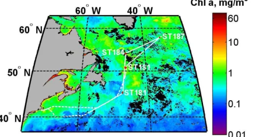
The cruise track for this study was north from Woods Hole, MA through the Gulf Stream and Northwest Atlantic shelf into the high latitude North Atlantic (Fig. 1). The ship

re-10

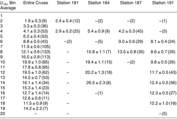
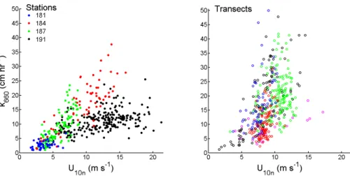
turned to Woods Hole via North Atlantic Drift and Northwest Atlantic Shelf waters. The cruise was carried out in early–mid summer from 24 June–18 July 2011 (DOY 175– 199). The majority of the sampling time was spent north of 50◦N in the Arctic biogeo-chemical province as defined by Longhurst (1995). Four stations in this region (ST181, ST184, ST187, ST191) were occupied for periods of 24 h or more and the remainder of

15

the data was collected underway (Fig. 1, shaded gray in Fig. 2). Station locations were selected to sample regions of elevated seawater DMS and pCO2 drawdown and/or

were defined opportunistically so as to collect data during strong frontal events with intermediate to high wind speeds.

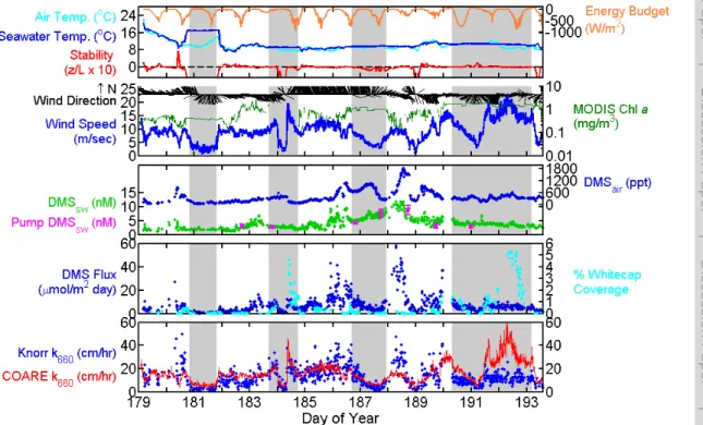
Meteorological and oceanographic measurements during the cruise are shown as

20

time series in Fig. 2. Sea surface temperatures (SST) ranged from roughly 15◦C in the Gulf Stream region to about 10◦C in the high latitude North Atlantic. Surface air temperatures were within±1–2◦C of SST for most of the cruise, with the exception of the Gulf Stream, where SST was several degrees warmer than the overlying air. Bulk sensible heat fluxes typically ranged from−20 to +40 W m−2. Atmospheric boundary

25

(14)

ACPD

13, 13285–13322, 2013

Atlantic

T. G. Bell et al.

Title Page

Tables Figures

◭ ◮

Back Close

Full Screen / Esc

Discussion

P

a

per

|

Dis

cussion

P

a

per

|

Discussion

P

a

per

|

Discussio

n

P

a

per

layer stability was close to neutral (defined as |z/L|<0.07) for >75 % of the cruise. The atmosphere was consistently unstable (z/L<−0.07) in the Gulf Stream (DOY 181) and during the low wind speed period on DOY 184. A stable atmosphere suppresses the size of turbulent eddies, which Yang et al. (2011) identify as potentially anoma-lous in their eddy covariance data. The Knorr_11 cruise encountered z/L>0.05 very

5

infrequently (<8 % of the cruise) and with no apparent bias upon the data.

The cruise track involved transit across strong gradients in chlorophyll associated with the continental shelf and the highly productive North Atlantic bloom region (Fig. 1). Chlorophyllaconcentrations along the ship track were extracted from 4 km resolution MODIS AQUA satellite ocean color images. These data ranged from 0.2–1.9 mg m−3

10

(Fig. 2b). A high chlorophyll region was encountered over the relatively shallow Grand Banks coastal shelf on the northward transect (DOY 180). Numerous phytoplankton blooms were encountered in the high latitude North Atlantic. Discrete pigment sam-ples collected in these blooms during DOY 187.8–191.0 indicate a mixture of prymne-siophytes (likely coccolithophores), diatoms and dinoflagellates (D. Repeta, personal

15

communication, 2012).

Seawater DMS levels (DMSsw) ranged from about 2 nM in the Gulf Stream to a high

of 10.0–14.3 nM in a large algal bloom West of ST187 (DOY 188). In general, elevated DMS levels in the high latitude North Atlantic are associated with high chlorophyll lev-els. However, the relationship is not simple because DMS production and consumption

20

pathways change due to shifts in species composition and the activities of algal and bacterial populations (Stefels et al., 2007). A previous cruise in this region found high DMS_sw levels in conjunction with the MODIS measurement of particulate inorganic carbon (Marandino et al., 2008) and a similar correspondence was observed during Knorr_11. Atmospheric DMS levels (DMSair) ranged from 64–1867 ppt. In general,

25

higher atmospheric DMS levels were encountered over the highly productive high lat-itude waters. However, DMSair is also influenced by a number of other parameters,

(15)

ACPD

13, 13285–13322, 2013

Atlantic

T. G. Bell et al.

Title Page

Tables Figures

◭ ◮

Back Close

Full Screen / Esc

Discussion

P

a

per

|

Dis

cussion

P

a

per

|

Discussion

P

a

per

|

Discussio

n

P

a

per

|

and atmospheric DMS levels were more than an order of magnitude lower than those in surface seawater. Thus, the air/sea DMS concentration difference was essentially controlled by the DMSsw concentration.

Eddy covariance DMS flux (FDMS) measurements for 10 min flux intervals are shown

in Fig. 2d. DMS flux exhibits a higher degree of variability than either DMSsw or wind

5

speed alone, as expected given that both parameters contribute to control the flux. The lowestF_DMS were observed in the Gulf Stream on DOY 181 with low wind speed and DMSsw, and the highest FDMS were observed during the period of high DMSsw and

wind speed on DOY 188. Gas transfer coefficients were computed from the measured

F_DMS and air/sea concentration difference (Eqs. 4–6) and are shown as a time series

10

in Fig. 2e. In general, variations in the gas transfer coe_fficient correlate with the mean horizontal wind speed (Spearman’s ρ=0.53, α <0.01, n=1083). This correlation is particularly clear during frontal passages when wind speed changed rapidly, such as the end of DOY 181 and during DOY 184. There is a notable exception near the end of the cruise, where gas transfer coefficients hardly varied during a period when wind

15

speeds ranged from 5 to 18 m s−1(DOY 190.1–193.3, ST191).

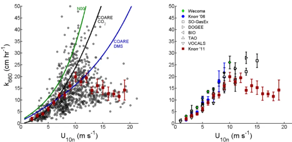
3.2 Gas exchange (k₆₆₀_{) vs. wind speed (}U₁₀_n)

The relationship between k660 and horizontal wind speed is shown as a scatter plot

(Fig. 3a). There is a positive correlation for the data set as a whole, but it is clear that the data are not normally distributed about a single linear trend line. The gas

trans-20

fer coe_fficients exhibit the highest values at intermediate wind speeds (5–10 m s−1), while at higher wind speeds (10–17 m s−1) the gas transfer coefficients level offor even decrease. This is clearly illustrated when the data set is bin-averaged by wind speed (Fig. 3b). Bin averaged gas transfer velocities at wind speeds greater than 11 m s−1 demonstrate a marked departure from the trend observed at lower wind speeds.

25

Bin-averaged Knorr_11 gas transfer coefficients are compared to previously pub-lished shipboard DMS eddy covariance measurements (Fig. 3b). Bin-averaged Knorr_11 gas transfer coefficients are similar to those from previous studies for wind

(16)

ACPD

13, 13285–13322, 2013

Atlantic

T. G. Bell et al.

Title Page

Tables Figures

◭ ◮

Back Close

Full Screen / Esc

Discussion

P

a

per

|

Dis

cussion

P

a

per

|

Discussion

P

a

per

|

Discussio

n

P

a

per

speeds from 0–11 m s−1. Only two previous studies have reported DMS flux data for winds speeds greater than 11 m s−1: the DOGEE and Southern Ocean GasEx studies (Huebert et al., 2010). The Knorr_11 data are significantly lower than the DOGEE and southern Ocean GasEx studies at high wind speeds.

Direct comparison of gas transfer coefficients measured under different conditions

5

in various field programs is complicated by the influence of sea surface temperature (Huebert et al., 2010; Yang et al., 2011). Sea surface temperature influences DMS solubility, which affects the relative importance of air-side vs. water-side resistance. A second issue is the e_ffect of temperature on gas di_ffusivity, which is described by the Schmidt number (ScDMS). The effect of temperature on solubility and ScDMS are

10

accounted for in the calculation ofkw and k660 respectively (see Sect. 2). In addition,

the bubble-driven component of gas transfer (kb) is inversely related to gas solubility

(Woolf, 1997). The temperature effect onkbis difficult to estimate, because it requires

a priori knowledge about the relative contributions of bubble- and non-bubble fluxes under field conditions. Yang et al. (2011) used the COARE model to demonstrate that

15

the uncertainty introduced by this correction is small for DMS (<5 % atU10n=10 m s−1

for a temperature range of 5–27.2◦C). Thekbsolubility adjustment has been applied to

all eddy covariance datasets presented in Fig. 3b with the exception of this study and data from the tropical and sub-tropical Pacific (Marandino et al., 2007, 2009).

The wide spread of gas transfer coefficients and complexity of thekvs.U relationship

20

argues that factors other than wind speed exert a significant control on gas transfer. In an effort to identify these factors, we subdivided the cruise data into segments: each of the four stations and the transects between them (Fig. 4a, b; Table 1). This reveals some significant differences in gas transfer over the course of the cruise. Most notably, ST184 and ST187 define a trend line with a slope (k/U) roughly twice that defined

25

by the data from ST181 and ST191. As mentioned above, at ST191 the gas transfer coefficient shows evidence of leveling offor decreasing with increasing wind speed.

(17)

ACPD

13, 13285–13322, 2013

Atlantic

T. G. Bell et al.

Title Page

Tables Figures

◭ ◮

Back Close

Full Screen / Esc

Discussion

P

a

per

|

Dis

cussion

P

a

per

|

Discussion

P

a

per

|

Discussio

n

P

a

per

|

a similar lowerk/U bound as the station data, but a considerably wider range. Taken alone, the transect measurements give the impression of very steep wind speed de-pendence. More likely, the wide range ofk/U reflects the much larger variability in con-ditions (DMS_sw, wind speed, waves) encountered during transects. To our knowledge, there are no previous eddy covariance gas flux studies comparing data from station

5

and transect measurements.

An earlier cruise in the high latitude North Atlantic coccolithophore bloom southwest of Iceland reported DMS gas transfer velocities that were substantially elevated relative to typical open ocean data (Knorr_07, Marandino et al., 2008). Marandino et al. (2008) speculated that the anomaly was caused by accumulation of DMS- or DMSP-rich

bio-10

logical material at the sea surface, but this remains unverified. Substantially elevated gas transfer velocities were not observed during Knorr_11 although the cruise track did not extend as far north as Knorr_07, and the seawater DMS levels were generally lower.

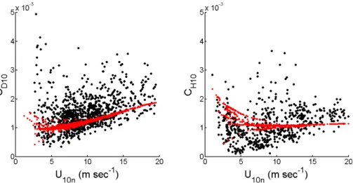
3.3 Transfer coefficients for momentum (C_D10_{) and sensible heat (}C_H10₎

15

Eddy covariance momentum and sensible heat fluxes were calculated from the Knorr_11 measurements using 10 min averaging intervals. Drag (C_D10) and sensible heat (CH10) transfer coefficient values were calculated from the data following Kondo

(1975). Knorr_11 CD10 shows a general increase from approximately 1.0×10− 3

to 1.5×10−3 as wind speeds increase from <5 m s−1 to 20 m s−1 (Fig. 5a). The

mea-20

sured transfer coefficients are in reasonable agreement with those calculated using the NOAA COARE model for the Knorr_11 conditions (Fig. 5a, b). Knorr_11CH10data

clus-ter around 1×10−3 with little or no wind speed dependence (Fig. 5b). NOAA COARE model heat transfer coefficients for these conditions exhibit a bias high at lower wind speeds and a bias low at the higher wind speeds. There is no evidence of suppression

25

of either momentum or sensible heat transfer coe_fficients under the high wind speed conditions during ST191.

(18)

ACPD

13, 13285–13322, 2013

Atlantic

T. G. Bell et al.

Title Page

Tables Figures

◭ ◮

Back Close

Full Screen / Esc

Discussion

P

a

per

|

Dis

cussion

P

a

per

|

Discussion

P

a

per

|

Discussio

n

P

a

per

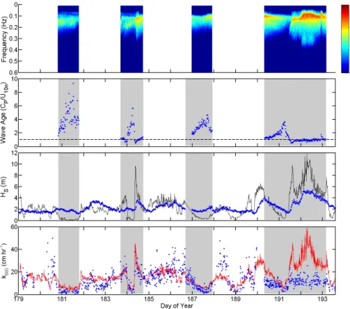
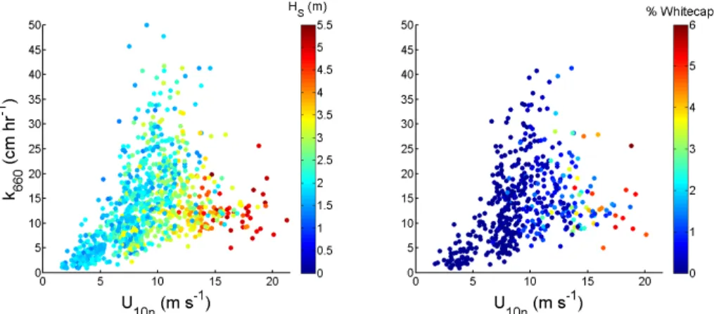
3.4 Waves, whitecaps and gas transfer

Wave spectra, wave age and significant wave height (HS) were examined to compare

the wave fields among the different stations occupied during the cruise (Fig. 6). Wave age was characterized asCP/U10n, where CP is the speed of the waves at the peak

frequency (older swell,CP/U10n>1; younger wind sea,CP/U10n≤1). The frequency of 5

the peak in the wave spectrum was similar at all stations, occurring between 0.05 and 0.3 Hz. Older swell was encountered during all four stations. Significant wave height (HS) rarely exceeded 3 m except during ST191 (Fig. 6c). During ST191 the wave field

was dominated by young waves which built rapidly fromHS=2 to 5 m as a result of

strong local winds (Fig. 6b). Even at intermediate winds (8–12 m s−1), consistently

10

larger wave heights occurred at ST191 compared to the other stations. During this period of strong winds and large, wind-driven waves,k660values (Fig. 6d) were

anoma-lously low wheneverHSexceeded 3 m (Fig. 7a).

Whitecap area coverage varied during the cruise from below detection to a maximum of about 5 %. Whitecaps exceeded 2 % on two occasions during the cruise. These

15

occurred during stations 184 and 191, associated with wind speeds exceeding 15 m s−1 and with young, wind-driven seas. Although the two stations exhibited similar whitecap coverage during their peak winds, significant wave height was nearly two-fold larger at station 191 (5 m maximum) than at station 184 (3 m maximum). The anomalous low DMS gas transfer coefficients observed during station 191 may therefore be more

20

directly linked to the appearance of large waves than to the onset of whitecaps (Fig. 7b).

4 Discussion

The data from Knorr_11 confirm the linear dependence ofkvs.Uat low to intermediate wind speeds observed in previous eddy covariance studies. This wind speed depen-dence appears to weaken at higher wind speeds in the presence of large waves. The

25

(19)

suggest-ACPD

13, 13285–13322, 2013

Atlantic

T. G. Bell et al.

Title Page

Tables Figures

◭ ◮

Back Close

Full Screen / Esc

Discussion

P

a

per

|

Dis

cussion

P

a

per

|

Discussion

P

a

per

|

Discussio

n

P

a

per

|

ing that gas transfer in the North Atlantic is not well described by a single monotonic relationship betweenk and mean wind speed (U10n). Most gas transfer

parameteriza-tions are based solely on the relaparameteriza-tionship betweenk and mean wind speed (U10n), but

it is widely recognized that gas transfer rates reflect a number of different processes that influence near surface turbulence and mixing (Wanninkhof et al., 2009). We

spec-5

ulate that variations in surfactants and/or wind/wave interactions are likely causes of variability ink vs.U in this study.

Laboratory studies have shown that gas transfer is related to the presence and mi-crobreaking of small-scale waves (Ocampo-Torres et al., 1994; Jähne et al., 1987; Zappa et al., 2004). Small-scale wave properties are primarily wind-driven, but they

10

can also be modulated by the presence of long waves (Donelan et al., 2010). Long waves and short waves are coupled through both hydrodynamic and wind-related pro-cesses. This coupling has a significant impact on air/sea transfer of momentum and it must also influence gas transfer. There has been little study of this phenomenon with regard to gas transfer, although a recent wind/wave tank study showed

suppres-15

sion of DMS gas transfer induced by superimposing mechanically-generated waves on a wind-generated wave field (Rhee et al., 2007). The presence of long waves may affect gas transfer of different gases to different extents. For example, gas transfer of CO2 is highly sensitive to large wave breaking and bubble formation. By contrast,

bubble-mediated exchange of the more soluble DMS is minor, and DMS is likely more

20

strongly influenced by processes that affect small-scale interfacial turbulence (Woolf, 1997; Blomquist et al., 2006).

It is interesting that k660 showed evidence of suppression at high wind speeds

dur-ing Knorr_11 at ST191 (Fig. 4), while the transfer coefficients for sensible heat did not (Fig. 5b). Sensible heat transfer is entirely air-side controlled. This difference in

be-25

haviour indicates that air-side turbulence increased strongly with wind speed, while the interfacial stress controlling DMS flux did not. Laboratory studies have suggested that air flow separation at the crests of large waves can effectively shield the troughs from wind stress (Reul et al., 1999, 2008; Veron et al., 2007). This could reduce surface

(20)

ACPD

13, 13285–13322, 2013

Atlantic

T. G. Bell et al.

Title Page

Tables Figures

◭ ◮

Back Close

Full Screen / Esc

Discussion

P

a

per

|

Dis

cussion

P

a

per

|

Discussion

P

a

per

|

Discussio

n

P

a

per

stress at the sea surface and increase waterside resistance (thereby reducingk660). In

this scenario, the sensible heat results suggest that sufficient atmospheric turbulence must be associated with the flow separation process to maintain strong atmospheric mixing even while surface stress is reduced.

The modulation of surface ocean turbulence by large gravity waves has been

incor-5

porated into some physical process-based surface renewal and energy dissipation gas transfer models (Soloviev et al., 2007; Soloviev, 2007; Soloviev and Schlussel, 1994). Soloviev (2007) used the dimensionless Keulegan number to scale the relationship between tangential and total surface stress:

K e=u3_∗/g.ν (7)

10

whereu∗is water side friction velocity,νis seawater viscosity, andgis gravity (Csanady,

1978). In this model, the relationship between total surface wind stress and tangential surface wind stress is given by:

τtangential=

τ_total

1+_{K e}K e_CR (8)

whereKeCRis based on the wave breaking parameterization of Zhao and Toba (2001). 15

This leads to a formulation that linksKe_CR (and interfacial gas transfer) to wave age, peak frequency, or significant wave height (Soloviev et al., 2007). The same wave breaking parameterization has also been used to describe the sea state-dependence of gas transfer by bubbles (Woolf, 2005; Soloviev et al., 2007; Zhao et al., 2003). Sim-ulations of the conditions during the Knorr_11 cruise illustrate the potential sensitivity

20

of gas transfer to the presence of long waves and to wave age (Fig. 8). The bubble-mediated transfer term is a small contribution tokDMSso the sensitivity of gas transfer

to wave age results primarily from changes in interfacial transfer.

Organic surfactants on the sea surface o_ffer an alternate explanation for wide vari-ations ink vs. wind speed. Surfactants modify the viscoelastic properties of seawater

(21)

ACPD

13, 13285–13322, 2013

Atlantic

T. G. Bell et al.

Title Page

Tables Figures

◭ ◮

Back Close

Full Screen / Esc

Discussion

P

a

per

|

Dis

cussion

P

a

per

|

Discussion

P

a

per

|

Discussio

n

P

a

per

|

and suppress surface turbulence. This, in turn, suppresses the formation of small-scale waves and reduces gas transfer (Salter et al., 2011; Frew et al., 1990). Marine surfac-tants are related to the abundance and chemistry of biologically-generated organic matter in the water column and to wave breaking, as surfactants are transported to the sea surface via bubbles. It is believed that surfactants can influence gas transfer at

5

all wind speeds, both by influencing interfacial transfer and by altering bubble surface properties (Wurl et al., 2011). The effect of surfactants has not yet been incorporated into gas transfer models, presumably because of the lack of information about their distribution and properties. There were no measurements of surfactant properties on Knorr_11 and thus we cannot quantify their effect upon gas exchange during this study.

10

5 Conclusions

The data from Knorr_11 demonstrate that eddy covariance DMS flux measurements, in conjunction with continuous seawater measurements, have the potential to capture variability in air/sea fluxes on sufficiently short time scales to resolve underlying pro-cesses if the relevant physical measurements are available. The relatively high

solu-15

bility of DMS makes the flux sensitive to the interfacial component of gas transfer and relatively insensitive to the bubble-mediated component (Blomquist et al., 2006). For this reason DMS fluxes are a useful tool for understanding near-surface turbulence and the factors that control interfacial exchange.

The weak dependence ofkDMSvs.U at high wind speeds observed during this cruise

20

was unexpected. There is one previous report of anomalously lowkDMSvalues at high

wind speeds for a limited portion of the Southern Ocean GasEx cruise (Yang et al., 2011; Vlahos et al., 2010). Vlahos et al. (2010) explained this phenomenon in terms of a reduction in effective solubility due to surface activity on bubbles, but this expla-nation appears unlikely given the small areal coverage of whitecaps observed during

25

Knorr_11. The weakened wind speed-dependence on Knorr_11 was associated with the presence of large wind-driven waves, but was less directly linked to the onset of

(22)

ACPD

13, 13285–13322, 2013

Atlantic

T. G. Bell et al.

Title Page

Tables Figures

◭ ◮

Back Close

Full Screen / Esc

Discussion

P

a

per

|

Dis

cussion

P

a

per

|

Discussion

P

a

per

|

Discussio

n

P

a

per

wave breaking and whitecap formation. We offer wind/wave coupling as an alternative explanation. However, we stress the need for additional field measurements to validate our observations and confirm that lowkDMS at high wind speeds is in fact a real

en-vironmental phenomenon and not an experimental artefact of unknown origin. Future studies should focus on simultaneous measurement of gas transfer, directional wave

5

fields, surface tension, surfactant properties and turbulence.

Supplementary material related to this article is available online at: http://www.atmos-chem-phys-discuss.net/13/13285/2013/

acpd-13-13285-2013-supplement.pdf.

Acknowledgements. The authors thank the Woods Hole Marine Department and the Captain 10

and crew of the R/V Knorr for their assistance in carrying out this cruise. We also thank Dan Repeta (WHOI) for pigment analysis and David Woolf, Chris Zappa and Mingxi Yang for in-sightful discussion. This research was supported by the NSF Atmospheric Chemistry Program (Grant Nos. 0851068, 0851472, 0851407 and 1134709) and is a contribution to US SOLAS. Wave sensor construction and the work of K. C. were supported by the Research Council of 15

Norway (Grant No. 196438, BIOWAVE). B. W. acknowledges support from science foundation Ireland under grant 08/US/I1455 and from the FP7 Marie Curie Reintegration programme under Grant 224776.

References

Alves, J., Banner, M. L., and Young, I. R.: Revisiting the Pierson–Moskowitz asymptotic limits 20

for fully developed wind waves, J. Phys. Oceanogr., 33, 1301–1323, 2003.

Bandy, A. R., Thornton, D. C., Tu, F. H., Blomquist, B. W., Nadler, W., Mitchell, G. M., and Lenschow, D. H.: Determination of the vertical flux of dimethyl sulfide by eddy correlation and atmospheric pressure ionization mass spectrometry (APIMS), J. Geophys. Res.-Atmos., 107, 4743, doi:10.1029/2002jd002472, 2002.

(23)

ACPD

13, 13285–13322, 2013

Atlantic

T. G. Bell et al.

Title Page

Tables Figures

◭ ◮

Back Close

Full Screen / Esc

Discussion

P

a

per

|

Dis

cussion

P

a

per

|

Discussion

P

a

per

|

Discussio

n

P

a

per

|

Bange, H. W., Bell, T. G., Cornejo, M., Freing, A., Uher, G., Upstill-Goddard, R. C., and Zhang, G.: MEMENTO: a proposal to develop a database of marine nitrous oxide and methane measurements, Environ. Chem., 6, 195–197, 2009.

Blomquist, B. W., Fairall, C. W., Huebert, B. J., Kieber, D. J., and Westby, G. R.: DMS sea–air transfer velocity: direct measurements by eddy covariance and parameteriza-5

tion based on the NOAA/COARE gas transfer model, Geophys. Res. Lett., 33, L07601, doi:10.1029/2006gl025735, 2006.

Blomquist, B. W., Huebert, B. J., Fairall, C. W., and Faloona, I. C.: Determining the sea–air flux of dimethylsulfide by eddy correlation using mass spectrometry, Atmos. Meas. Tech., 3, 1–20, doi:10.5194/amt-3-1-2010, 2010.

10

Broecker, W. S., Peng, T. H., Ostlund, G., and Stuiver, M.: The distribution of bomb radiocarbon in the ocean, J. Geophys. Res.-Oceans, 90, 6953–6970, 1985.

Butler, J. H., Bell, T. G., Hall, B. D., Quack, B., Carpenter, L. J., and Williams, J.: Technical Note: Ensuring consistent, global measurements of very short-lived halocarbon gases in the ocean and atmosphere, Atmos. Chem. Phys., 10, 327–330, doi:10.5194/acp-10-327-2010, 2010. 15

Callaghan, A. H. and White, M.: Automated processing of sea surface images for the determination of whitecap coverage, J. Atmos. Ocean. Tech., 26, 383–394, doi:10.1175/2008jtecho634.1, 2009.

Christensen, K. H., Röhrs, R., Ward, B., Drivdal, M., and Broström, G.: Surface wave measure-ments using a ship mounted ultrasonic altimeter, ASLO Ocean Sciences Meeting, abstract 20

no. 10981, 21 February 2012, Salt Lake City, USA, 2012.

Csanady, G. T.: Turbulent interface layers, J. Geophys. Res., 83, 2329–2342, 1978.

Dacey, J. W. H., Wakeham, S. G., and Howes, B. L.: Henry’s law constants for dimethylsulfide in fresh water and seawater, Geophys. Res. Lett., 11, 991–994, 1984.

Donelan, M. A., Haus, B. K., Plant, W. J., and Troianowski, O.: Modulation of short wind waves 25

by long waves, J. Geophys. Res.-Oceans, 115, C10003, doi:10.1029/2009jc005794, 2010. Edson, J. B., Hinton, A. A., Prada, K. E., Hare, J. E., and Fairall, C. W.: Direct covariance flux

estimates from mobile platforms at sea, J. Atmos. Ocean. Technol., 15, 547–562, 10.1175/ 1520-0426(1998)015<0547:DCFEFM>2.0, 1998.

Elliott, S.: Dependence of DMS global sea–air flux distribution on transfer velocity and con-30

centration field type, J. Geophys. Res.-Biogeo., 114, G02001, doi:10.1175/1520-0426(1998) 015<0547:DCFEFM>2.0.CO;2, 2009.

(24)

ACPD

13, 13285–13322, 2013

Atlantic

T. G. Bell et al.

Title Page

Tables Figures

◭ ◮

Back Close

Full Screen / Esc

Discussion

P

a

per

|

Dis

cussion

P

a

per

|

Discussion

P

a

per

|

Discussio

n

P

a

per

Fairall, C. W., Bradley, E. F., Rogers, D. P., Edson, J. B., and Young, G. S.: Bulk parameteri-zation of air–sea fluxes for Tropical Ocean-Global Atmosphere Coupled-Ocean Atmosphere Response Experiment, J. Geophys. Res.-Oceans, 101, 3747–3764, 1996.

Fairall, C. W., Yang, M., Bariteau, L., Edson, J. B., Helmig, D., McGillis, W., Pezoa, S., Hare, J. E., Huebert, B., and Blomquist, B.: Implementation of the Coupled Ocean-5

Atmosphere Response Experiment flux algorithm with CO₂, dimethyl sulfide, and O₃, J. Geophys. Res.-Oceans, 116, C10003, doi:10.1029/2010jc006884, 2011.

Frew, N. M., Goldman, J. C., Dennett, M. R., and Johnson, A. S.: Impact of phytoplankton-generated surfactants on air–sea gas exchange, J. Geophys. Res.-Oceans, 95, 3337–3352, 1990.

10

García-Nava, H., Ocampo-Torres, F. J., Osuna, P., and Donelan, M. A.: Wind stress in the presence of swell under moderate to strong wind conditions, J. Geophys. Res.-Oceans, 114, C00J11, doi: doi:10.1175/1520-0426(1998)015<0547:DCFEFM>2.0.CO;2, 2009.

García-Nava, H., Ocampo-Torres, F. J., Hwang, P. A., and Osuna, P.: Reduction of wind stress due to swell at high wind conditions, J. Geophys. Res.-Oceans, 117, C12008, 15

doi:10.1029/2008JG000710, 2012.

Hare, J. E., Fairall, C. W., McGillis, W. R., Edson, J. B., Ward, B., and Wanninkhof, R.: Evalu-ation of the NEvalu-ational Oceanic and Atmospheric AdministrEvalu-ation/Coupled-Ocean Atmospheric Response Experiment (NOAA/COARE) air–sea gas transfer parameterization using GasEx data, J. Geophys. Res.-Oceans, 109, C08S11, doi:10.1029/2003JC001831, 2004.

20

Harman-Fetcho, J. A., McConnell, L. L., Rice, C. P., and Baker, J. E.: Wet deposition and air-water gas exchange of currently used pesticides to a subestuary of the Chesapeake Bay, Environ. Sci. Technol., 34, 1462–1468, doi:10.1021/Es990955l, 2000.

Ho, D. T., Law, C. S., Smith, M. J., Schlosser, P., Harvey, M., and Hill, P.: Measurements of air–sea gas exchange at high wind speeds in the Southern Ocean: implications for global 25

parameterizations, Geophys. Res. Lett., 33, L16611, doi:10.1029/2009JC005389, 2006. Huebert, B. J., Blomquist, B. W., Hare, J. E., Fairall, C. W., Johnson, J. E., and Bates, T. S.:

Measurement of the sea–air DMS flux and transfer velocity using eddy correlation, Geophys. Res. Lett., 31, L23113, doi:10.1029/2011JC007833, 2004.

Huebert, B. J., Blomquist, B. W., Yang, M. X., Archer, S. D., Nightingale, P. D., Yelland, M. J., 30

(25)

ACPD

13, 13285–13322, 2013

Atlantic

T. G. Bell et al.

Title Page

Tables Figures

◭ ◮

Back Close

Full Screen / Esc

Discussion

P

a

per

|

Dis

cussion

P

a

per

|

Discussion

P

a

per

|

Discussio

n

P

a

per

|

Jähne, B., Munnich, K. O., Bosinger, R., Dutzi, A., Huber, W., and Libner, P.: On the parameters influencing air-water gas-exchange, J. Geophys. Res.-Oceans, 92, 1937–1949, 1987. Johnson, M. T.: A numerical scheme to calculate temperature and salinity dependent air-water

transfer velocities for any gas, Ocean Sci., 6, 913–932, doi:10.5194/os-6-913-2010, 2010. Johnson, M. T., Liss, P. S., Bell, T. G., Lesworth, T. J., Baker, A. R., Hind, A. J., Jick-5

ells, T. D., Biswas, K. F., Woodward, E. M. S., and Gibb, S. W.: Field observations of the ocean-atmosphere exchange of ammonia: fundamental importance of temperature as re-vealed by a comparison of high and low latitudes, Global Biogeochem. Cy., 22, GB1019, doi:10.1029/2007GB003039, 2008.

Juranek, L. W., Hamme, R. C., Kaiser, J., Wanninkhof, R., and Quay, P. D.: Evidence of O₂ con-10

sumption in underway seawater lines: implications for air-sea O₂and CO₂fluxes, Geophys. Res. Lett., 37, L01601, doi:10.1029/2009GL040423, 2010.

Kondo, J.: Air-sea bulk transfer coe_fficients in diabatic conditions, Bound.-Lay. Meteorol., 9, 91– 112, 1975.

Lana, A., Bell, T. G., Simó, R., Vallina, S. M., Ballabrera-Poy, J., Kettle, A. J., Dachs, J., Bopp, L., 15

Saltzman, E. S., Stefels, J., Johnson, J. E., and Liss, P. S.: An updated climatology of surface dimethylsulfide concentrations and emission fluxes in the global ocean, Global Biogeochem. Cy., 25, GB1004, doi:10.1029/2010GB003850, 2011.

Lenschow, D. H. and Raupach, M. R.: The attenuation of fluctuations in scalar con-centrations through sampling tubes, J. Geophys. Res.-Atmos., 96, 15259–15268, 20

doi:10.1029/91jd01437, 1991.

Liss, P. S. and Merlivat, L.: Air–sea gas exchange rates: introduction and synthesis, in: The Role of Air–Sea Exchange in Geochemical Cycling, edited by: Buatmenard, P., Reidel, Norwell, Mass., USA, 113–127, 1986.

Liss, P. S. and Slater, P. G.: Flux of gases across the air–sea interface, Nature, 247, 181–184, 25

1974.

Longhurst, A.: Seasonal cycles of pelagic production and consumption, Prog. Oceanogr., 36, 77–167, 1995.

Marandino, C. A., De Bruyn, W. J., Miller, S. D., and Saltzman, E. S.: Eddy correlation mea-surements of the air/sea flux of dimethylsulfide over the North Pacific Ocean, J. Geophys. 30

Res.-Atmos., 112, D03301, doi:10.1029/2006JD007293, 2007.

(26)

ACPD

13, 13285–13322, 2013

Atlantic

T. G. Bell et al.

Title Page

Tables Figures

◭ ◮

Back Close

Full Screen / Esc

Discussion

P

a

per

|

Dis

cussion

P

a

per

|

Discussion

P

a

per

|

Discussio

n

P

a

per

Marandino, C. A., De Bruyn, W. J., Miller, S. D., and Saltzman, E. S.: DMS air/sea flux and gas transfer coefficients from the North Atlantic summertime coccolithophore bloom, Geophys. Res. Lett., 35, L23812, doi:10.1029/2008GL036370, 2008.

Marandino, C. A., De Bruyn, W. J., Miller, S. D., and Saltzman, E. S.: Open ocean DMS air/sea fluxes over the eastern South Pacific Ocean, Atmos. Chem. Phys., 9, 345–356, 5

doi:10.5194/acp-9-345-2009, 2009.

Massman, W. J.: A simple method for estimating frequency response corrections for eddy co-variance systems, Agr. Forest Meteorol., 104, 185–198, doi:10.1016/S0168-1923(00)00164-7, 2000.

McGillis, W. R., Dacey, J. W. H., Frew, N. M., Bock, E. J., and Nelson, R. K.: Water–air flux of 10

dimethylsulfide, J. Geophys. Res.-Oceans, 105, 1187–1193, 2000.

McGillis, W. R., Edson, J. B., Hare, J. E., and Fairall, C. W.: Direct covariance air–sea CO₂ fluxes, J. Geophys. Res.-Oceans, 106, 16729–16745, 2001.

McGillis, W. R., Edson, J. B., Zappa, C. J., Ware, J. D., McKenna, S. P., Terray, E. A., Hare, J. E., Fairall, C. W., Drennan, W., Donelan, M., DeGrandpre, M. D., Wanninkhof, R., 15

and Feely, R. A.: Air-sea CO₂exchange in the equatorial Pacific, J. Geophys. Res.-Oceans, 109, C08S02, doi:10.1029/2003JC002256, 2004.

Miller, S. D., Hristov, T. S., Edson, J. B., and Friehe, C. A.: Platform motion effects on measure-ments of turbulence and air–sea exchange over the open ocean, J. Atmos. Ocean. Tech., 25, 1683–1694, 2008.

20

Miller, S. D., Marandino, C., and Saltzman, E. S.: Ship-based measurement of air– sea CO₂ exchange by eddy covariance, J. Geophys. Res.-Atmos., 115, D02304, doi:10.1029/2009JD012193, 2010.

Nightingale, P. D., Malin, G., Law, C. S., Watson, A. J., Liss, P. S., Liddicoat, M. I., Boutin, J., and Upstill-Goddard, R. C.: In situ evaluation of air–sea gas exchange parameterizations using 25

novel conservative and volatile tracers, Global Biogeochem. Cy., 14, 373–387, 2000. Ocampo-Torres, F. J., Donelan, M. A., Merzi, N., and Jia, F.: Laboratory measurements of mass

transfer of carbon dioxide and water vapor for smooth and rough flow conditions, Tellus B, 46, 16–32, doi:10.1034/j.1600-0889.1994.00002.x, 1994.

Pedreros, R., Dardier, G., Dupuis, H., Graber, H. C., Drennan, W. M., Weill, A., Guerin, C., and 30