Analysis and Prediction of the Metabolic Stability of
Proteins Based on Their Sequential Features, Subcellular
Locations and Interaction Networks
Tao Huang1,2, Xiao-He Shi4, Ping Wang4, Zhisong He5, Kai-Yan Feng2, LeLe Hu3, Xiangyin Kong4,6*, Yi-Xue Li1,2*, Yu-Dong Cai3,7,8*, Kuo-Chen Chou8*
1Key Laboratory of Systems Biology, Shanghai Institutes for Biological Sciences, Chinese Academy of Sciences, Shanghai, People’s Republic of China,2Shanghai Center for Bioinformation Technology, Shanghai, People’s Republic of China,3Institute of Systems Biology, Shanghai University, Shanghai, People’s Republic of China,4Institute of Health Sciences, Shanghai Institutes for Biological Sciences, Chinese Academy of Sciences and Shanghai Jiao Tong University School of Medicine, Shanghai, People’s Republic of China,5CAS-MPG Partner Institute for Computational Biology, Shanghai Institutes for Biological Sciences, Chinese Academy of Sciences, Shanghai, People’s Republic of China,6State Key Laboratory of Medical Genomics, Ruijin Hospital, Shanghai Jiaotong University, Shanghai, People’s Republic of China,7Centre for Computational Systems Biology, Fudan University, Shanghai, People’s Republic of China,8Gordon Life Science Institute, San Diego, California, United States of America
Abstract
The metabolic stability is a very important idiosyncracy of proteins that is related to their global flexibility, intramolecular fluctuations, various internal dynamic processes, as well as many marvelous biological functions. Determination of protein’s metabolic stability would provide us with useful information for in-depth understanding of the dynamic action mechanisms of proteins. Although several experimental methods have been developed to measure protein’s metabolic stability, they are time-consuming and more expensive. Reported in this paper is a computational method, which is featured by (1) integrating various properties of proteins, such as biochemical and physicochemical properties, subcellular locations, network properties and protein complex property, (2) using the mRMR (Maximum Relevance & Minimum Redundancy) principle and the IFS (Incremental Feature Selection) procedure to optimize the prediction engine, and (3) being able to identify proteins among the four types: ‘‘short’’, ‘‘medium’’, ‘‘long’’, and ‘‘extra-long’’ half-life spans. It was revealed through our analysis that the following seven characters played major roles in determining the stability of proteins: (1) KEGG enrichment scores of the protein and its neighbors in network, (2) subcellular locations, (3) polarity, (4) amino acids composition, (5) hydrophobicity, (6) secondary structure propensity, and (7) the number of protein complexes the protein involved. It was observed that there was an intriguing correlation between the predicted metabolic stability of some proteins and the real half-life of the drugs designed to target them. These findings might provide useful insights for designing protein-stability-relevant drugs. The computational method can also be used as a large-scale tool for annotating the metabolic stability for the avalanche of protein sequences generated in the post-genomic age.
Citation:Huang T, Shi X-H, Wang P, He Z, Feng K-Y, et al. (2010) Analysis and Prediction of the Metabolic Stability of Proteins Based on Their Sequential Features, Subcellular Locations and Interaction Networks. PLoS ONE 5(6): e10972. doi:10.1371/journal.pone.0010972
Editor:Andreas Hofmann, Griffith University, Australia
ReceivedMarch 29, 2010;AcceptedMay 14, 2010;PublishedJune 4, 2010
Copyright:ß2010 Huang et al. This is an open-access article distributed under the terms of the Creative Commons Attribution License, which permits unrestricted use, distribution, and reproduction in any medium, provided the original author and source are credited.
Funding:This work was supported by grants from the National High Technology Research and Development Program of China (2006AA02A301), the National Basic Research Program of China (No. 2007CB512202), the Knowledge Innovation Program of the Chinese Academy of Sciences (Grant No. KSCX1-YW-R-74) and Key Research Program (CAS) (KSCX2-YW-R-112). The funders had no role in study design, data collection and analysis, decision to publish, or preparation of the manuscript.
Competing Interests:The authors have declared that no competing interests exist.
* E-mail: [email protected] (XYK); [email protected] (YXL); [email protected] (YDC); [email protected] (KCC)
Introduction
Proteins are inherently dynamic molecules of marginal stability. Many marvelous biological functions of proteins are realized through their internal motions [1,2,3,4]. The physicochemical stability and flexibility are balanced with each other. They are also thought as intimately correlated with their intramolecular fluctuations and various other dynamic processes [5]. Protein flexibility facilitates adaptation and recognition [6] in diverse molecular events, such as switch between active and inactive states [7], allosteric transition [8], intercalation of drugs into DNA [9], cooperative effects [10], and assembly of microtubules [11]. It is also essential for in-depth understanding the M2 proton channel gating and inhibition mechanism [3,12,13,14], the switch mechanism of human Rab5a [15], the inhibition mechanism of
PTP1B [16], the metabolic mechanism [17], and the action mechanism of calmodulin [18,19]. These properties present unique challenges to the pharmaceutical scientists attempting to develop protein-stability-relevant drugs [20,21,22].
Traditional methods of measuring protein’s metabolic stability rely on either pulse-chase metabolic labeling or administration of protein synthesis inhibitors followed by half-life biochemical analysis of the abundance of the protein concerned at multiple time points during the chase period. Highly regulated proteins tend to be present in low amounts. Since even mass spectrometry plus failed to detect low-abundance proteins, study about protein’s metabolic stability remains far from complete yet although it is of critical importance for drug development. Recently, it was reported that high-throughput systematic approaches for the analysis of global metabolic stability were taken by using a
fluorescence-based system to monitor metabolic stability at the single-cell level [23]. In this regard, however, computational approaches would be much more efficient not only in timely providing the information about the stability of query proteins but also in helping analyze what factors play major roles to the metabolic stability. This study was initiated in an attempt to develop a computational method for investigating the metabolic stability of proteins in terms of their biochemical and physico-chemical properties or features. Our results suggest that KEGG enrichment scores, subcellular locations, polarity, amino acids composition, hydrophobicity, secondary structure propensity, and number of protein complexes, play irreplaceable roles for protein’s metabolic stability. Moreover, we predicted the metabolic stability of drug target proteins using the selected features and found an intriguing correlation between the predicted metabolic stability of some proteins and the real half-life of the drugs designed to target them.
Materials and Methods
Data set
As elucidated in a recent review [24], to develop an effective statistical method for predicting protein attributes, one of the indispensable things is a valid benchmark dataset. Here, protein stability data were taken from Yen’s work [23]. We downloaded ORFs from hORFeome v5.1 library (http://horfdb.dfci.harvard. edu/), and translated ORFs to protein sequences using transeq in Emboss [25]. Proteins with the length shorter than 50 and longer than 2700, were excluded. In Yen’s work, protein samples were divided into four groups according to their PSI (protein stability index): (1) short half-life (PSI,2), (2) medium half-life (2#PSI,3), (3) long half-life (3#PSI,4), and (4) extra-long half-life (PSI$4). After being thus processed, our dataset consist of 223 short half-life proteins, 446 medium half-life proteins, 706 long half-life proteins and 496 extra-long half-life proteins. For reader’s convenience, these sequences (classified into above four groups) are given in Dataset S1.
Biochemical and physicochemical description of proteins In order to formulate protein samples of different sequence lengths with vectors of a uniform dimension, let us adopt the concept of pseudo amino acid composition (PseAAC) [24,26,27]. The concrete procedures are that the biochemical and physico-chemical properties [28,29,30,31] are singled out from a protein sequence according to the following seven aspects: (1) amino acid composition (AAC) [32], (2) secondary structure propensity, (3) hydrophobicity, (4) polarizability, (5) solvent accessibility, (6) normalized van der Waals volume, and (7) polarity [33].
Of the above seven types of properties, except for AAC (the occurrence frequencies of the 20 native amino acids for a given protein [34]) that is an extensive quantity reflecting the global or overall feature of a protein, all the other six types are associated with a single amino acid in a given protein sequence position and hence belong to a localized quantity.
The six local types of properties can each be classified into two or three categories. For example, for the secondary structure propensity, each amino acid can be classified as: helix, strand or coil, as predicted by SSpro [35]. For solvent accessibility: buried or exposed to solvent, as predicted by ACCpro [36]. For the other four types of properties, i.e., hydrophobicity, polarizability, normalized van der Waals volume and polarity, each of the constituent amino acids can also be classified into three categories in a similar way according to their values. In terms of hydrophobicity, there are three groups of amino acid: polar (R, K, E, D, Q, N), neutral (G, A, S, T, P, H, Y) and hydrophobic (C, V, L, I, M, F, W) [37]. In terms
of polarizability, there are three groups of amino acid: 0–0.108 (G, A, S, D, T), 0.128–0.186 (C, P, N, V, E, Q, I, L) and 0.219–0.409 (K, M, H, F, R, Y, W) [38]. In terms of normalized van der Waals volume, there are three groups of amino acid: 0–2.78 (G, A, S, C, T, P, D), 2.95–4.0 (N, V, E, Q, I, L) and 4.43–8.08 (M, H, K, F, R, Y, W) [38]. In terms of polarity, there are three groups of amino acid: 4.9–6.2 (L, I, F, W, C, M, V, Y), 8.0–9.2 (P, A, T, G, S) and 10.4– 13.0 (H, Q, R, K, N, E, D) [39].
Now, the problem is how to generate the corresponding global quantity by integrating the localized quantities over an entire protein sequence. To realize this, let us consider the hydropho-bicity first. In this study, the hydrophohydropho-bicity of an amino acid is classified as: P (polar), N (neutral), or H (hydrophobic). Thus, for a protein sequence, say, ‘‘MSDKPDMAEIEKFSKETIEQEKQA-GESTQEKNPLPMLLPATDKSKLKKTE’’, it can be coded as ‘‘HNPPNPHNPHPPHNPPNHPPPPPNNPNNPPPPNHNHHH-NNNPPNPHPPNP’’.
For the above coded sequence, the following three extensive quantities can be derived:C(composition),T (transition), andD (distribution).Crefers to the global percent composition of each of the three groups (i.e., P, N, and H) in the coded sequence;Tto the percent frequencies with which the code letter changes to another along the entire length of the coded sequence; and D to the distribution pattern of the code letters along the sequence, measuring the percentage of the sequence length within which the first, 25%, 50%, 75%, and 100% of each of the three code letters is located.
Take the above coded sequence of 50 letters as an example. It is composed of 10 Hs, 16 Ns and 24 Ps, as shown in Figure 1. Thus, we have the composition C= (10/50 = 20.0%, 16/ 50 = 32%, 24/50 = 48%) for H, N and P respectively. For the transition feature T, there are totally 31 transitions in the sequence, with 8 between H and N, 16 between N and P, and 7 between H and P, so that we have T= (8/31 = 25.81%, 16/ 31 = 51.61% and 7/31 = 22.58%). As for the distributionD, the first, 25%, 50%, 75% and 100% of H are located at the positions of 1st, 10th, 18th, 37th, and 46th in the coded sequence, respectively. Thus, the distribution D for H is 1/50 = 2%, 10/ 50 = 20%, 18/50 = 36%, 37/50 = 74%, and 46/50 = 92%. Like-wise, the distributionDfor N is 4%, 28%, 54%, 78%, and 98%; and that for P is 6%, 24%, 44%, 64%, and 100%. Accordingly, we haveD= (2%, 20%, 36%, 74%, 92%, 4%, 28%, 54%, 78%, 98%, 6%, 24%, 44%, 64%, and 100%). CombiningC,T andD, we have a total of 21 elements.
For the ‘‘secondary structure’’, ‘‘polarizability’’, ‘‘normalized van der Waals volume’’ and ‘‘polarity’’, each of them is also classified into three categories and hence would also generate21 elements in a similarly way as described above for the case of ‘‘hydrophobicity’’.
For the ‘‘solvent accessibility’’, since it is classified into two categories, the combination ofC,TandDfor the sequence coded according to the ‘‘solvent accessibility’’ would only generate 7 elements rather than 21.
Now for the ‘‘AAC’’ we have 20 elements [34]; for the ‘‘solvent accessibility’’, 7 elements; and for each of all the other five types of protein properties, 21 elements. Combining all these extensive quantities together, we have an augmented extensive quantity containing (5621+20+7) = 132 elements, as listed inTable 1for the details. Furthermore, some more elements should also be included as will be illustrated below.
Subcellular location description of proteins
improved by incorporating the protein subcellular location information. Unfortunately, only a small amount of proteins have subcellular locations annotated in UniProt [42]. To make up this, the subcellular locations for most proteins were predicted based on the sequence similarity evaluated by BLAST [43]. If the BLAST score of a query protein with a location-known protein was greater than 120, they were considered similar with the query protein. The subcellular locations of the query protein were the intersection of subcellular locations of its sequence similar location-known proteins. Since there were 22 subcellular locations, the subcellular location features of each protein can be represented by a 22-dimensional vector, namely L~(‘1,‘2,‘3,:::,‘22), where ‘i~1if the protein is located at thei-thsubcellular location site; otherwise,‘i~0. It is instructive to point out that one can also use the web-server predictor Euk-mPLoc [44] to get the desired information for those proteins without subcellular location annotated in UniProt database. The updated website address for Euk-mPLoc can be found in the Cell-PLoc package [41] as well as in Table 3 of [45]. The good thing about Euk-mPLoc is that it not only can cover up to 22 subcellular location sites but is also able to identify proteins with multiple location sites, which is particularly useful for drug development as elaborated recently by Smith [46].
KEGG enrichment scores of proteins
The simplest and most direct method for predicting the function of a query protein based on the training dataset of function-known proteins is the immediate neighborhood method [47]. The information of the neighbor proteins is also an important environmental feature to the protein concerned. Actually, the neighbor proteins are in interaction with each other in the STRING network [48]. The KEGG enrichment score of the protein and its neighbors was defined as the2log10of the p value generated by hypergeometric test on KEGG pathway. The larger enrichment score means more overrepresentation. There were 220 KEGG enrichment scores for each of the proteins investigated here.
Number of protein complexes
If a protein can form a complex with other proteins, it will be more stable and have longer half-life. Therefore, the number of this kind of complexes a protein can form is a feature relevant to its stability, and should be counted in prediction as well. We downloaded the protein complex dataset from CORUM [49], which is a comprehensive resource of mammalian protein complexes.
Feature space of proteins
As mentioned above, the 7 types of biochemical and physicochemical properties would contribute 132 components to describe a protein. In addition, its length could also be counted as a component, its occurrences in the 22 subcellular location sites as 22 components, its 220 KEGG enrichment scores as 220 components, and its number in forming protein-protein complexes as a component, the total components used in this study to represent a protein sample would be (132+1+22+220+1) = 376 components. For the list of the 376 feature components, see the Table S1.
Thus, the i-th protein sample Pi should be formulated as a vector in a 376-D (dimensional) space; i.e.,
Pi~ pi
1 pi2 ::: pi375 pi376
T ð1Þ
wherepi
jis thej-th (j~1,2,:::,376)component of thei-thprotein sample Pi and can be derived by following the procedures as elaborated above.
Note that before performing prediction, each of the 376 components in Eq.1 should undergo the following standard conversion procedure:
pi
jZ(pij{mj)=sj (i~1,2,:::,N; j~1,2,:::,376) ð1aÞ whereNis the number of the total proteins in the training dataset,
mj~P N
i~1
pi
j=N and sj~
ffiffiffiffiffiffiffiffiffiffiffiffiffiffiffiffiffiffiffiffiffiffiffiffiffiffiffiffiffiffiffi PN
i~1 (pi
j{mj)2=N s
are the mean and
standard deviation of the j-th component over the N protein samples. The converted values obtained by Eq.1a will have a zero mean value over the N protein samples, and will remain unchanged if going through the same conversion procedure again [24,26].
mRMR method
The ‘‘maximum relevance & minimum redundancy’’ (mRMR) method was originally developed by Peng et al. [50] to deal with the microarray data processing. In their method, each feature is ranked according to its relevance to the target and redundancy with other features. A ‘‘good’’ feature is defined as the one that has the best trade-off between maximizing the relevance to the target and minimizing the redundancy within the features. To quantify both the relevance and redundancy, the following mutual Figure 1. How to compute the 21 hydrophobic feature components from protein sequence.According to the hydrophobicity of each amino acid, the protein sequence ‘‘MSDKPDMAEIEKFSKETIEQEKQAGESTQEKNPLPMLLPATDKSKLKKTE’’ was converted to a hydrophobic sequence ‘‘HNPPNPHNPHPPHNPPNHPPPPPNNPNNPPPPNHNHHHNNNPPNPHPPNP’’. It is composed of 10 Hs, 16 Ns and 24 Ps. There are totally 31 transitions in the sequence, with 8 between H and N, 16 between N and P, and 7 between H and P. Based on the composition, transition, and distribution of H, N, P, 21 hydrophobic feature components of this protein can be calculated.
doi:10.1371/journal.pone.0010972.g001
Metabolic Stability Prediction
Table 1.The 132 biochemical and physicochemical feature components of proteins.
Biochemical and
physicochemical description
Vector index
Amino acid category
Protein Feature
category Protein Feature description
Number of vector components
Index of vector components
Total Number
Hydrophobicity V1:V21 P: r|k|e|d|q|n C(composition) Composition of P, N, H 3 V1:V3 21
N: g|a|s|t|p|h|y T(transition) Transition of PN, PH, NH 3 V4:V6
H: c|v|l|i|m|f|w D(distribution) Distribution of P, N, H 15 V7:V21
Secondary structure V22:V42 SSpro C(composition) Composition of H, E, C 3 V22:V24 21
H: helix T(transition) Transition of HE, HC, EC 3 V25:V27
E: strand D(distribution) Distribution of H, E, C 15 V28:V42
C:coil
Solvent accessibility V43:V49 ACCpro C(composition) Composition of H 1 V43 7
H: hidden T(transition) Transition of HE 1 V44
E: exposed D(distribution) Distribution of H 5 V45:V49
Normalized van der Waals volume V50:V70 H: g|a|s|c|t|d|p C(composition) Composition of H, E, C 3 V50:V52 21
E: n|v|e|q|i|l T(transition) Transition of HE, HC, EC 3 V53:V55
C:m|h|k|f|r|y|w D(distribution) Distribution of H, E, C 15 V56:V70
Polarity V71:V91 H: l|i|f|w|c|m|v|y C(composition) Composition of H, E, C 3 V71:V73 21
E: g|a|t|p|s T(transition) Transition of HE, HC, EC 3 V74:V76
C: h|q|r|k|n|e|d D(distribution) Distribution of H, E, C 15 V77:V91
Polarizability V92:V112 H: g|a|s|d|t C(composition) Composition of H, E, C 3 V92:V94 21
E: c|p|n|v|e|q|i|l T(transition) Transition of HE, HC, EC 3 V95:V97
C: k|m|h|f|r|y|w D(distribution) Distribution of H, E, C 15 V98:V112
Amino Acids Composition V113:V132 r, k, e, d, q, n, g, a, s, t, p, h, y, c, v, l, i, m, f, w
C(composition) 20 20
doi:10.1371/journal.pone.0010972.t001
Metabolic
Stability
Prediction
ONE
|
www.plos
one.org
4
June
2010
|
Volume
5
|
Issue
6
|
information (MI) is defined to estimate how one vector is related to another:
I(x,y)~ ðð
p(x,y) log p(x,y)
p(x)p(y)dxdy ð2Þ
wherex,yare two vectors,p(x,y)is the joint probabilistic density, p(x)andp(y)are the marginal probabilistic densities.
Suppose V denotes the entire space containing all the aforementioned 376 components, andVa(
5V)denotes the space containsacomponents selected fromV. The space to be identified is denoted byVb(
5V)that containsbcomponents. The relevance Rof the featuref inVbwith the targethcan be calculated by:
R~I(f,h) ð3Þ
And the redundancyDof the featuref inVbwith all the features inVacan be calculated by:
D~1
a
X
fi[Va
I(f,fi) ð4Þ
To obtain a feature fj in Vb with maximum relevance and minimum redundancy, Eqs.3 and 4 are combined with the mRMR function:
max
fj[Vb
I(fj,h){1
a
X
fi[Va
I(fj,fi)
2
4
3
5 (j~1,2,:::,b) ð5Þ
For a feature set with 376 (~azb) components, the feature evaluation will continue for 376 rounds. After these evaluations, a feature set S can be obtained by the mRMR method as formulated below:
S~ f10,f20,:::,fh0,:::,f3760
n o
ð6Þ
where each feature inShas an subscript index, indicating at which round that the feature is selected. The better a feature is, the earlier it will satisfy Eq.5 and be selected, and the smaller its subscript index will be.
Nearest Neighbor Algorithm
In our study, the Nearest Neighbor (NN) algorithm or NNA is used to classify a protein as either labile or a stable one. NNA makes its decision by calculating the ‘‘distances’’ of a query protein with all the proteins in the training dataset one-by-one. Varieties of distance scales can be used for this purpose, such as Euclidean distance [51], Hamming distance [52], and Mahalanobis distance [34]. In the current study, the distance between the query protein P andPi, thei-th protein in the training dataset, is defined by [53,54,55]:
D(P,Pi)~1{ P :Pi
DDPDD:DDPiDD ð7Þ
Where P and Pi are the feature component vector of query protein and thei-thprotein in the training dataset (cf. Eq.1);P:Pi is the inner product of P and Pi; k kP and Pi
represent the
modules of vectorsPand Pi. The smaller D(P,Pi)is, the more similarPtoPiis. According to the NN rule, given a training set Strain~P1,
P2,:::,Pm,:::,PV
, the query protein P will be predicted belonging to the same class ofPm that is the closest to P. In other words, if
m~arg miniD(P,Pi) ð8Þ
wheremis the argument ofithat minimizesD(P,Pi), and ifPm belongs tok-thclass, then the query proteinPshould also belong to the same class.
Jackknife Cross-Validation Method
In biological literatures, the independent dataset test, subsam-pling or K-fold (such as 5-fold and 10-fold) test, and jackknife test are the three cross-validation methods often used to examine the accuracy of a statistical predictor [52]. Of these three, however, the jackknife is thought the most objective as elucidated in [41] and elaborated in [40]. Therefore, the jackknife cross-validation has been increasingly adopted to examine the power of various predictors (see, e.g., [54,56,57,58,59,60]) and will be used in this study as well. During jackknifing, each protein sample in the benchmark dataset is in turn singled out to test using the rule parameters trained by the remaining protein samples. For clarity to describe the test process, let us define
S~Sshort=medium|Slong=extra-long
Sshort=medium~Sshort|Smedium
Slong=extra-long~Slong|Sextra-long
8 > <
> :
ð9Þ
whereS is the benchmark dataset used in this study (cf. Dataset S1),Sshort=medium the sub-dataset containing only the ‘‘short’’ or medium’’ half-life proteins, Slong=extra-long only the ‘‘long’’ and ‘‘extra-long’’ half-life proteins, Sshort only the ‘‘short’’ half-life proteins,Smediumonly the ‘‘medium’’ half-life proteins,Sshortonly the ‘‘long’’ half-life proteins,Sextra-longonly the ‘‘extra-long’’ half-life proteins, and | the union symbol in the set theory. The jackknife success rates were examined according to the following equations:
Q~Tshort=medium
zTlong=extra-long Nshort=mediumzNlong=extra-long
Qshort=medium~
TshortzTmedium NshortzNmedium
Qlong=extra-long~
TlongzTextra-long NlongzNextra-long
8 > > > > > > > <
> > > > > > > :
ð10Þ
whereQis the overall success rate in identifying proteins inSas ‘‘short/medium’’ or ‘‘long/extra-long’’ type (see the 1stequation of Eq.9),Tshort=medium the number of corrected predictions for the ‘‘short/medium’’ type, Tlong=extra-long the number of corrected predictions for the ‘‘long/extra-long’’ type, Nshort=medium the number of total proteins in Sshort=medium, and Nlong=extra-long the number of total proteins inSlong=extra-long;Qshort=mediumthe success rate in identifying proteins in Sshort=medium as ‘‘short’’ or ‘‘medium’’ type (see the 2nd equation of Eq.9); Qlongzextra-long the success rate in identifying proteins inSlong=extra-longas ‘‘long’’ or ‘‘extra-long’’ type (see the 3rdequation of Eq.9).
Metabolic Stability Prediction
Feature Selection
Although the mRMR step could arrange the feature compo-nents according to some sort of ranks, it is not sufficient for us to determine which feature components should be selected to optimize the performance of our predictor. To solve the problem, the IFS (incremental feature selection) method is adopted as illustrated below.
Based on the ranked features obtained from the mRMR step, we can construct 376 feature component sets by adding one component at a time in an ascending order, with thei-th set given by
Si~ff1,f2,:::,fig (1ƒiƒ376) ð11Þ
For each of suchNfeature component sets, an NNA predictor was constructed and its jackknife success rate derived. Finally, we obtained a curve, called the IFS curve, with the subscript indexiin Eq.11 as itsX-axis and the corresponding jackknife success rate as its Y-axis. The feature set, say S
optimal~ff1,f2,:::,fhg, would be deemed as the optimal one if the IFS curve has a peak atX~h.
Predict metabolic stability of drug target proteins We predicted the stability of 170 proteins targeted by 332 drugs with known half-life. The drug-target pairs and half-life of drugs were downloaded from DrugBank [61]. Only the drugs with well-defined target proteins and half-life were analyzed. To unify the time unit, the half-life spans of all the drugs investigated were uniformly converted to minutes. As formulated in Eqs.8 and 9, the test procedures are as follows. A query drug target protein was first identified as ‘‘short/medium’’ life and ‘‘long/extra-long’’ half-life. If it turned out to ‘‘short/medium’’ half-life, the predictor would automatically continue to classify it as ‘‘short’’ half-life or ‘‘medium’’ half-life; otherwise, classify it as ‘‘long’’ half-life or ‘‘extra-long’’ half-life. Finally, each of the drug target proteins investigated was assigned as ‘‘short’’, ‘‘medium’’, ‘‘long’’, or ‘‘extra-long’’ half-life, respectively.
Results
mRMR results
The mRMR program in this study was downloaded from http://penglab.janelia.org/proj/mRMR/. We set the parameter l~1to characterize our data into three groups according to their values which are: (1) smaller than mean{(l:std), (2) between mean{(l:std) and meanz(l:std), and (3) greater than meanz(l:std). In the above criteria, meanis the average value of the features in all samples, andstd the standard deviation. In addition to the list generated by the mRMR to show the index of each feature described above, mRMR also output a table called MaxRel list that contains the relevance of features to their target, as defined in Eq.3. In this study, only the mRMR list was used in the feature selection procedure.
IFS results
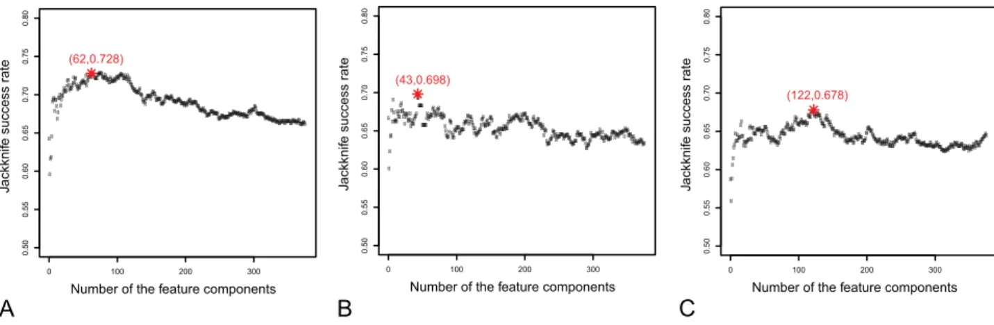
In the IFS procedure, we built 376 feature sets based on the ordered feature setS obtained in the mRMR step. Accordingly, 376 prediction models were constructed and tested as described above. Shown inFigure 2is the IFS curve for (A) all the proteins in S (cf. the 1st
equation of Eq.9), (B) only the ‘‘short’’ and ‘‘medium’’ half-life proteins (cf. the 2ndequation of Eq.9), (C) only the ‘‘long’’ and ‘‘extra-long’’ half-life proteins (cf. the 3rdequation of Eq.9). As shown inFigure 2(A), the overall accuracy reached its peak of 72.8% when the number of feature component used
was 62. The 62 feature components selected by mRMR would constitute the optimal feature set for the ‘‘short/medium’’-‘‘long/ extra-long’’ classifier. The optimal feature set for the ‘‘short’’-medium’’ classifier contained 43 feature components, with the peak success rate of 69.8%; while the optimal feature set for the ‘‘long’’-‘‘extra-long’’ classifier contained 122 feature components, with the peak success rate of 67.8%. The optimal feature components were extracted according to their impact to the success rates in predicting stability of proteins. The aforemen-tioned 62, 43, and 122 optimal feature components are provided in the Table S2 (A), (B), and (C), respectively.
Analysis of optimal feature components
To investigate what kinds of features are critical for protein stability, we extracted the optimal feature components and counted the numbers of each kind of features. Shown in Figure 3is the numbers of each kind of features in (A) the 62 feature components for the ‘‘short/medium’’-‘‘long/extra-long’’ classifier, (B) the 43 feature components for the ‘‘short’’-‘‘medium’’ classifier, and (C) the 122 feature components for the ‘‘long’’-‘‘extra-long’’ classifier, respectively. As we can see fromFigure 3, the following seven kinds of features play the major roles in affecting the protein stability: (1) KEGG enrichment scores, (2) subcellular locations, (3) polarity, (4) amino acids composition, (5) hydrophobicity, (6) secondary structure propensity, and (7) the number of protein complexes.
In a recent work Yen et al. [23] discovered that protein stability was correlated with amino acid composition. Our results have further confirmed their finding. These authors also found that the short half-life group and medium half-life group had a larger proportion of the unstable ‘‘cell cycle control’’ proteins, and that the long half-life group had a larger fraction of ‘‘mitosis’’ proteins consisting of actins, tubulins, septins, and so forth. Interestingly, our studies indicate that the metabolic stability of a protein is associated with its subcellular location, such as whether it is located in nucleus, cytoplasm, extracellular, or cell membrane, quite consistent with their findings [23] as well. Meanwhile, it was found that the enrichment of degradation, metabolism and signaling pathways could help predict protein’s metabolic stability (see Table S2), which is quite sensible as well.
bonding, hydrogen bonding, ion-pairs, and van der Waals interactions defining the shape and keeping it from falling apart [74].
A general solution for predicting the metabolic stability of proteins, even with a moderate success rate, is an extremely difficult and complicated problem. However, any progress in this regard would provide us with very useful insights for in-depth researches in protein science and developing new strategy for drug design.
The predicted metabolic stability of drug target proteins It is interesting to predict the metabolic stability of drug target proteins and compare the results with the half-life spans of the corresponding drugs. Although there were many factors that can affect the half-life of a drug, we found that the stability of its target protein is a quite important one. For demonstration, the predicted metabolic stability outcomes for some drug target proteins and the real half-life spans of their corresponding drugs are given in the Table S3, from which we found some intriguing correlations. The
half-life of drugs targeted to proteins with predicted ‘‘short or medium half-life’’ (with median of 420 minutes) was shorter than the half-life of drugs targeted to proteins with predicted ‘‘long or extra-long half-life’’ (with median of 709 minutes). The median of the half-life of drugs targeted to proteins with predicted ‘‘short half-life’’, ‘‘medium half-life’’, ‘‘long half-life’’ and ‘‘extra-long half-life’’ were 303, 510, 540 and 1080 minutes, respectively.
For instance, Dinoprostone (DrugBank accession number DB00917) is a prescription drug used, as a vaginal suppository, to prepare the cervix for labour and to induce labour. The half-life of Dinoprostone is less than 5 minutes. The predicted stability results for its target proteins PTGER1 (UniProtKB/Swiss-Prot ID P34995) and PTGER2 (UniProtKB/Swiss-Prot ID P43116) were both ‘‘short’’ half-life. Again, Clorazepate (DrugBank accession number DB00628) is for treating anxiety. It also has the function for muscle relaxant and anticonvulsant. Its half-life is about 2 days (1,440 minutes), and the predicted stability for its target proteins BZRP (UniProtKB/Swiss-Prot ID P30536) and GABRA1 (Uni-ProtKB/Swiss-Prot ID P14867) were ‘‘long’’ and ‘‘extra-long’’, Figure 2. The IFS curves of protein’s metabolic stability predictions.The IFS curves for (A) all the proteins inS(cf. Eq. 9), (B) only the ‘‘short’’ and ‘‘medium’’ half-life proteins inSshort/medium, and (C) only the ‘‘long’’ and ‘‘extra-long’’ half-life proteins inSlong/extra-long. The overall accuracy reached its peak of 72.8% when the number of feature components used for the classifier between ‘‘short/medium’’ half-life and ‘‘long/extra-long’’ half-life was 62. The corresponding accuracy peak and featured component number for the case of panel B are 69.8% and 43, while those for the case of panel C are 67.8% and 122.
doi:10.1371/journal.pone.0010972.g002
Figure 3. The numbers of each kind of features in optimal feature sets.The numbers of each kind of features for (A) the 62 feature components in the optimal ‘‘short/medium’’-‘‘long/extra-long’’ classifier, (B) the 43 feature components in the optimal ‘‘short’’-‘‘medium’’ classifier, and (C) the 122 feature components in the optimal ‘‘long’’-‘‘extra-long’’ classifier.
doi:10.1371/journal.pone.0010972.g003
Metabolic Stability Prediction
respectively, fully consistent with the sense that the more stable a protein is, the longer half-life drug is needed for effectively targeting it; and vice versa.
Discussion
We have developed a new method for predicting the metabolic stability of proteins by integrating their various biochemical and physicochemical features. It is indicated by the rigorous jackknife cross-validation test that the predictor can achieve an overall success rate of 72.8%. With the feature selection approach based on the mRMR method and IFS procedure, we found that the following seven features would play the major roles in determining the stability of proteins: KEGG enrichment scores, subcellular locations, polarity, amino acids composition, hydrophobicity, secondary structure propensity, and the number of protein complexes. These findings might provide useful information for drug development. The method presented in this paper might also become a high throughput tool for large-scale annotating the metabolic stability of proteins.
Supporting Information
Dataset S1 The sequences of benchmark dataset.
Found at: doi:10.1371/journal.pone.0010972.s001 (0.71 MB TXT)
Table S1 List of the 376 feature components.
Found at: doi:10.1371/journal.pone.0010972.s002 (0.10 MB XLS)
Table S2 The optimal feature components.
Found at: doi:10.1371/journal.pone.0010972.s003 (0.05 MB XLS)
Table S3 The predicted metabolic stability for drug target proteins.
Found at: doi:10.1371/journal.pone.0010972.s004 (0.10 MB XLS)
Acknowledgments
The authors wish to thank the two Reviewers for their constructive comments, which are very helpful for strengthening the presentation of this study.
Author Contributions
Conceived and designed the experiments: XK YXL YDC KCC. Performed the experiments: TH PW. Analyzed the data: TH ZH. Contributed reagents/materials/analysis tools: LH. Wrote the paper: TH XHS KYF.
References
1. Chou KC (1988) Review: Low-frequency collective motion in biomacromole-cules and its biological functions. Biophysical Chemistry 30: 3–48.
2. Madkan A, Blank M, Elson E, Chou KC, Geddis MS, et al. (2009) Steps to the clinic with ELF EMF. Natural Science 1: 157–165.
3. Schnell JR, Chou JJ (2008) Structure and mechanism of the M2 proton channel of influenza A virus. Nature 451: 591–595.
4. Martel P (1992) Biophysical aspects of neutron scattering from vibrational modes of proteins. Prog Biophys Mol Biol 57: 129–179.
5. Kamerzell TJ, Middaugh CR (2008) The complex inter-relationships between protein flexibility and stability. J Pharm Sci 97: 3494–3517.
6. Chou KC, Chen NY (1977) The biological functions of low-frequency phonons. Scientia Sinica 20: 447–457.
7. Chou KC (1984) The biological functions of low-frequency phonons: 4. Resonance effects and allosteric transition. Biophysical Chemistry 20: 61–71. 8. Chou KC (1987) The biological functions of low-frequency phonons: 6. A
possible dynamic mechanism of allosteric transition in antibody molecules. Biopolymers 26: 285–295.
9. Chou KC, Mao B (1988) Collective motion in DNA and its role in drug intercalation. Biopolymers 27: 1795–1815.
10. Chou KC (1989) Low-frequency resonance and cooperativity of hemoglobin. Trends in Biochemical Sciences 14: 212.
11. Chou KC, Zhang CT, Maggiora GM (1994) Solitary wave dynamics as a mechanism for explaining the internal motion during microtubule growth. Biopolymers 34: 143–153.
12. Pielak RM, Jason R, Schnell JR, Chou JJ (2009) Mechanism of drug inhibition and drug resistance of influenza A M2 channel. Proceedings of National Academy of Science, USA 106: 7379–7384.
13. Huang RB, Du QS, Wang CH, Chou KC (2008) An in-depth analysis of the biological functional studies based on the NMR M2 channel structure of influenza A virus. Biochem Biophys Res Comm 377: 1243–1247.
14. Du QS, Huang RB, Wang CH, Li XM, Chou KC (2009) Energetic analysis of the two controversial drug binding sites of the M2 proton channel in influenza A virus. Journal of Theoretical Biology 259: 159–164.
15. Wang JF, Chou KC (2009) Insight into the molecular switch mechanism of human Rab5a from molecular dynamics simulations. Biochemical and Biophysical Research Communications 390: 608–612.
16. Wang JF, Gong K, Wei DQ, Li YX, Chou KC (2009) Molecular dynamics studies on the interactions of PTP1B with inhibitors: from the first phosphate binding site to the second one. Protein Engineering Design and Selection 22: 349–355.
17. Wang JF, Yan JY, Wei DQ, Chou KC (2009) Binding of CYP2C9 with diverse drugs and its implications for metabolic mechanism. Medicinal Chemistry 5: 263–270.
18. Chou JJ, Li S, Klee CB, Bax A (2001) Solution structure of Ca2+-calmodulin reveals flexible hand-like properties of its domains. Nature Structural Biology 8: 990–997.
19. Li L, Wei DQ, Wang JF, Chou KC (2007) Computational studies of the binding mechanism of calmodulin with chrysin. Biochem Biophys Res Comm 358: 1102–1107.
20. Wei H, Wang CH, Du QS, Meng J, Chou KC (2009) Investigation into adamantane-based M2 inhibitors with FB-QSAR. Medicinal Chemistry 5: 305–317.
21. Gong K, Li L, Wang JF, Cheng F, Wei DQ, et al. (2009) Binding mechanism of H5N1 influenza virus neuraminidase with ligands and its implication for drug design. Medicinal Chemistry 5: 242–249.
22. Wang JF, Zhang CC, Chou KC, Wei DQ (2009) Review: Structure of cytochrome P450s and personalized drug. Current Medicinal Chemistry 16: 232–244.
23. Yen HC, Xu Q, Chou DM, Zhao Z, Elledge SJ (2008) Global protein stability profiling in mammalian cells. Science 322: 918–923.
24. Chou KC (2009) Pseudo amino acid composition and its applications in bioinformatics, proteomics and system biology. Current Proteomics 6: 262– 274.
25. Rice P, Longden I, Bleasby A (2000) EMBOSS: the European Molecular Biology Open Software Suite. Trends Genet 16: 276–277.
26. Chou KC (2001) Prediction of protein cellular attributes using pseudo amino acid composition. PROTEINS: Structure, Function, and Genetics (Erratum: ibid, 2001, Vol44, 60) 43: 246–255.
27. Chou KC (2005) Using amphiphilic pseudo amino acid composition to predict enzyme subfamily classes. Bioinformatics 21: 10–19.
28. Dubchak I, Muchnik I, Mayor C, Dralyuk I, Kim SH (1999) Recognition of a protein fold in the context of the SCOP classification. Proteins-Structure Function and Genetics 35: 401–407.
29. Niu B, Jin Y, Lu L, Fen K, Gu L, et al. (2009) Prediction of interaction between small molecule and enzyme using AdaBoost. Mol Divers 13: 313–320. 30. Xiao X, Chou KC (2007) Digital coding of amino acids based on hydrophobic
index. Protein & Peptide Letters 14: 871–875.
31. Zhang TL, Ding YS, Chou KC (2008) Prediction protein structural classes with pseudo amino acid composition: approximate entropy and hydrophobicity pattern. Journal of Theoretical Biology 250: 186–193.
32. Chou KC, Zhang CT (1994) Predicting protein folding types by distance functions that make allowances for amino acid interactions. Journal of Biological Chemistry 269: 22014–22020.
33. Dubchak I, Muchnik I, Mayor C, Dralyuk I, Kim SH (1999) Recognition of a protein fold in the context of the Structural Classification of Proteins (SCOP) classification. Proteins: Structure, Function, and Genetics 35: 401–407. 34. Chou KC (1995) A novel approach to predicting protein structural classes in a
(20-1)-D amino acid composition space. Proteins: Structure, Function & Genetics 21: 319–344.
36. Pollastri G, Baldi P, Fariselli P, Casadio R (2002) Prediction of coordination number and relative solvent accessibility in proteins. Proteins-Structure Function and Genetics 47: 142–53.
37. Chothia C, Finkelstein AV (1990) The classification and origins of protein folding patterns. Annu Rev Biochem 59: 1007–1039.
38. Fauchere JL, Charton M, Kier LB, Verloop A, Pliska V (1988) Amino acid side chain parameters for correlation studies in biology and pharmacology. International Journal of Peptide and Protein Research 32: 269–278. 39. Grantham R (1974) Amino acid difference formula to help explain protein
evolution. Science 185: 862–864.
40. Chou KC, Shen HB (2007) Review: Recent progresses in protein subcellular location prediction. Analytical Biochemistry 370: 1–16.
41. Chou KC, Shen HB (2008) Cell-PLoc: A package of web-servers for predicting subcellular localization of proteins in various organisms. Nature Protocols 3: 153–162.
42. The UniProt Consortium (2009) The Universal Protein Resource (UniProt) 2009. Nucl Acids Res 37: D169–174.
43. Altschul SF, Gish W, Miller W, Myers EW, Lipman DJ (1990) Basic local alignment search tool. J Mol Biol 215: 403–410.
44. Chou KC, Shen HB (2010) A new method for predicting the subcellular localization of eukaryotic proteins with both single and multiple sites: Euk-mPLoc 2.0. PLoS ONE 5: e9931.
45. Chou KC, Shen HB (2009) Review: recent advances in developing web-servers for predicting protein attributes. Natural Science 2: 63–92.
46. Biocompare website (2010) http://www.biocompare.com/Articles/FeaturedArticle/ 976/Subcellular-Targeting-Of-Proteins-And-Drugs.html.
47. Sharan R, Ulitsky I, Shamir R (2007) Network-based prediction of protein function. Mol Syst Biol 3: 88.
48. Jensen LJ, Kuhn M, Stark M, Chaffron S, Creevey C, et al. (2009) STRING 8–a global view on proteins and their functional interactions in 630 organisms. Nucleic Acids Research 37: D412–416.
49. Ruepp A, Waegele B, Lechner M, Brauner B, Dunger-Kaltenbach I, et al. (2010) CORUM: the comprehensive resource of mammalian protein complex-es–2009. Nucleic Acids Research 38: D497–501.
50. Peng H, Long F, Ding C (2005) Feature selection based on mutual information: criteria of max-dependency, max-relevance, and min-redundancy. IEEE Trans Pattern Anal Mach Intell 27: 1226–1238.
51. Chou KC, Zhang CT (1992) A correlation coefficient method to predicting protein structural classes from amino acid compositions. European Journal of Biochemistry 207: 429–433.
52. Chou KC, Zhang CT (1995) Review: Prediction of protein structural classes. Critical Reviews in Biochemistry and Molecular Biology 30: 275–349. 53. Qian Z, Cai YD, Li Y (2006) A novel computational method to predict
transcription factor DNA binding preference. Biochem Biophys Res Commun 348: 1034–1037.
54. Huang T, Cui W, Hu L, Feng K, Li YX, et al. (2009) Prediction of pharmacological and xenobiotic responses to drugs based on time course gene expression profiles. PLoS One 4: e8126.
55. Chou KC, Cai YD (2003) A new hybrid approach to predict subcellular localization of proteins by incorporating gene ontology. Biochemical and Biophysical Research Communications 311: 743–747.
56. Lin H (2008) The modified Mahalanobis discriminant for predicting outer membrane proteins by using Chou’s pseudo amino acid composition. Journal of Theoretical Biology 252: 350–356.
57. Chen C, Chen L, Zou X, Cai P (2009) Prediction of protein secondary structure content by using the concept of Chou’s pseudo amino acid composition and support vector machine. Protein & Peptide Letters 16: 27–31.
58. Ding H, Luo L, Lin H (2009) Prediction of cell wall lytic enzymes using Chou’s amphiphilic pseudo amino acid composition. Protein & Peptide Letters 16: 351–355.
59. Li FM, Li QZ (2008) Predicting protein subcellular location using Chou’s pseudo amino acid composition and improved hybrid approach. Protein & Peptide Letters 15: 612–616.
60. Lin H, Ding H, Feng-Biao Guo FB, Zhang AY, Huang J (2008) Predicting subcellular localization of mycobacterial proteins by using Chou’s pseudo amino acid composition. Protein & Peptide Letters 15: 739–744.
61. Wishart DS, Knox C, Guo AC, Cheng D, Shrivastava S, et al. (2008) DrugBank: a knowledgebase for drugs, drug actions and drug targets. Nucleic Acids Research 36: D901–906.
62. Wang J, Pielak RM, McClintock MA, Chou JJ (2009) Solution structure and functional analysis of the influenza B proton channel. Nat Struct Mol Biol 16: 1267–1271.
63. Oxenoid K, Chou JJ (2005) The structure of phospholamban pentamer reveals a channel-like architecture in membranes. Proceedings of the National Academy of Sciences of the United States of America 102: 10870–10875.
64. Cristian L, Lear JD, DeGrado WF (2003) Determination of membrane protein stability via thermodynamic coupling of folding to thiol-disulfide interchange. Protein Sci 12: 1732–1740.
65. White SH, Wimley WC (1999) Membrane protein folding and stability: physical principles. Annu Rev Biophys Biomol Struct 28: 319–365.
66. Chou KC, Carlacci L, Maggiora GM, Parodi LA, Schultz MW (1992) An energy-based approach to packing the 7-helix bundle of bacteriorhodopsin. Protein Science 1: 810–827.
67. Chou KC, Carlacci L (1991) Energetic approach to the folding of alpha/beta barrels. Proteins: Structure, Function, and Genetics 9: 280–295.
68. Lumry R (2002) Protein substructures and folded stability. Biophys Chem 101–102: 81–92.
69. Minetti CA, Remeta DP (2006) Energetics of membrane protein folding and stability. Arch Biochem Biophys 453: 32–53.
70. Shen HB, Chou KC (2009) Predicting protein fold pattern with functional domain and sequential evolution information. Journal of Theoretical Biology 256: 441–446.
71. Shen HB, Song JN, Chou KC (2009) Prediction of protein folding rates from primary sequence by fusing multiple sequential features. Journal of Biomedical Science and Engineering (JBiSE) 2: 136–143.
72. Chou KC, Shen HB (2009) FoldRate: A web-server for predicting protein folding rates from primary sequence. The Open Bioinformatics Journal 3: 31–50.
73. Gromiha MM, Selvaraj S (2004) Inter-residue interactions in protein folding and stability. Prog Biophys Mol Biol 86: 235–277.
74. Fields PA (2001) Review: Protein function at thermal extremes: balancing stability and flexibility. Comp Biochem Physiol A Mol Integr Physiol 129: 417–431.
Metabolic Stability Prediction