Technical Note
Modeling the Liquid Volume Flux in Bubbly
Jets Using a Simple Integral Approach
Iran E. Lima Neto
1Abstract:This study presents a simple model to predict the liquid volume flux induced by round bubbly jets. The model is based on the classical integral equations for bubble plumes, but also accounts for the momentum at the source by including new conditions for the initial liquid jet velocity and radius. Moreover, an exponential functional relationship is used to relate the entrainment coefficient to a densimetric Froude number. The model predicts well the experimental results available in the literature for bubbly jets. Model simulations plotted together with experimental data for both bubbly jets and bubble plumes also reveals a clear jet/plume transition, resulting in entrainment rates in the bubbly jet zone larger than those in the bubble plume zone. Finally, potential applications of the model in aeration/mixing systems are
presented.DOI:10.1061/(ASCE)HY.1943-7900.0000499.© 2012 American Society of Civil Engineers.
CE Database subject headings:Bubbles; Jets (fluid); Plumes; Two phase flow; Entrainment; Hydraulic models.
Author keywords:Bubbles; Jets; Plumes; Two phase flow; Entrainment; Integral equations.
Introduction
Bubble plumes and bubbly jets have a variety of applications in the fields of environmental, chemical, and mechanical engineering. Although bubble plumes are produced by the injection of gases in
liquids (Cederwall and Ditmars 1970;Fannelop and Sjoen 1980;
Milgram 1983; Wüest et al. 1992;Brevik and Kristiansen 2002; Lima Neto et al. 2008a,c), bubbly jets are produced by the injection
of gas-liquid mixtures (Fast and Lorenzen 1976; Sun and Faeth
1986;Iguchi et al. 1997,Lima Neto et al. 2007,2008b,d), as shown
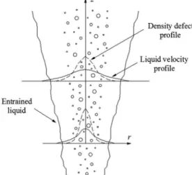
schematically in Fig.1. Bubbly jets present some advantages over
bubble plumes such as production of small bubbles without the need for porous diffusers, which are relatively expensive and sus-ceptible to clogging, and higher energy efficiency for aeration and
mixing purposes (seeLima Neto et al. 2007,2008d).
Turbulence models have been proposed to assess the liquid flow structure in bubbly jets with gas volume fractions at the nozzle lower than 10% (Sun and Faeth 1986). On the other hand, for higher gas volume fractions (up to approximately 70%), only
em-pirical relationships have been obtained (Iguchi et al. 1997;Lima
Neto et al. 2008b,d). In the present study, a simple integral ap-proach is proposed based on the classical theory for axisymmetric
bubble plumes (seeSocolofsky et al. 2002) to estimate the liquid
volume flux induced by round bubbly jets with gas volume frac-tions ranging from very low to high. This information is important to analyze the mixing patterns in aerated tanks and water bodies.
Model Formulation
The model described in the present study is based on the similarity assumptions and integral techniques for single-phase axisymmetric
jets and plumes (Morton et al. 1956;Rajaratnam 1976), but also
incorporates the effects of bubble slip velocity and bubble expan-sion (Cederwall and Ditmars 1970) and the momentum amplifica-tion factor (Milgram 1983), which are widely used for modeling the
liquid volume flux induced by bubble plumes (seeSocolofsky et al.
2002). Hence, assuming similar Gaussian distributions of axial liquid velocity and density defect at different distances from the
nozzle exit (see Fig.1), the following governing equations can be
obtained for the liquid volume conservation [Eq. (1)] and momen-tum conservation [Eq. (2)], respectively:
dðumb2Þ
dz ¼2αumb ð1Þ
dðu2 mb2Þ
dz ¼
2gQg;aHa
γπðH zÞð um
1þλ2þusÞ
ð2Þ
in whichum= the centerline liquid velocity;b= a measure of the
liquid jet radius where the velocityu=e 1¼37%of the centerline
value [i.e.,uðz;rÞ ¼umðzÞe r
2=b2
];z= the axial distance from the
nozzle exit;r= the radial distance from the jet centerline;α= the
entrainment coefficient; γ= the momentum amplification factor;
λ = the spreading ratio of the bubble core radius relative to the
liquid jet radius;us= the bubble slip velocity;Qg;a= the gas volume
flow rate at atmospheric pressure;Ha= the atmospheric pressure
head,; andH= the static pressure head at the nozzle. Note that the
effect of bubble dissolution is neglected in the preceding analysis. The reader may refer to Wüest et al. (1992) for studies on large-scale bubble plumes where the effect of bubble dissolution on the flow structure is important.
The starting conditions for the numerical integration of Eqs. (1) and (2) require the assumption of a source of buoyancy only, as in
the case of bubble plumes (Cederwall and Ditmars 1970;Milgram
1983). To solve this problem while preserving the multiphase nature of the plume, Wüest et al. (1992) defined a densimetric Froude number of 1.6 at the source. This condition has been recently validated by Socolofsky et al. (2008) and Einarsrud and Brevik (2009). However, for bubbly jets, momentum is expected to dominate the flow and an alternative approach is required. Thus, 1
Assistant Professor, Dept. of Hydraulic and Environmental Engineer-ing, Federal Univ. of Ceará, Fortaleza, Brazil. E-mail: iran@deha.ufc.br
Note. This manuscript was submitted on January 12, 2011; approved on August 1, 2011; published online on August 3, 2011. Discussion period open until July 1, 2012; separate discussions must be submitted for individual papers. This technical note is part of theJournal of Hydraulic Engineering, Vol. 138, No. 2, February 1, 2012. ©ASCE, ISSN 0733-9429/2012/2-210–215/$25.00.
rather than using the drift flux model, which considers a distribu-tion parameter and a drift velocity using some empirical reladistribu-tion-
relation-ships (seeIguchi et al. 1997), or the concept of superficial water
velocity, which neglects the effect of the gas phase on the liquid
velocity at the nozzle exit (seeLima Neto et al. 2008b,d), the
fol-lowing equation was used in the present study for the initial liquid velocity:
um;0¼
Ql;0
ð1 ε0Þðπd2=4Þ
ð3Þ
in whichd= the nozzle diameter; andε0= the gas volume fraction
at the nozzle, given by
ε0¼
Qg;0
Qg;0þQl;0
ð4Þ
in which Qg;0 and Ql;0 = the gas and liquid volume flow rates,
respectively.
Eq. (3) suggests that, for the same values ofdandQl;0, the liquid
velocityum;0increases withQg;0(orε0) because the cross-sectional
area at the nozzle exit is assumed to decrease by a factor of 1 ε0.
Instead of using corrections for the virtual origin of the liquid jet, as is often done for bubble plumes (Cederwall and Ditmars 1970;Milgram 1983), the liquid jet radius at the nozzle exit was simply taken as equal to the nozzle diameter
b0¼d ð5Þ
This assumption is supported by observations of the bubbly jets studied by Lima Neto et al. (2008b), in which extrapolation of the
linear spreading of the liquid jet resulted inb0≅d.
The momentum amplification factor (γ), spreading ratio of the
bubble core to the water jet radius (λ), and bubble slip velocity (us)
were considered constants, as is usually done in bubble plume
stud-ies (seeSocolofsky et al. 2002). Nevertheless, the values for these
parameters were obtained from investigations on bubbly jets. Thus,
an average value ofγ¼2 was obtained from the mean and
turbu-lent components of the flow induced by the bubbly jets studied by Iguchi et al. (1997). Because the momentum amplification factor
can be defined by γ¼ ðu2i þu0iu0jÞ=ðu2iÞ, in which u0i and u0j
represent the turbulent components of the flow, a value ofγ¼2
implies that a fixed proportion of 50% of the total momentum flux is attributed to turbulent transport. This value lies within the region
of 1≤γ≤3 reported by Milgram (1983) for bubble plumes.
An average value ofλ¼0:7 was obtained from Lima Neto et al.
(2008b), which is within the range of typical values of 0.4–1.0 reported by Milgram (1983) and Socolofsky et al. (2002) for bubble
plumes. An average value ofus¼0:4 m=s was also obtained from
Lima Neto et al. (2008b). This value lies within the range of
0:2–0:6 m=s reported by Milgram (1983) and Lima Neto et al.
(2008d) for bubble plumes and bubbly jets, respectively. Finally, using the Buckingham pi theorem assuming that the forces due to momentum and buoyancy dominate the flow struc-ture, the entrainment coefficient can be described by the following dimensionless relationship:
α¼fðF0Þ ð6Þ
in whichF0= a densimetric Froude number defined in this study as
Fr0¼
um;0 ffiffiffiffiffiffiffiffiffiffiffiffiffiffiffiffiffiffiffiffiffiffiffiffiffiffiffiffiffi dgðρl ρgÞ=ρl
p ð7Þ
in whichρland ρg = the liquid and gas density, respectively.
Note that Eq. (7) differs from the densimetric Froude number proposed by Wüest et al. (1992) for bubble plumes.
Therefore, Eq. (6) is the only function to be tested in order to adjust the model to experimental data. Hence, provided the form of Eq. (6) is known, Eqs. (1) and (2) can be solved numerically using a
Runge-Kutta fourth-order method to yield values ofumandbalong
the bubbly jet.
The next section shows a comparison of the model described in this study with the experimental data of Sun and Faeth (1986), Iguchi et al. (1997), and Lima Neto et al. (2008b). A sensitivity analysis was also conducted to investigate the importance of each
of the empirical parameters (γ,λ, andus) in the model results. The
present model is based on the assumption of constant values ofγ,λ,
anduswithin the bubbly jet. This condition is expected to be
at-tained for bubbly jets with nearly monodisperse bubble diameters, which occurs for nozzle Reynolds numbers larger than 8.000 (Lima Neto et al. 2008b,d). In fact, such condition generated bubbles with
relatively uniform diameters of 1–4 mm in all the aforementioned
experimental studies. The next section also shows a comparison of model simulations with experimental data from Lima Neto et al. (2008a) for bubble plumes under shallow water conditions (similar to those considered in the aforementioned bubbly jet experiments) and from Fannelop and Sjoen (1980) and Milgram and Van Houten
(1982) for bubble plumes under deeper water conditions. Table1
shows a summary of the experimental conditions for these studies on bubbly jets and bubble plumes.
Results and Discussion
The best fit of the model to the experimental data of Sun and Faeth (1986), Iguchi et al. (1997), and Lima Neto et al. (2008b) provided
values for the entrainment coefficient α varying from 0.060 to
0.095, which are higher than that for single-phase jets (0.054)
but within the typical range of values, 0.04–0.12, reported by
Milgram (1983) and Socolofsky et al. (2002) for bubble plumes. For all the tests, the densimetric Froude number was considerably
higher than 1.0 (i.e.,F0ranged from 3.2 to 46.9; see Table1),
sug-gesting that momentum, rather than buoyancy, dominated the flow
structure. Fig.2shows the fitted values ofαplotted as a function of
Fr0. The following functional relationship was obtained by
adjust-ing an exponential curve to these values:
α¼0:04þ0:06 expð 1=F0Þ4:6 ð8Þ
Fig.2shows that Eq. (8) fitted well to the data, with a correlation
coefficient C¼0:93. This suggests that F0 is an appropriate
parameter to describe the mean flow generated by bubbly jets. Fig. 1.Diagram of an axisymmetric bubble plume generated due to
gas injection in water, which is similar to that of a bubbly jet generated due to a gas-liquid injection in water
According to Eq. (8), α→0:04 as F0→0 and α→0:10 as
F0→∞. This equation is similar to that proposed by Seol et al.
(2007) for bubble plumes. Nevertheless, instead of using the
den-simetric Froude numberF0, they used a dimensionless parameter
given byus=ðB=zÞ1=3, in whichBis the kinematic buoyancy flux of
the plume. Therefore, in their case, the entrainment coefficient
varies with the axial distance from the source,z.
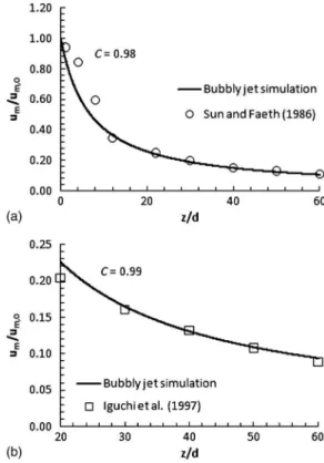
Fig. 3(a) demonstrates that model predictions fitted well
(C¼0:98) with the normalized centerline velocity (um=um;0) of
the dilute bubbly jets tested by Sun and Faeth (1986) (see Table1).
The results not only suggest that the liquid velocity at the nozzle exit is well represented by Eq. (3), but also that the combination of
Eqs. (1)–(3), (5), and (8) describes well the velocity decay,
espe-cially for the range of normalized distance from the source (z=d)
between 10 and 60. Fig. 3(b) shows the fit of the model to the
values ofum=um;0for the bubbly jets investigated by Iguchi et al.
(1997), which had higher gas volume fractions than those studied by Sun and Faeth (1986). The results show that the model predicts
well (C¼0:99) the velocity decay for the range ofz=dbetween 20
and 60. Measurements forz=d<20 (where the gas volume fraction
was higher) are not shown in Fig.3(b)because of their inaccuracy,
as reported by the authors. Fig.4also confirms a good fit of the
model (C≥0:98) to the radial distributions of liquid velocity
[given by uðz;rÞ ¼umðzÞe r
2=b2
] for the bubbly jets studied by Lima Neto et al. (2008b), which included different nozzle diame-ters. The model also fitted well with the other data sets not shown here, resulting in correlation coefficients higher than 0.97 and stan-dard deviations between model predictions and experiments of up to 17%. This gives credence to the considerations employed in the formulations.
The initial liquid velocitiesum;0 estimated from Eq. (3) ranged
from 4.1 to 18.4 times larger than those obtained by using the methodology of Wüest et al. (1992) for bubble plumes, i.e., a
densimetric Froude number of 1.6 at the source. Therefore, Eq. (3) is more suitable to predict this parameter in bubbly jets than their methodology. The initial velocities were also larger than those ob-tained using the drift flux model adopted by Iguchi et al. (1997) (from 1.02 to 2.13 times higher) and the superficial water velocity
concept adopted by Lima Neto et al. (2008b,d) (from 1.06 to 3.5
times higher). Because of the lack of data near the nozzle exit for gas volume fractions higher than those of Sun and Faeth (1986)
(i.e.,ε0<10%, resulting in similar initial velocities for the three
models), it cannot be affirmed that one model is superior to the
other to estimateum;0. However, values ofb0much larger than d
had to be used to fit the experimental data applying the drift flux model or the superficial water velocity concept, especially for
larger values ofε0. This suggests that Eq. (3) is also more suitable
to predictum;0using the present study’s integral approach, as in this
case the simple relationship b0¼d, verified experimentally by
Lima Neto et al. (2008b), was applicable.
A sensitivity analysis was conducted to assess the relevance of
each of the empirical parameters (γ,λ, andus) on the model results.
Table 1.Experimental Conditions for Bubbly Jets and Bubble Plumes
Authors Flow type
Static pressure
head (m) d(mm)
Gas volume flow rate (l=min)
Liquid volume flow rate (l=min)
Gas volume fraction (%)
Froude number
Sun and Faeth (1986) Bubbly jet 0.91 5.08 0.05–0.2 2 2–10 7.4–8
Iguchi et al. (1997) Bubbly jet 0.4 5 0.6–2.4 2.5–5 11–49 12–28.3 Lima Neto et al. (2008b) Bubbly jet 0.76 4–13.5 0.4–5 2–7 5–71 3.2–46.9 Milgram and Van Houten (1982) Bubble plume 3.66 16 9.4–103.5 0 100 1.6a
Fannelop and Sjoen (1980) Bubble plume 10 100 152.5–610 0 100 1.6a
Lima Neto et al. (2008a) Bubble plume 0.76 3 2–3 0 100 1.6a
a
Froude number at the source, as suggested by Wüest et al. (1992).
Fig. 2. Entrainment coefficient versus densimetric Froude number, indicating a fitted exponential curve
Fig. 3.Comparison of model predictions of normalized centerline ve-locity decay with experimental data of Sun and Faeth (1986) and Iguchi et al. (1997): (a)d¼5:08 mm,H¼0:91 m,Qg;0¼0:1 l=min,Ql;0¼ 2:0 l=min, ε0¼5%, and F0¼7:6; (b) d¼5 mm, H¼0:4 m, Qg;0¼2:4 l=min,Ql;0¼2:5 l=min,ε0¼49%, andF0¼18:9
The values ofγvaried from 1 to 3 (as reported byMilgram 1983),
λ varied from 0.4 to 1.0 (as reported by Milgram 1983 and
Socolofsky et al. 2002), andusvaried from 0.2 to 0:6 m=s (as
re-ported byMilgram 1983and Lima Neto et al. 2008b). The most
sensitive parameter was the momentum amplification factor (γ).
However, because the maximum variation of um and b from the
model calculations using the standard values (γ¼2,λ¼0:7, and
us¼0:4 m=s) was lower than 20%, it can be inferred that the
model is not highly sensitive to the range of parameters and exper-imental conditions evaluated here.
Bubbly jets are expected to be controlled by the kinematic fluxes of momentum and buoyancy at the source, which can be
expressed byM0¼Ql;0um;0 and B0¼Qg;0gðρl ρgÞ=ρl,
respec-tively. Thus, a length scale L can be defined as L¼M30=4=B
1=2 0
(seeLima Neto et al. 2008d). Similarly to single-phase buoyant
jets (seePapanicolaou and List 1988),Ldescribes the relative
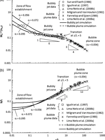
im-portance of momentum and buoyancy fluxes. Figs.5(a)and 5(b)
show, respectively, the normalized centerline velocity inverse
M10=2=ðumzÞand the normalized liquid jet radiusb=Las a function
of a normalized distance from the source,z=L, both obtained from
experimental data for bubbly jets and bubble plumes (see Table1).
The figures indicate the behavior of the curves in three regions: zone of flow establishment, bubbly jet zone, and bubble plume zone. The zone of flow establishment was defined here as the
axial distance from the nozzle exit up toz¼0:1L, which coincided
with the classical limit ofz¼5d(seeRajaratnam 1976) when
con-sidering the experiments of Sun and Faeth (1986), the only set of data obtained from measurements taken within this region. The
bubbly jet zone was defined as the region beyondz¼0:1Lwhere
M10=2=ðumzÞdecreased withz=Lfollowing a slope of 1=6, while
b=Lincreased withz=Lfollowing a slope of 1=8. A change in these
slopes at approximatelyz=L¼5 clearly shows a transition from the
momentum-dominated region (bubbly jet zone) to the buoyancy-dominated region (bubble plume zone). Therefore, the bubble
plume zone was defined as the region beyond z¼5L where
M10=2=ðumzÞdecreased withz=Lfollowing a slope of 3=4, while
b=Lincreased withz=Lfollowing a slope of 1=12. It is interesting
to observe that similar transitions and slopes have been obtained for single-phase buoyant jets, as reported by Papanicolaou and List (1988). The preceding trends can be confirmed by the bubbly jet
and bubble plume simulations depicted in Figs.5(a)and5(b). The
bubbly jet simulations were performed forz≤5Lusing the present
model, whereas the bubble plume simulations were performed for
z>5Lby including the entrainment coefficient relationship of Seol
et al. (2007) into the present model. In the bubbly jet case, three
values for the entrainment coefficientα¼0:056, 0.072, and 0.095
were used, which were within the range ofαshown in Fig.2. The
intermediate value of 0.072 was selected because it provided the best fit of the model to the data at the zone of flow establishment.
The results shown in Figs.5(a)and5(b)illustrate the sensitivity of
the model with respect toα, specially forz=L<1. In the bubble
plume case, an average value ofα¼0:054 was used to extrapolate
the intermediate condition for the bubbly jet simulation (i.e.,α¼
0:072). This implies that closer to the source (i.e., in the bubbly jet
zone) the flow is expected to have higher entrainment rates than Fig. 4.Comparison of model predictions of normalized radial
distri-butions of liquid velocity atz¼0:43 m with experimental data of Lima Neto et al. (2008b): (a)d¼9 mm, Qg;0¼2 l=min,Ql;0¼5 l=min, ε¼29%, and F¼6:18; (b) d¼13:5 mm, Qg;0¼3 l=min, Ql;0¼ 7 l=min,ε¼30%, and F¼3:2
Fig. 5.Model simulations plotted together with experimental data in a dimensionless framework: (a) centerline liquid velocity inverse as a function of distance from the source; (b) liquid jet radius as a function of distance from the source; different regions of the flow, including their curve slopes and a transition from a bubbly jet zone to a bubble plume zone, are also indicated
away from the source (i.e., in the bubble plume zone). This result
seems reasonable, as a decay ofαwithzhas been verified
exper-imentally by Seol et al. (2007) for bubble plumes.
Application
The integral approach proposed in the present study can be applied
to estimate the liquid volume flux (Ql¼πumb2) induced by round
bubbly jets in aeration/mixing systems. Consider for example a
nozzle with d¼38 mm discharging wastewater (Ql;0¼2:3 l=s)
from the bottom of a tank with water depth H¼5 m, which
results in a single-phase jet with a volume flux atz¼4:17 m of
Ql¼100 l=s [assuming an initial surface jet thickness ofH=6¼
0:83 m, as suggested by Lima Neto et al. (2008a,c), and using the
integral model for single-phase jets, as described by Rajaratnam (1976)]. Hence, if a higher liquid volume flux is required to provide additional mixing, aeration, and/or prevent suspended solids deposition, an air line can be connected to the wastewater line to produce bubbly jets. This solution has the advantage of using the existing wastewater discharge system instead of installing new
bub-ble plume diffusers (seeLima Neto et al. 2007). Therefore, the
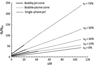
in-tegral approach proposed in this study can be used to predict the
increase in the normalized liquid volume flux (Ql=Ql;0) with the
normalized distance from the source (z=d) for different gas volume
fractionsε0, as shown in Fig.6. It can be seen that liquid volume
fluxes atz¼4:17 m ranging from approximately 1.3 to 5.5 times
higher than that for the single-phase jet can be obtained by varying
ε0 from 10% to 70% (i.e., keepingQl;0¼2:3 l=s and increasing
Qg;0 from 0.25 to 5:33 l=s). Fig. 6 also confirms that the larger
the values of ε0, the shorter the bubbly jet zone as compared to
the bubble plume zone. A similar analysis can also be performed for the cases of aerated ponds, reservoirs, and other water bodies. However, caution should be taken when applying the present model
for much deeper water conditions (H∼50 m), because in such cases
bubble dissolution may play an important role in the flow dynam-ics, as pointed out by Wüest et al. (1992) and Socolofsky et al. (2002). Additional limitations include gas volume fractions of up to approximately 70% and nozzle Reynolds numbers larger than 8.000, which were conditions imposed from the experiments used
to validate the model (seeLima Neto et al. 2008b,d).
Conclusions
In this study, a simple integral approach is proposed to estimate the liquid volume flux in axisymmetric bubbly jets. The model is sim-ilar to the classical theory for bubble plumes, but also accounts for the effect of momentum at the nozzle, including new conditions for the initial velocity and radius of the liquid jet. Using a simple ex-ponential equation to relate the entrainment coefficient to a densi-metric Froude number, a good fit of the model to the experimental data available for bubbly jets was obtained. Experimental data and model predictions also including a bubble plume regimen were plotted in a dimensionless framework using appropriate scales based on the kinematic fluxes of momentum and buoyancy at the source. This revealed three regions: zone of flow establishment, momentum-dominated zone (or bubbly jet zone), and buoyancy-dominated zone (or bubble plume zone), similar to single-phase buoyant jets. A clear transition between these regions was obtained, such that model simulations could be performed considering a bub-bly jet zone and a bubble plume zone separately. Model results yielded larger entrainment rates in the bubbly jet zone than in the bubble plume zone, which is consistent with recent experimen-tal results available in the literature. Finally, an application of the model for analysis of the circulation flow patterns in aerated tanks and water bodies is presented.
Acknowledgments
The author thanks the anonymous reviewers for their valuable comments and suggestions.
References
Brevik, I., and Kristiansen, Ø. (2002).“The flow in and around air-bubble plumes.”Int. J. Multiphase Flow, 28(4), 617–634.
Cederwall, K., and Ditmars, J. D. (1970).“Analysis of air-bubble plumes.” Rep. No. KH-R-24, W. M. Keck Laboratory of Hydraulics and Water Resources, Division of Engineering and Applied Science, CA Institute of Technology, Pasadena, CA.
Einarsrud, K. E., and Brevik, I. (2009).“Kinetic energy approach to dis-solving axisymmetric multiphase plumes.”J. Hydraul. Eng., 135(12), 1041–1051.
Fannelop, T. K., and Sjoen, K. (1980). “Hydrodynamics of underwater blowouts.” AIAA 8th Aerospace Sciences Meeting, Pasadena, CA, 80–0219.
Fast, A. W., and Lorenzen, M. W. (1976).“Synoptic survey of hypolimnetic aeration.”J. Environ. Eng. Div., 102(6), 1161–1173.
Iguchi, M., Okita, K., Nakatani, T., and Kasai, N. (1997). “Structure of turbulent round bubbling jet generated by premixed gas and liquid injection.”Int. J. Multiphase Flow, 23(2), 249–262.
Lima Neto, I. E., Zhu, D. Z., and Rajaratnam, N. (2008a).“Air injec-tion in water with different nozzles.” J. Environ. Eng., 134(4), 283–294.
Lima Neto, I. E., Zhu, D. Z., and Rajaratnam, N. (2008b).“Bubbly jets in stagnant water.”Int. J. Multiphase Flow, 34(12), 1130–1141. Lima Neto, I. E., Zhu, D. Z., and Rajaratnam, N. (2008c).“Effect of tank
size and geometry on the flow induced by circular bubble plumes and water jets.”J. Hydraul. Eng., 134(6), 833–842.
Lima Neto, I. E., Zhu, D. Z., and Rajaratnam, N. (2008d). “Horizontal injection of gas-liquid mixtures in a water tank.” J. Hydraul. Eng., 134(12), 1722–1731.
Lima Neto, I. E., Zhu, D. Z., Rajaratnam, N., Yu, T., Spafford, M., and McEachern, P. (2007).“Dissolved oxygen downstream of an effluent outfall in an ice-covered river: Natural and artificial aeration.”J. Envi-ron. Eng., 133(11), 1051–1060.
Milgram, H. J. (1983). “Mean flow in round bubble plumes.”J. Fluid Mech., 133, 345–376.
Fig. 6.Model simulations of normalized liquid volume flux as a func-tion of normalized distance from the source for a single-phase jet (ε0¼0%) and bubbly jets with different gas volume fractions (ε0¼10 to 70%); a liquid flow rate at the nozzle ofQl;0¼2:3 l=s is considered for all the cases
Milgram, H. J., and Van Houten, R. J. (1982).“Plumes from subsea well blowouts.” Proc., 3rd Int. Conf., Behavior of Offshore Structures (BOSS), Vol. I, MIT, Cambridge, MA, 659–684.
Morton, B. R., Taylor, G. I., and Turner, J. S. (1956).“Turbulent gravita-tional convection from maintained and instantaneous sources.”Proc. R. Soc. London, Ser. A, 234(1196), 1–23.
Papanicolaou, P., and List, E. J. (1988).“Investigations of round vertical turbulent buoyant jets.”J. Fluid Mech., 195, 341–391.
Rajaratnam, N. (1976). Turbulent jets, Elsevier Scientific, Amsterdam, Netherlands.
Seol, D. G., Bhaumik, T., Bergmann, C., and Socolofsky, S. A. (2007). “Particle image velocimetry measurements of the mean flow characteristics in a bubble plume.” J. Eng. Mech., 133(6), 665–676.
Socolofsky, S. A., Bhaumik, T., and Seol, D. G. (2008). “ Double-plume integral models for near-field mixing in multiphase Double-plumes.”
J. Hydraul. Eng., 134(6), 772–783.
Socolofsky, S. A., Crounse, B. C., and Adams, E. E. (2002). “ Multi-phase plumes in uniform, stratified, and flowing environments.” Envi-ronmental fluid mechanics theories and applications, H. Shen, A. Cheng, K.-H. Wang, M. H. Teng and C. Liu, eds., ASCE, Reston, VA, 85–125.
Sun, T. Y., and Faeth, G. M. (1986).“Structure of turbulent bubbly jets—I. Methods and centerline properties.”Int. J. Multiphase Flow, 12(1), 99–114.
Wüest, A., Brooks, N. H., and Imboden, D. M. (1992).“Bubble plume modelling for lake restoration.” Water Resour. Res., 28(12), 3235–3250.