ISSN 0104-6632 Printed in Brazil
www.abeq.org.br/bjche
Vol. 32, No. 02, pp. 475 - 487, April - June, 2015 dx.doi.org/10.1590/0104-6632.20150322s00003371
*To whom correspondence should be addressed
Brazilian Journal
of Chemical
Engineering
SELF-SIMILARITY OF VERTICAL BUBBLY JETS
I. E. Lima Neto
Assistant Professor, Dept. of Hydraulic and Environmental Engineering, Federal University of Ceará, Fortaleza - CE, Brazil.
E-mail: [email protected]
(Submitted: March 18, 2014 ; Revised: October 2, 2014 ; Accepted: October 14, 2014)
Abstract - An integral model for vertical bubbly jets with nearly monodisperse bubble sizes is presented. The model is based on the Gaussian type self-similarity of mean liquid velocity, bubble velocity and void fraction, as well as on functional relationships for initial liquid jet velocity and radius, bubble diameter and relative velocity. Adjusting the model to experimental data available in the literature for a wide range of densimetric Froude numbers provide constant values for the entrainment coefficient, momentum amplification factor, and spreading ratio of the bubble core for different flow conditions. Consistency and sensitivity of key model parameters are also verified. Overall, the deviations between model predictions and axial/radial profiles of mean liquid velocity, bubble velocity and void fraction are lower than about 20%, which suggests that bubbly jets tend to behave as self-preserving shear flows, similarly to single-phase jets and plumes. Furthermore, model simulations indicate a behavior similar to those of single-phase buoyant jets and slurry jets, but some differences with respect to confined bubbly jets are highlighted. This article provides not only a contribution to the problem of self-similarity in two-phase jets, but also a comprehensive model that can be used for analysis of artificial aeration/mixing systems involving bubbly jets.
Keywords: Bubbles; Gaussian profiles; Integral model; Jets; Self-preservation.
INTRODUCTION
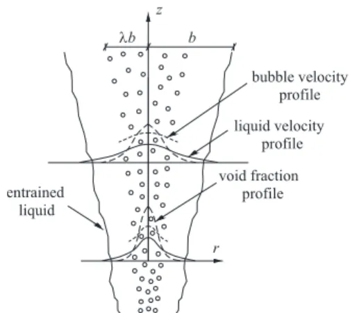
Bubbly jets are produced by the injection of gas-liquid mixtures into gas-liquids, as shown schematically in Figure 1. Such two-phase flows are encountered in diverse engineering applications, including gas-liquid mass transfer, heat transfer and turbulent mixing in reactors, tanks and water bodies (Sun and Faeth, 1986a; Iguchi et al., 1997; Morchain et al., 2000; Mueller et al., 2002; Lima Neto et al., 2007; Suñol and González-Cinca, 2010; Norman and Revankar, 2011; Lima Neto, 2012b; Zhang and Zhu, 2013).
A number of experimental studies have been con-ducted to investigate the flow structure of bubbly jets. The first comprehensive investigation on this subject was reported by Sun and Faeth (1986a,b), who studied vertical bubbly jets with gas volume fractions at the nozzle of up to about 9% and found that mean and turbulent properties of the flow were
476 I. E. Lima Neto
bubbles, and suggested that a nozzle Reynolds num-ber larger than 8.000 is needed to produce relatively small bubbles with approximately uniform diame-ters. Note that while the studies of Sun and Faeth (1986a,b), Kumar et al. (1989) and Iguchi et al. (1997) were carried out in confined setups (as dis-cussed by Lima Neto et al., 2008c), the study of Lima Neto et al. (2008b) was performed in a large tank, in which the bubbly jets were located far enough from the walls so that they could behave as free jets. Other experimental studies on bubbly jets including the effects of angled-injections, crossflow, collision or periodical excitation of such two-phase flows have also been performed (Varley, 1995; Milenkovic et al., 2007; Lima Neto et al., 2008d; Suñol and González-Cinca, 2010; Zhang and Zhu, 2013). It is interesting to mention that Gaussian pro-files of void fraction were still observed in experi-ments of bubbly jets in crossflow, as pointed out by Zhang and Zhu (2013). Additionally, they found that a nozzle Reynolds number larger than 8.000 is in-deed necessary to produce nearly uniform bubble size distributions, as suggested by Lima Neto et al. (2008b). Lima Neto et al. (2008d) obtained the same result for horizontally-injected bubbly jets.
entrained liquid
liquid velocity profile void fraction profile
z
r
bubble velocity profile
λb b
Figure 1: Schematic of a vertical bubbly jet, assum-ing Gaussian type self-similarity of liquid velocity, bubble velocity and void fraction along the axial direction.
Contrasting with the numerous experimental stud-ies on bubbly jets, theoretical studstud-ies on this topic are scarce. Sun and Faeth (1986a,b) predicted the two-phase flow structure of their dilute vertical bub-bly jets (with gas volume fractions at the nozzle of up to about 9%) using k-ε type turbulence models. Reasonably good predictions compared to their ex-perimental data were obtained when bubble slip ve-locity and bubble-turbulence interactions were
con-sidered using random-walk methods. More recently, Lima Neto (2012b) proposed a simple model to pre-dict the mean liquid flow structure of vertical bubbly jets with gas volume fractions of up to 71%, which is based on the Gaussian type self-similarity assump-tion and integral techniques for single-phase jets and plumes (Morton et al., 1956), but also incorporates the effects of bubble slip velocity and bubble expan-sion (Cederwall and Ditmars, 1970) and the factor of momentum amplification due to turbulence (Milgram, 1983). Using appropriate conditions for the initial liquid jet velocity and radius and a functional re-lationship to relate the entrainment coefficient to a densimetric Froude number, Lima Neto’s model predicted the liquid velocities induced by bubbly jets. Model simulations plotted together with experi-mental data for both bubbly jets and bubble plumes also revealed a clear jet/plume transition, suggesting that model simulations could be performed by con-sidering a bubbly jet zone followed by a bubble plume zone. Nevertheless, gas-phase characteristics (bubble velocity and void fraction) were not investi-gated, since integral models are not expected to ac-curately predict the net buoyant force acting on simi-lar bubbly flows (i.e., bubble plumes), as pointed out by Socolofsky et al. (2002) and Socolofsky et al. (2008). In fact, even for single-phase jets and plumes, complete self-similarity remains a debatable issue (Wygnanski and Fiedler, 1969; Carazzo et al., 2006; Zhang et al., 2011). Other theoretical studies on bubbly jets including the effects of angled-injec-tions, crossflow and stratification have also been per-formed (Morchain et al., 2000; Norman and Revankar, 2011).
Brazilian Journal of Chemical Engineering Vol. 32, No. 02, pp. 475 - 487, April - June, 2015 MODEL FORMULATION,
PARAMETERIZATION AND OPTIMIZATION
The model proposed in this study assumes that vertical bubbly jets exhibit self-similarity, as usually done for single-phase jets and plumes (Zhang et al., 2011). Thus, in order to simplify the relationships for the variation of the two-phase flow properties of the bubbly jets along the axial direction z, the distribu-tions of liquid velocity (u), bubble velocity (w) and void fraction (C) along the radial direction r are as-sumed to be Gaussian (see Figure 1):
( )
2 2, = c( ) −r b
u r z u z e (1)
( )
2 2, = c( ) −r b + s
w r z u z e u (2)
( )
2 ( )2, = c( ) −r b
C r z C z e λ (3)
in which uc, wc and Cc are respectively the liquid
velocity, bubble velocity, and void fraction at the bubbly jet centerline, b is a measure of the liquid jet radius where the liquid velocity u is e-1 = 37% of the centerline value, us is the bubble slip velocity
(as-sumed constant for monodisperse bubble diameters), and λ is the spreading ratio of the bubble core radius relative to the liquid jet radius.
Because the distributions of u, w and C are de-scribed by Eqs. (1) - (3), state variables can be inte-grated over the radial direction r to obtain integral fluxes of volume, momentum and buoyancy that are functions only of the axial direction z, reducing the problem to one dimension. Hence, the following equations are obtained by invoking conservation of volume (using the entrainment hypothesis closure), conservation of momentum (equating the spatial rate of change of momentum flux to the total buoyancy force per unit height of the jet), and conservation of the dispersed phase buoyancy (using the ideal gas law together with adiabatic expansion):
( )
2 2 =c c
d
u b bu
dz π π α (4)
(
)
2 2 2 2
2
⎛ ⎞ = −
⎜ ⎟
⎝ l c ⎠ c l g
d
u b b C g
dz γ ρ π πλ ρ ρ (5)
(
)
(
)
2 2 2 1 ⎡ − ⎛ + ⎞⎤ ⎜ ⎟ ⎢ ⎝ + ⎠⎥ ⎣ ⎦ ⎡ − ⎤ ⎢ ⎥ = − ⎢ ⎥ ⎣ ⎦ cc l g s
l g ga a
d u
b C g u
dz
Q H d
dz H z
πλ ρ ρ
λ
ρ ρ (6)
in which α is the entrainment coefficient, γ is the factor of momentum amplification due to turbulence,
ρl and ρg are the liquid and gas density, respectively,
Qga is the gas volume flow rate at atmospheric
pres-sure, Ha is the atmospheric pressure head, and His
the static pressure head at the nozzle. Eq. (4) is the same proposed by Lima Neto (2012b) to evaluate the axial variation of the liquid volume flux induced by bubbly jets. Eq. (5) is modified from the correspond-ing equation of Lima Neto (2012b) in order to ex-press the axial variation of the momentum flux in terms of the centerline void fraction Cc. Eq. (6) is
included here to allow the evaluation of the buoy-ancy flux (or the centerline void fraction Cc) along
the axial direction. Therefore, the integral model described herein is based on a system of three con-servation equations in the form of ordinary differen-tial equations, in which the variables to be solved for are uc, b, and Cc. Observe that gas-liquid mass
trans-fer is neglected in the present study, but may be in-cluded for deep water applications (see Wüest et al., 1992). Moreover, for such conditions, a jet/plume transition may also exist, so that the model must be modified in order to incorporate this effect (see Lima Neto, 2012b).
The bubble slip velocity us can be obtained using
the following relationship, which was adjusted herein with the experimental data of Lima Neto et al. (2008a,b,d) for mean bubble diameters db ranging
from about 1 to 4 mm:
4.3 34.6
= +
s b
u d (7)
where us is given in cm/s and db is given in mm. Eq.
(7) predicts the experimental data of Lima Neto et al. (2008a,b,d) with deviations of up to about 25%. Therefore, this equation will be used in the present model, rather than using an average value of us for all
simulations (Lima Neto, 2012b). Observe that Eq. (7) provides bubble slip velocities ranging from about 1.3 to 2.1 times higher than the corresponding terminal velocities reported by Clift et al. (1978) for individual bubbles.
On the other hand, the mean bubble diameter db
can be obtained by adjusting the following relation-ship to the experimental data of Sun and Faeth (1986a,b), Iguchi et al. (1997), Lima Neto et al. (2008b,d) and Zhang and Zhu (2013):
4
0.3 10 0.1 Re ⎛ ⎞ = × ⎜ ⎟+ ⎝ ⎠ b o d C
δ (8)
478 I. E. Lima Neto
by =
(
2)
1 5 goQ g
δ , while Co is the gas volume
frac-tion at the nozzle and Re is the Reynolds number based on the superficial liquid velocity:
= + go o go lo Q C
Q Q (9)
4 Re= lo
l
Q d
π ν (10)
where Qgo and Qlo are the gas and liquid volume flow
rates at the nozzle, respectively, d is the nozzle di-ameter and νl is the liquid kinematic viscosity.
Eq. (8) predicts the experimental data of Sun and Faeth (1986a,b), Iguchi et al. (1997), Lima Neto et al. (2008b,d) and Zhang and Zhu (2013) with devia-tions of up to about 20% and thus will be used in the present model. Furthermore, this equation can also be used in bubbly jet studies considering gas-liquid mass transfer effects.
It is relevant to stress that the above relationships [Eqs. (7) and (8)] were obtained for nearly uniform bubble size distributions. As already mentioned, this condition was attained for Re > 8.000 (see Lima Neto et al., 2008b,d; Zhang and Zhu, 2013). Note that the data of Kumar et al. (1989) was not consid-ered here because most of their tests were conducted for Re < 8.000 and they had to use a screen assembly before the nozzle to break large bubbles into smaller bubbles and produce approximately uniform sizes.
Assuming that uniform bubble sizes result from the occurrence of the so-called bubbly flow regime at the source, the drift flux model of Zuber and Findlay (1965) seems appropriate to evaluate the liquid ve-locity at the nozzle exit, as already suggested by Iguchi et al. (1997):
(
)
(
)
1 1 − − = −o T o G
o
o
C V C V
u
C
θ
(11)
where θ is a distribution parameter, VT is the average
volumetric flux density, and VG is the drift velocity,
which are given by the following expressions:
1 2
1.2 0.2⎛ ⎞
= − ⎜ ⎟
⎝ ⎠
g
l
ρ
θ ρ (12)
2 4 +
= lo go
T
Q Q
V
d
π (13)
(
)
1 42 2⎡⎢ − ⎤⎥ = ⎢ ⎥ ⎣ ⎦ l g G l g
V σ ρ ρ
ρ (14)
in which σ is the liquid surface tension.
Therefore, Eq. (11) will be used herein to evalu-ate the liquid velocity at the nozzle exit. For the sake of simplicity, the model of Lima Neto (2012b) used Eq. (13) to estimate this velocity, while the experi-mental study of Lima Neto et al. (2008b) considered the superficial liquid velocity [obtained by setting Qgo to zero in Eq. (13)] to fit their empirical
correla-tions. Such alternative approaches will also be tested in the present study.
Instead of using corrections for the virtual origin of the flow, as often done for bubble plumes (Lima Neto, 2012a), the liquid jet radius at the nozzle exit was simply taken as equal to the nozzle diameter:
= o
b d (15)
This assumption is supported by experimental ob-servations of Lima Neto et al. (2008b) and was used by Lima Neto (2012b) to predict the liquid volume flux induced by bubbly jets.
Finally, the three remaining parameters to be de-termined from the governing equations [Eqs. (4) - (6)] are the spreading ratio of the bubble core λ, entrainment coefficient α, and momentum amplifica-tion factor γ. Since the model described here assumes that bubbly jets exhibit self-similarity, the above-mentioned parameters must be considered constants. Hence, provided these constants are known, the sys-tem of governing equations can be solved simultane-ously using an appropriate numerical scheme (4th order Runge–Kutta) to yield values of uc, b and Cc
along the axial direction z. Furthermore, the distribu-tions of liquid velocity u, bubble velocity w and void fraction C along the radial direction r can be ob-tained from Eqs. (1) - (3). Note that, for all the nu-merical simulations, small values of dz of up to about 1% of the water depth H were used. These values were fine enough to yield accurate results, with de-viations of less than 1% from those obtained with finer step sizes.
Brazilian Journal of Chemical Engineering Vol. 32, No. 02, pp. 475 - 487, April - June, 2015
number to evaluate α for each flow condition. In the present study, in order to reach a complete self-similarity of the flow, the parameters λ, α, and γ will be fitted to experimental data of Lima Neto et al. (2008b), which included tests with densimetric Froude numbers at the nozzle exit ranging from 5.4 to 47.5 (see Expt. 1-15 in Table 1). Note that the densimetric Froude number used in this study differs from that of Lima Neto (2012b) and is given by the following expression:
(
)
=
− o
l m l
u Fr
dg ρ ρ ρ (16)
where the mixture density at the nozzle ρm is de-fined as ρm=⎡⎣
(
1−Co)
ρl+Coρg⎦⎤. Since Eq. (16) accounts for both momentum and buoyancy forces at the source, including the effect of ρm for each flow condition, it is more appropriate than that of Lima Neto (2012b) for comparison of the behavior of bub-bly jets with single-phase buoyant jets, which will be done in the next section. For the single-phase case,m
ρ is simply taken as the liquid jet density at the source.
Therefore, the constant values for the spreading ratio of the bubble core λ, entrainment coefficient α, and momentum amplification factor γ were opti-mized by solving the following objective function used to minimize the deviations between the present
integral model predictions and the experimental data of Lima Neto et al. (2008b):
Minimize:
(
')
21 1
= =
−
∑∑
n mi i
i j
χ χ (17)
by varying α, γ and λ, subject to the following constraints within the ranges reported by Milgram (1983), Socolofsky et al. (2002), Lima Neto et al. (2008a,b,c,d) and Lima Neto (2012a,b) for bubble plumes and bubbly jets:
0.040 ≤ ≤a 0.120
1.0 ≤ ≤g 3.0
0.4 ≤ ≤l 1.0
In Eq. (17), n and m correspond respectively to the number of flow conditions (n = 15) studied by Lima Neto et al. (2008b) (see Table 1) and the num-ber of data points (m = 8) for each experimental con-dition. The parameters χi and
'
i
χ represent respec-tively the model predictions and experimental data of mean liquid velocity (4 data points) and void fraction (4 data points), for each experimental condition (total of 15 experiments = 120 data points). The objective function was used to minimize the sum of the devia-tions between χi and χi', i.e., the sum of 120 devia-tions between model predicdevia-tions and experiments.
Table 1: Experimental conditions of vertical bubbly jets used for comparison with the present model simulations.
Expt. Reference H
(m)
L (m)*
d (mm)
Qgo (l/min)
Qlo (l/min)
Co (%)
Re Fr
1 13.5 3.00 7.00 30.0 11003 5.4
2 9.0 5.00 3.50 58.8 8252 7.1
3 9.0 2.00 5.00 28.6 11789 10.7
4 6.0 3.00 3.00 50.0 10610 16.6
5 6.0 5.00 3.00 62.5 10610 16.7
6 6.0 5.00 4.00 55.6 14147 22.3
7 6.0 5.00 5.00 50.0 17684 27.7
8 Lima Neto et al. (2008b) 0.8 1.2 6.0 4.00 5.00 44.4 17684 27.8
9 9.0 0.40 7.00 5.4 16505 27.8
10 6.0 3.00 5.00 37.5 17684 28.1
11 4.0 5.00 2.00 71.4 10610 28.7
12 6.0 2.00 5.00 28.6 17684 29.4
13 4.0 1.00 2.00 33.3 10610 31.5
14 6.0 1.00 5.00 16.7 17684 34.4
15 6.0 0.40 5.00 7.4 17684 47.5
16 5.1 0.20 2.00 9.1 8355 26.4
17 Sun and Faeth (1986a,b) 0.9 0.4 5.1 0.10 2.00 4.8 8355 34.8
18 5.1 0.05 2.00 2.4 8355 47.4
19 5.0 2.40 2.50 49.0 10610 22.1
20 Iguchi et al. (1997) 0.4 0.2 5.0 1.20 2.50 32.4 10610 22.8
21 5.0 0.60 5.00 10.7 21221 63.7
480 I. E. Lima Neto
Observe that this data only included values of mean liquid velocity and void fraction, since bubble velocity can be obtained directly from liquid velocity by using Eqs. (2) and (7).
The next section shows model predictions of the mean liquid velocity, bubble velocity and void frac-tion using the optimized values of α, γ and λ. The impact of different combinations of α, γ, and λ, as well as of different approaches for evaluation of the liquid velocity at the nozzle exit and the bubble rela-tive velocity are also investigated. Model predictions are compared not only with the data of liquid ve-locity and void fraction used to obtain the fitting parameters (α, γ and λ), but also with independent data of Lima Neto et al. (2008b) for bubble velocity, Iguchi et al. (1997) for liquid velocity, and Sun and Faeth (1986a,b) for both liquid and bubble velocity. Again, the experimental results of Kumar et al. (1989) were not used for comparison as their study focused on the turbulence near the nozzle exit of very confined bubbly jets. Finally, model simulations are compared to the behavior of single-phase buoy-ant jets, confined bubbly jets, and slurry jets.
RESULTS AND DISCUSSION
Optimized values of the entrainment coefficient (α = 0.077), momentum amplification factor (γ = 1.0) and spreading ratio of the bubble core (λ = 0.6) were obtained by solving Eq. (17). As an example, Table 2 shows the impact of ten different combina-tions of α, γ, and λ on the standard deviations (STD) between model predictions and experimental data of mean liquid velocity (u) and void fraction (C) given by Lima Neto et al. (2008b), which included tests with densimetric Froude numbers at the nozzle rang-ing from 5.4 to 47.5 (see Expt. 1-15 in Table 1). Model predictions using the optimized values re-sulted in standard deviations of 10 and 18% as com-pared to experimental data of liquid velocity and void fraction, respectively. This also resulted in coef-ficients of determination higher than 0.95 for all the cases depicted in Figures 2 and 3. Note that the nor-malized radial profiles of uc/uo and Cc/Co cover a
range of z/d from about 30 to 120. These give cre-dence to the model and support the hypothesis that bubbly jets behave as self-preserving shear flows following approximately the Gaussian type self-simi-larity, as already observed for single-phase jets and plumes (Wygnanski and Fiedler, 1969; Zhang et al., 2011).
Table 2: Impact of different combinations of the
entrainment coefficient (α), momentum
ampli-fication factor (γ), and spreading ratio of the
bub-ble core (λ) on the standard deviations between
model predictions and experimental data of mean liquid velocity (u) and void fraction. (C).
Interaction α γ λ STD of u
STD of C
Average STD
1 0.040 1.0 0.4 39% 73% 56% 2 0.120 3.0 1.0 29% 64% 47% 3 0.040 2.0 0.7 37% 47% 42% 4 0.120 2.0 0.7 28% 50% 39% 5 0.080 2.0 1.0 13% 50% 32% 6 0.080 2.0 0.4 15% 44% 30% 7 0.080 3.0 0.7 16% 30% 23% 8 0.080 2.0 0.7 14% 29% 22% 9 0.080 1.0 0.7 10% 28% 19% 10 0.077 1.0 0.6 10% 18% 14%
The value of α = 0.077 is within the values re-ported by Zhang et al. (2011) for single-phase jets (α = 0.057) and single-phase plumes (α = 0.088). Consistently, this value is slightly higher than α = 0.075, which was estimated by using the analytical solution for single-phase buoyant jets given by Zhang et al. (2011) and the present conditions of Fr. Therefore, it can be inferred that bubbly jets induce slightly higher entrainment than single-phase buoy-ant jets, probably because of the additional entrain-ment into the wakes of the bubbles, as already dis-cussed by Lima Neto et al. (2008b). The present model simulations were very sensitive to α. Increas-ing this parameter to α = 0.120 (which means more entrainment of ambient liquid) resulted in liquid velocities and void fractions of up to about 40% and 60% smaller than those shown in Figures 2 and 3, respectively. On the other hand, decreasing this pa-rameter to α = 0.040 (which means less entrainment of ambient liquid) resulted in liquid velocities and void fractions of up to about 2 and 3 times higher than those shown in Figures 2 and 3, respectively. This also indicates that entrainment variation had a higher im-pact on the void fraction than on the liquid velocity.
Brazilian Journal of Chemical Engineering Vol. 32, No. 02, pp. 475 - 487, April - June, 2015
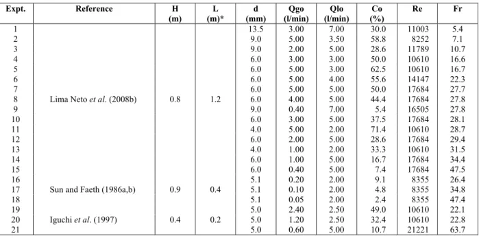
Figure 2: Comparison between model predictions and experimental data of mean liquid velocity given by Lima
Neto et al. (2008b). The numbers (1) to (15) correspond to the experimental conditions shown in Table 1. The normalized radial profiles of u/uo cover a range of z/d from about 30 to 120.
Figure 3: Comparison between model predictions and experimental data of void fraction given by Lima Neto et
482 I. E. Lima Neto
Therefore, the fitted value of γ = 1.0 seems rea-sonable. The simulations were less sensitive to γ than toα. Increasing this parameter to γ = 3.0 (which means more turbulence) resulted in liquid velocities and void fractions of up to about 30% and 10% smaller than those indicated in Figures 2 and 3, re-spectively. It is also interesting to observe that turbu-lence consistently had a higher impact on the liquid velocity than on the void fraction.
The value of λ = 0.6 is smaller than the typical values of 0.7 and 0.8 previously used by Lima Neto (2012b) and Lima Neto (2012a) to predict the liquid volume fluxes induced by bubbly jets and bubble plumes, respectively. The impact of λ on the present model simulations of liquid velocity was very small, yielding variations of less than 3% of the results shown in Figure 2. Nonetheless, λ had a significant impact on void fraction. Increasing this parameter to
λ = 1.0 (which means more spreading of the bubble core) resulted in void fractions of up to about 70% smaller than those shown in Figure 3. On the other hand, decreasing this parameter to λ = 0.4 (which means less spreading of the bubble core) resulted in void fractions of up to about 2 times higher than those shown in Figure 3. Therefore, the spreading ratio variation had a negligible impact on the liquid veloc-ity but a significant impact on the void fraction. This is consistent with the results shown in Table 2 (see
interactions 9 and 10), in which a relatively small drop in λ from 0.7 (used by Lima Neto, 2012b) to 0.6 (used herein) yielded an improvement in the prediction of void fraction from 28 to 19%.
Alternatively, the solution of Eq. (17) using Eq. (13) yielded the following values: α = 0.090, γ = 1.0, and
λ = 0.5, which are close to those obtained by using Eq. (11) instead. Model predictions using these values resulted in standard deviations of 11 and 20% as compared to experimental data of liquid velocity and void fraction, respectively, as well as in coefficients of determination higher than 0.94 for all the cases shown in Figures 2 and 3. This indicates that the use of the drift flux model to predict the two-phase flow structure of vertical bubbly jets provides slightly better results than the use of the average volumetric flux density as an approximation for the initial liquid velocity. On the other hand, the use of the superficial liquid velocity instead of Eq. (11) or Eq. (13) resulted in much larger deviations (> 100%) for some test conditions. Therefore, only the simulations obtained with Eq. (11) will be presented here.
Figure 4 shows a comparison between model pre-dictions and experimental data of bubble velocity of Lima Neto et al. (2008b). The standard deviations were lower than 10% and the coefficient of determi-nation was higher than 0.94 for all the cases (Expt. 1-15 in Table 1).
Figure 4: Comparison between model predictions and experimental data of bubble velocity given by Lima Neto
et al. (2008b). The numbers (1) to (15) correspond to the experimental conditions shown in Table 1. The normal-ized radial profiles of w/uo cover a range of z/d from about 30 to 120. Dashed lines indicate model simulations
Brazilian Journal of Chemical Engineering Vol. 32, No. 02, pp. 475 - 487, April - June, 2015
Note that the normalized radial profiles of w/uo
cover a range of z/d from about 30 to 120. These also give credence to the model and reinforce the idea that bubbly jets behave as self-similar shear flows following Gaussian profiles not only for liquid ve-locity and void fraction (Figures 2 and 3), but also for bubble velocity (Figure 4). It is important to men-tion that model simulamen-tions using Eq. (8) to obtain bubble diameter and then the correlations of Clift et al. (1978) to estimate the terminal velocity for indi-vidual bubbles [instead of Eq. (7)] resulted in higher deviations (up to about 40%) from the experimental results shown in Figure 4, even readjusting the pa-rameters α, γ and λ for a better curve fitting. This sug-gests that bubble swarms rise faster than individual bubbles due to drag reduction, as pointed out by Lima Neto et al. (2008b). Larger terminal velocity than individual particle velocity has also been observed in slurry jets (Zhang et al., 2011).
Figure 5 indicates that model simulations also compared well with the experimental data of liquid velocity given by Sun and Faeth (1986a,b) for dilute bubbly jets. The standard deviations were up to about 20% and the coefficient of determination was higher than 0.98 for all the cases, including tests with den-simetric Froude numbers ranging from 26.4 to 47.4
(see Expt. 16-18 in Table 1). Note that the normalized axial distributions of uc/uo cover a range of z/d from
about 0 to 60.
Model simulations shown in Figure 6 also com-pared well with the experimental data of bubble ve-locity reported by Sun and Faeth (1986a,b) for dilute bubbly jets. The standard deviations of wc/uo were up
to about 15% and the coefficient of determination was higher than 0.99 for all the tests (see Expt. 16-18 in Table 1). Model simulations using Eq. (8) and the correlations of Clift et al. (1978) to estimate the ter-minal bubble velocity [instead of Eq. (7)] resulted in approximately the same deviations (±15%) from the experimental results shown in Figure 6. This indi-cates that Eq. (7) may also be used for modeling the flow structure of dilute bubbly jets.
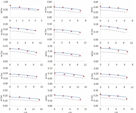
Figure 7 shows another validation of the present model, in which simulated results are compared with experimental data of liquid velocity given by Iguchi et al. (1997) for confined bubbly jets. The standard deviations were lower than 10% and the coefficient of determination was higher than 0.97 for all the cases, which included tests with densimetric Froude numbers ranging from 22.1 to 63.7 (see Expt. 19-21 in Table 1) and normalized axial distributions of uc/uo covering a range of z/d from about 20 to 60.
Figure 5: Comparison between model predictions and experimental data of liquid velocity given by Sun and
Faeth (1986a). The numbers (16) to (18) correspond to the experimental conditions shown in Table 1.
Figure 6: Comparison between model predictions and experimental data of bubble velocity given by Sun and
Faeth (1986a). The numbers (16) to (18) correspond to the experimental conditions shown in Table 1. Dashed lines indicate model simulations using the correlations of Clift et al. (1978) to estimate the terminal velocity for individual bubbles [instead of Eq. (7)].
Figure 7: Comparison between model predictions and experimental data of liquid velocity given by Iguchi et al.
484 I. E. Lima Neto
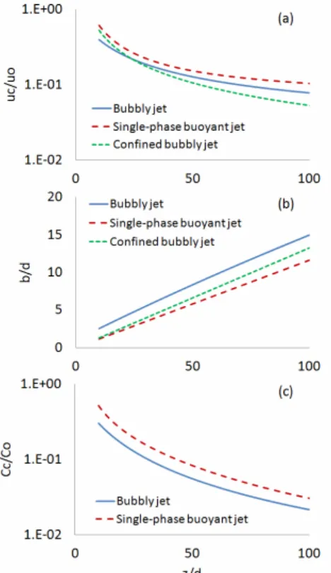
In Figure 8, the present model simulations of cen-terline liquid velocity, jet radius and cencen-terline void fraction are compared to analytical solutions based on Gaussian type self-similarity equations for single-phase buoyant jets reported by Zhang et al. (2011) and empirical correlations for bubbly jets given by Iguchi et al. (1997). The conditions for the bubbly jet simulation using the model proposed herein in-cluded: H = 1.0 m, d = 5 mm, Qgo = Qlo = 3.0 L/min,
Co = 50%, Re = 12732, and Fr = 26.3. The same
value of Fr was used for the single-phase buoyant jet simulations, while the same value of Co was used for
the bubbly jet simulations using the simple correla-tions of Iguchi et al. (1997). Note that Iguchi et al. (1997) only reported correlations for centerline liquid velocity and jet radius.
Figure 8(a) shows the decay of the normalized centerline liquid velocity uc/uo as a function of the
normalized distance from the source z/d. It can be seen that bubbly jets present a decay of uc/uo with z/d
following a slope [uc/uo∼ (z/d)
-3/4
] that is very close to that of single-phase buoyant jets. This is consis-tent with the results presented before, in which the entrainment coefficient of bubbly jets (α = 0.077) is slightly higher than that estimated herein for single-phase buoyant jets (α = 0.075). Thus, bubbly jets and single-phase buoyant jets with the same value of Fr are expected to present approximately the same de-cay of uc/uo with z/d. On the other hand, the
empiri-cal correlation of Iguchi et al. (1997) obtained for confined bubbly jets provided a steeper slope [uc/uo∼
(z/d)-1]. This suggests that the relatively small water levels in the experiments of Iguchi et al. (1997) (see Table 1) caused an earlier decay of the axial liquid velocity, as close to the free surface the jets are ex-pected to bend radially (see Lima Neto et al., 2008a,c). But it is relevant to highlight that, for z/d < 50 [see Figure 8(a)], the simulations using the present model and the empirical correlation of Iguchi et al. (1997) give close results, which is consistent with the results shown in Figure 7. In addition, as a second-order effect, confinement may result in higher turbu-lence levels and, as a consequence, in lower mean liquid velocities along the jet centerline. In fact, the present model simulations for higher momentum amplification factors (γ > 1.0) resulted in steeper slopes than the above-mentioned value (> -3/4). Simi-larly, model simulations for higher entrainment coef-ficients (α > 0.077) also resulted in steeper slopes.
Figure 8(b) shows the increase in the normalized radius b/d as a function of z/d. Observe that for bubbly
jets the radius at the nozzle exit was taken as equal to the nozzle diameter, while no correction for the virtual origin of the flow was considered for the cases of single-phase buoyant jets and confined bub-bly jets. It is seen that unconfined bubbub-bly jets spread approximately linearly with z/d, as do single-phase buoyant jets and confined bubbly jets. However, un-confined bubbly jets spread faster (db/dz ∼ 0.14) than single-phase buoyant jets (db/dz ∼ 0.12) and con-fined bubby jets (db/dz ∼ 0.13). Such results imply that bubble-liquid interactions may play a relevant role in increasing the spreading rate of bubbly jets, as compared to single-phase buoyant jets. On the other hand, the slightly lower spreading rate of confined bubbly jets as compared to unconfined bubbly jets suggests that lateral confinement may restrict the spreading of such flows. Consistently, the above-mentioned spreading rate (db/dz ∼ 0.14) increased by increasing the entrainment coefficient (α > 0.077) and the momentum amplification factor (γ > 1.0).
Figure 8: Simulations using the present model
Brazilian Journal of Chemical Engineering Vol. 32, No. 02, pp. 475 - 487, April - June, 2015
Figure 8(c) shows the decay of the normalized centerline void fraction Cc/Co (or concentration, in
the case of single-phase buoyant jets) as a function of z/d. Again, bubbly jets present a decay of Cc/Co
with z/d following a slope [Cc/Co∼ (z/d)-5/4] which is
very close to that of single-phase buoyant jets. Thus, bubbly jets and single-phase buoyant jets with the same values of Fr are expected to present a similar decay of Cc/Co with z/d. Interestingly, Cc/Co decays
faster than uc/uo [see Figure 8(a)]. Model simulations
for higher entrainment coefficients (α > 0.077) and momentum amplification factors (γ > 1.0) also re-sulted in steeper slopes for the decay of Cc/Co than
the above-mentioned value (> -5/4).
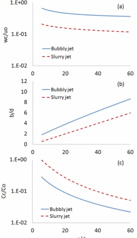
In Figure 9, the present model simulations of cen-terline bubble velocity, jet radius and cencen-terline void fraction are compared to empirical correlations for slurry jets reported by Zhang et al. (2011). The fol-lowing conditions were used for the bubbly jet simulation: H = 1.0 m, d = 9 mm, Qgo = 2.0 l/min,
Qlo = 4.0 l/min, Co = 33.3%, Re = 9431, and Fr = 4.8.
The same value of Fr was used for the slurry jet simulations. Note that here the definition of Fr was modified in order to apply the slurry jet correlations (obtained for 2 < Fr < 6). Hence, for slurry jets, the term
(
ρ ρl− m)
in Eq. (16) was replaced by(
ρ ρs− l)
, in which ρs is the sand density, while for bubbly jets,m
ρ was replaced by ρg.
Figure 9(a) shows the decay of the normalized centerline bubble (or sand) velocity wc/uo as a
function of z/d. Bubbly jets present a decay of wc/uo
with z/d following a slope [uc/uo ∼ (z/d)-1/4] that is
approximately the same of slurry jets. This implies that the buoyancy effects caused by the bubbles and sand particles on the decay of wc/uo are similar. Thus,
bubbly jets and slurry jets with the same Fr are ex-pected to present a similar decay of wc/uo with z/d. It
is also interesting to observe that, as expected, wc/uo
decays much slower than uc/uo [see Figure 8(a)].
Figure 9(b) shows the increase in the normalized radius b/d as a function of z/d. Observe that no cor-rection for the virtual origin of the flow was consid-ered for the slurry jets. It can be seen that bubbly jets spread faster (db/dz ∼ 0.13) than slurry jets (db/dz ∼ 0.10). This probably occurs because bubble-liquid interactions play a more relevant role in increasing the spreading rate than particle-liquid interactions. In fact, bubbles are larger than sand particles and their effect is expected to be stronger. Note that db/dz for the present bubbly jet case is slightly lower than that shown in Figure 8(b).
Figure 9(c) shows the decay of the normalized centerline void fraction Cc/Co (or sand concentration,
in the case of slurry jets) as a function of z/d. Bubbly jets present a decay of Cc/Co with z/d following a
slope [Cc/Co∼ (z/d)-5/4] that is close to that of slurry
jets. Hence, bubbly jets and slurry jets with the same Fr are expected to present a similar decay of Cc/Co
with z/d. The results also confirm that Cc/Co decays
much faster than wc/uo [see Figure 9(a)].
Figure 9: Simulations using the present model
(bub-bly jet) and empirical correlations given by Zhang et al. (2011) (slurry jet): (a) normalized centerline bub-ble (or sand) velocity, (b) normalized radius, and (c) normalized centerline void fraction (or concentra-tion, in the case of the slurry jet).
CONCLUSIONS
opti-486 I. E. Lima Neto
mized values for the entrainment coefficient (α = 0.077), momentum amplification factor (γ = 1.0), and spreading ratio of the bubble core (λ = 0.6) for dif-ferent flow conditions. This resulted in standard de-viations of 10 and 18% between model predictions and experimental data of liquid velocity and void fraction, respectively. The model was also validated with additional data obtained from different experi-mental setups, which yielded deviations between model predictions and experimental data for mean liquid velocity, bubble velocity and void fraction of up to about 20%. This suggests that bubbly jets tend to behave as self-preserving shear flows.
Model predictions of liquid velocity and void fraction were very sensitive to α. On the other hand,
λ significantly affected model predictions of void fraction, while γ presented a small effect on liquid velocity. It was found that bubbly jets induce slightly higher entrainment (α = 0.077) than single-phase buoyant jets (α = 0.075), probably because of the additional entrainment into the wakes of the bubbles. The low value (γ = 1.0) fitted for the momentum amplification factor was consistent with experimen-tal results available in the literature for single-phase jets and confined bubbly jets, which implies that the effect of turbulence on the mean flow structure of bubbly jets is of second order. The fitted value (λ = 0.6) for the spreading ratio of the bubble core was smaller than that obtained in previous bubbly jet studies, but within the ranges reported in the litera-ture for bubble plumes. In fact, a lower value of λ was necessary in the present study in order to fit the radial profiles of void fraction.
The impact of different approaches for evaluation of the liquid velocity at the nozzle exit was also in-vestigated, and the drift flux model provided the best results. Moreover, model comparisons with experi-mental data showed that the use of correlations to describe the increased slip velocity in bubble swarms provided better results than using the classical termi-nal velocity of individual bubbles. This reinforces pre-vious experimental evidence that bubble swarms rise faster than individual bubbles due to drag reduction.
The present model simulations of the axial decay of centerline liquid velocity, bubble velocity, and void fraction (or concentration) indicated a behavior very similar to those of single-phase buoyant jets and slurry jets with the same densimetric Froude numbers. Nonetheless, unconfined bubbly jets presented a slower decay of liquid velocity than confined bubbly jets, probably because of the earlier bend of the liquid flow to the radial direction (close to the free surface) and the higher turbulence levels expected
due to confinement. On the other hand, bubbly jets presented a higher spreading rate than single-phase buoyant jets and slurry jets, which was attributed to bubble-liquid interactions. Lateral confinement also affected the behavior of bubbly jets by lowering their spreading rates, as compared to unconfined bubbly jets. Although some attempts have been made previ-ously by other researchers to model the two-phase flow structure in bubbly jets using computational fluid dynamics (CFD), the agreement between meas-ured and predicted flow characteristics is still quali-tative, especially for higher gas volume fractions. Therefore, the proposed integral model, which is much simpler than CFD models, has the ability to predict the two-phase flow structure in vertical bub-bly jets with gas volume fractions ranging from very low to high. This allows its application in many engi-neering situations involving vertical bubbly jets in reactors, tanks and water bodies. Moreover, this model clearly shows that vertical bubbly jets behave as self-preserving flows, similarly to single-phase jets and plumes.
ACKNOWLEDGMENTS
This work has been financially supported by the National Council for Scientific and Technological Development - CNPq (Project 476430/2011-9).
REFERENCES
Carazzo, G., Kaminski, E. and Tait, S., The route to self-similarity in turbulent jets and plumes. Jour-nal of Fluid Mechanics, 547, 137-148 (2006). Cederwall, K. and Ditmars, J. D., Analysis of
air-bubble plumes. KH-R-24, W. M. Keck Labora-tory of Hydraulics and Water Resources, Division of Engineering and Applied Science, California Institute of Technology, Pasadena, CA (1970). Clift, R., Grace, J. R. and Weber, M. E., Bubbles,
drops and particles. Academic Press, New York (1978).
Iguchi, M., Okita, K., Nakatani, T. and Kasai, N., Structure of turbulent round bubbling jet gener-ated by premixed gas and liquid injection. Int. J. Multiphase Flow, 23(2), 249-262 (1997).
Lima Neto, I. E., Bubble plume modelling with new functional relationships. Journal of Hydraulic Re-search, 50(1), 134-137 (2012a).
Jour-Brazilian Journal of Chemical Engineering Vol. 32, No. 02, pp. 475 - 487, April - June, 2015
nal of Hydraulic Engineering, 138(2), 210-215 (2012b).
Lima Neto, I. E., Zhu, D. Z. and Rajaratnam, N., Air injection in water with different nozzles. Journal of Environmental Engineering, 134(4), 283-294 (2008a).
Lima Neto, I. E., Zhu, D. Z. and Rajaratnam, N., Bubbly jets in stagnant water. Int. J. Multiphase Flow, 34(12), 1130-1141 (2008b).
Lima Neto, I. E., Zhu, D. Z. and Rajaratnam, N., Effect of tank size and geometry on the flow in-duced by circular bubble plumes and water jets. Journal of Hydraulic Engineering, 134(6), 833-842 (2008c).
Lima Neto, I. E., Zhu, D. Z. and Rajaratnam, N., Horizontal injection of gas-liquid mixtures in a water tank. Journal of Hydraulic Engineering, 134(12), 1722-1731 (2008d).
Lima Neto, I. E., Zhu, D. Z., Rajaratnam, N., Yu, T., Spafford, M. and McEachern, P., Dissolved oxy-gen downstream of an effluent outfall in an ice-covered river: Natural and artificial aeration. Jour-nal of Environmental Engineering, 133(11), 1051-1060 (2007).
Milenkovic, R. Z., Sigg, B. and Yadigaroglu, G., Bubble clustering and trapping in large vortices. Part 1: Triggered bubbly jets investigated by phase-averaging. International Journal of Multiphase Flow, 33, 1088-1110 (2007).
Milgram, H. J., Mean flow in round bubble plumes. J. Fluid. Mech., 133, 345-376 (1983).
Morchain, J., Moranges, C. and Fonade, C., CFD modelling of a two-phase jet aerator under influ-ence of a crossflow. Water Res., 34(3), 3460-3472 (2000).
Morton, B. R., Taylor, G. I. and Turner, J. S., Turbu-lent gravitational convection from maintained and instantaneous sources. Proc. R. Soc. London, Ser. A, 234, 1-23 (1956).
Norman, T. L. and Revankar, S. T., Buoyant jet and two-phase jet-plume modeling for application
to large water pools. Nuclear Engineering and Design, 241, 1667-1700 (2011).
Socolofsky, S. A., Bhaumik, T. and Seol, D. G., Dou-ble-plume integral models for near-field mixing in multiphase plumes. J. Hydraul. Eng., 134(6), 772-783 (2008).
Socolofsky, S. A., Crounse, B. C. and Adams, E. E., Multi-phase plumes in uniform, stratified, and flowing environments. Environmental Fluid Me-chanics Theories and Applications, H. Shen, A. Cheng, K.-H. Wang, M. H. Teng, and C. Liu, Eds., ASCE, Reston (2002).
Sun, T. Y. and Faeth, G. M., Structure of turbulent bubbly jets – I. Methods and centerline properties. Int. J. Multiphase Flow, 12(1), 99-114 (1986a). Sun, T. Y. and Faeth, G. M., Structure of turbulent
bubbly jets – II. Phase properties profiles. Int. J. Multiphase Flow, 12(1), 115-126 (1986b).
Suñol, F. and González-Cinca, R., Opposed bubbly jets at different impact angles: Jet structure and bubble properties. Int. J. Multiphase Flow, 36, 682-689 (2010).
Varley, J., Submerged gas-liquid jets: Bubble size prediction. Chem. Eng. Sci., 50(5), 901-905 (1995). Wüest, A., Brooks, N. H. and Imboden, D. M.,
Bub-ble plume modelling for lake restoration. Water Resour. Res., 28(12), 3235-3250 (1992).
Wygnanski, I. and Fiedler, H., Some measurements in the self-preserving jet. J. Fluid. Mech., 38, 577-612 (1969).
Zhang, W. M., Rajaratnam, N. and Zhu, D. Z., Trans-port with Jets and Plumes of Chemicals in the En-vironment. Encyclopedia of Sustainability Sci-ence and Technology, Robert A. Meyers (Ed.), Springer, New York (2011).
Zhang, W. M. and Zhu, D. Z., Bubble characteristics of air–water bubbly jets in crossflow. Int. J. Mul-tiphase Flow, 55(10), 156-171 (2013).