ISSN 0101-8205 www.scielo.br/cam
A smoothing Newton-type method for second-order
cone programming problems based on a new
smoothing Fischer-Burmeister function
LIANG FANG1∗ and ZENGZHE FENG2 1College of Mathematics and System Science, Taishan University,
271021, Tai’an, P.R. China
2College of Information Engineering, Taishan Medical University,
271016, Tai’an, P.R. China
E-mails: [email protected] / [email protected]
Abstract. A new smoothing function of the well known Fischer-Burmeister function is given. Based on this new function, a smoothing Newton-type method is proposed for solving second-order cone programming. At each iteration, the proposed algorithm solves only one system of linear equations and performs only one line search. This algorithm can start from an arbitrary point and it is Q-quadratically convergent under a mild assumption. Numerical results demonstrate the effectiveness of the algorithm.
Mathematical subject classification: 90C25, 90C30, 90C51, 65K05, 65Y20.
Key words: second-order cone programming, smoothing method, interior-point method, Q-quadratic convergence, central path, strong semismoothness.
1 Introduction
The second order cone (SOC) inRn(n ≥ 2), also called the Lorentz cone or the ice-cream cone, is defined as
Qn =(x1;x2)|x1∈R,x2∈Rn−1 and x1≥ kx2k) ,
here and below,k ∙ krefers to the standard Euclidean norm,nis the dimension ofQn, and for convenience, we write x = (x1;x2) instead of(x1,x2T)T. It is
easy to verify that the SOCQnis self-dual, that is
Qn=Q∗n =
s ∈Rn:sTx ≥0, for allx ∈Qn .
We may often drop the subscripts if the dimension is evident from the context. For any x = (x1;x2),y = (y1;y2) ∈ R×Rn−1, their Jordan product is
defined as [5]
x◦y= xTy;x1y2+y1x2
.
Second-order cone programming (SOCP) problems are to minimize a linear function over the intersection of an affine space with the Cartesian product of a finite number of SOCs. The study of SOCP is vast important as it covers linear programming, convex quadratic programming, quadratically constraint convex quadratic optimization as well as other problems from a wide range of applications in many fields, such as engineering, control, optimal control and design, machine learning, robust optimization and combinatorial optimization and so on [13, 24, 4, 23, 29, 22, 18, 10, 11].
Without loss of generality, we consider the SOCP problem with a single SOC
(PSOCP) min
hc,xi : Ax =b,x ∈Q (1)
and its dual problem
(DSOCP) maxhb,yi : ATy+s =c,s ∈Q,y∈Rm , (2)
wherec ∈ Rn,A ∈ Rm×n andb ∈ Rm, with an inner product h∙,∙i, are given data. x ∈ Qis variable and the setQis an SOC of dimensionn. Note that our analysis can be easily extended to the general case with Cartesian product of SOCs.
We call x ∈ Q primal feasible if Ax = b. Similarly(y,s) ∈ Rm ×Q is called dual feasible if ATy
+s = c. For a given primal-dual feasible point (x,y,s)∈Q×Rm
×Q,hx,siis called the duality gap due to the well known weak dual theorem, i.e.,hx,si ≥0, which follows that
Let us note thathx,si =0 is sufficient for optimality of primal and dual feasible (x,y,s)∈Q×Rm×Q.
Throughout the paper, we make the following Assumption:
Assumption 2.1. Both (PSOCP) and its dual (DSOCP) are strictly feasible. It is well known that under the Assumption 2.1, the SOCP is equivalent to its optimality conditions:
Ax =b,
ATy+s =c,
x◦s =0, x,s ∈Q, y ∈Rm,
(3)
wherehx,si =0 is usually referred to as the complementary condition.
There are an extensive literature focusing on interior-point methods (IPMs) for (PSOCP) and (DSOCP) (see, e.g., [1, 17, 6, 23, 16, 11] and references therein). IPMs typically deal with the following perturbation of the optimality conditions:
Ax =b,
ATy+s =c,
x◦s =μe, x,s ∈Q, y ∈Rm,
(4)
whereμ >0 ande=(1;0)∈R×Rn−1is identity element. This set of
condi-tions are called thecentral path conditionsas they define a trajectory approach-ing the solution set asμ↓ 0. Conventional IPMs usually apply a Newton-type method to the equations in (4) with a suitable line search dealing with constraints x ∈Qands ∈Qexplicitly.
locally superlinearly/quadratically convergent without strict complementarity. Moreover, the smoothing methods available are mostly for solving the comple-mentarity problems [2, 3, 19, 20, 7, 8], but there is little work on smoothing methods for the SOCP.
Under certain assumptions, IPMs and smoothing methods are globally conver-gent in the sense that every limit point of the generated sequence is a solution of optimality conditions (3). However, with the exception of the infeasible IPMs [2, 21, 20], they need a feasible starting point.
Fukushima, Luo and Tseng studied Lipschitzian and differential properties of several typical smoothing functions for second-order cone complementar-ity problems. They derived computable formulas for their Jacobians, which provide a theoretical foundation for constructing corresponding non-interior point methods. The purpose of this paper is just to present such a non-interior point method for problem (PSOCP), which employs a new smoothing func-tion to characterize the central path condifunc-tions. We stress on the demonstrafunc-tion of the global convergence and locally quadratic convergence of the proposed algorithm.
The new smoothing algorithm to be discussed here is based on perturbed opti-mality conditions (4) and the main difference from IPMs is that we reformulate (4) as a smoothing linear system of equations. It is shown that our algorithm has the following good properties:
(i) The algorithm can start from an arbitrary initial point;
(ii) The algorithm needs to solve only one linear system of equations and perform only one line search at each iteration;
(iii) The algorithm is globally and locally Q-quadratically convergent under mild assumption, without strict complementarity. The result is stronger than the corresponding results for IPMs.
x −y ∈ Qory−x ∈ Q(respectively,x −y ∈ intQory−x ∈intQ, where intQdenotes the interior ofQ). R+(R++)denotes the set of nonnegative (pos-itive) reals. Forx ∈ Rn with eigenvaluesλ1andλ2, we can define the
Frobe-nius norm
kxkF :=
q
λ21+λ22=ptr(x2).
Since both eigenvalues ofeare equal to one,kekF =
√
2. For anyx,y ∈ Rn, the Euclidean inner product and norm are denoted byhx,yi =xTyandkxk =
√
xTx respectively.
The paper is organized as follows. In Section 2, we give the equivalent for-mulation of the perturbed optimality conditions and some preliminaries. A smoothing function associated with the SOCQand its properties are given in Section 3. In Section 4, we describe our algorithm. The convergence of the new algorithm is analyzed in Section 5. Numerical results are shown in Section 6.
2 Preliminaries
For any vectorx =(x1;x2)∈R×Rn−1, we define its spectral decomposition
associated with SOCQas
x =λ1u1+λ2u2, (5)
where the spectral values λi and the associated spectral vectors ui of x are
given by
λi =x1+(−1)i+1kx2k, (6)
ui =
1 2
1;(−1)i+1 x2 kx2k
, x26=0;
1
2(1;(−1)
i+1ω), x 2=0,
(7)
for i = 1,2, with any ω ∈ Rn−1 such that kωk = 1. If x2 6= 0, then the
decomposition (5) is unique. Some interesting properties ofλ1, λ2andu1,u2
Property 2.1. For any x = (x1;x2) ∈ R×Rn−1, the spectral values λ1,
λ2and spectral vectorsu1,u2as given by (6) and (7), have the following
prop-erties:
(i) u1+u2=e.
(ii) u1andu2are idempotent under the Jordan product, i.e.,ui2=ui,i=1,2.
(iii) u1andu2are orthogonal under the Jordan product, i.e.,u1◦u2=0, and
have length√2/2.
(iv) λ1, λ2 are nonnegative (respectively, positive) if and only if x ∈ Q
(re-spectively,x ∈intQ).
Given an elementx =(x1;x2)∈Rn, we define the arrow-shaped matrix
Lx =
x1 x2T x2 x1I
!
,
whereI represents the(n−1)×(n−1)identity matrix. It is easy to verify that x ◦s =Lx◦s = Ls ◦x =LxLsefor anys ∈Rn. Moreover,Lx is symmetric
positive definite if and only ifx ∈intQ, i.e.,x ≻Q 0.
3 A smoothing function associated with the SOCQand its properties
First, let us introduce a smoothing function. In [7], it has been shown that the vector valued Fischer-Burmeister functionφF B(x,s):Rn×Rn →Rndefined
by
φF B(x,s)=x+s−
p
x2+s2 (8)
satisfies the following important property
φF B(x,s)=0⇐⇒ x ∈Q,s ∈Q,x ◦s =0. (9)
We now smoothing the function φF B, so that we get a characterization of
the central path conditions (4). By smoothing the symmetrically perturbed φF B, we obtain the new vector-valued function8:D→Rn, defined by
8(μ,x,s)= 1 2μ
μ2e−(x−μe)2−(s−μe)2, (10) whereD= {(μ,x,s)∈R++×Rn×Rn :μ >k√x2+s2k
F}.
Proposition 3.1. For any(μ1,x,s), (μ2,x,s)∈D,
k8(μ1,x,s)−8(μ2,x,s)kF <|μ1−μ2|.
Proof. For any (μ1,x,s), (μ2,x,s) ∈ D, without loss of generality, we
assumeμ1≥μ2>
√
x2+s2. Thus, we have
k8(μ1,x,s)−8(μ2,x,s)kF
= k −x
2
+s2 2μ1 −
μ1
2 e+
x2+s2 2μ2 +
μ2
2 ekF
= k(μ1−μ2)(x
2
+s2)
2μ1μ2 −
μ1−μ2
2 ekF
≤ k(μ1−μ2)(x
2
+s2)
2μ1μ2 k F + |
μ1−μ2
2 |
= |μ21−μ2| μ1μ2 k
x2+s2kF+|
μ1−μ2|
2
≤ |μ21−μ2| μ1μ2 k
p
x2
+s2
kFk
p
x2
+s2
kF+|
μ1−μ2|
2
< |μ1−μ2| 2μ1μ2
μ1μ2+|
μ1−μ2|
2
= |μ1−μ2|,
which completes the proof.
for any(μ,x,s) ∈ D. This property plays an important role in the analysis of the quadratic convergence of our smoothing Newton method. Semismooth-ness is a generalization concept of smoothSemismooth-ness, which was originally introduced in [15] and then extended by L. Qi in 1993. Semismooth functions include smooth functions, piecewise smooth functions, convex and concave functions, etc. The composition of (strongly) semismooth functions is still a (strongly) semismooth function.
Definition 3.1. Suppose that H : Rn → Rm is a locally Lipschitz contin-uous function. H is said to be semismooth at x ∈ Rn if H is directionally differentiable at x and for any V ∈∂H(x + △x)
H(x+ △x)−H(x)−V(△x)=o(k△xk).
H is said to be p-order(0 < p < ∞) semismooth at x if H is semismooth at x and
H(x+ △x)−H(x)−V(△x)=O(k△xk1+p).
In particular, H is called strongly semismooth at x if H is 1-order semismooth at x.
The following concept of a smoothing function of a nondifferentiable func-tion was introduced by Hayashi, Yamashita and Fukushima [8].
Definition 3.2. A function H :Rn→Rmis said to be a semismooth (respect-ively, p-order semismooth) function if it is semismooth (respect(respect-ively, p-order semismooth) everywhere inRn.
In fact, the function 8(μ,x,s) given by (10) is a smoothing function of φF B(x,s). Thus, we can solve a family of smoothing subproblems8(μ,x,s)=
0 forμ >0 and obtain a solution of8F B(x,s)=0 by lettingμ↓0.
Definition 3.3 [8]. For a nondifferentiable function g :Rn → Rm, we con-sider a function gμ:Rn→Rm with a parameterμ >0that has the following properties:
(ii) lim
μ↓0gμ(x)=g(x)for any x ∈R n.
Such a functiongμis called a smoothing function ofg.
Theorem 3.1. For any x,s ∈Rn, letw :=√x2
+s2whose spectral decom-position associated with SOCQisw = λ1u1+λ2u2. Ifμ > k
√
x2+s2k F, then the following results hold:
(i) w<0; (ii) μe≻w; (iii) μ2e≻w2.
Proof. Assume the spectral decomposition of w associated with SOC Q is w=λ1u1+λ2u2. Fromμ >k
√
x2+s2k
F we have
μ >kpx2+s2k
F = kλ1u1+λ2u2kF =
q
λ21+λ22≥max{λ1, λ2}. (11)
Thus, we have 0≤λi < μ,i =1,2, which means that (i) holds. By
0≤λi < μ,i =1,2, μe−w=(μ−λ1)u1+(μ−λ2)u2≻0,
which yields (ii), and μ2e−w2 = (μ2 −λ21)u1+(μ2−λ22)u2 ≻ 0, which
gives (iii).
Now, we give the main properties of8(μ,x,s):
Theorem 3.2. (i) 8(μ,x,s) is globally Lipschitz continuous for any (μ,
x,s) ∈ D. Moreover, 8(μ,x,s) is continuously differentiable at any (μ,
x,s)∈Dwith its Jacobian
8′(μ,x,s)=
1 2μ2 x
2
+s2
−μ2e
I − 1
μLx
I − 1
μLs
. (12) (ii) lim
μ↓08(μ,x,s)=φF B(x,s)for any(x,s)∈R n
Proof. (i) It is not difficult to show that8(μ,x,s)is globally Lipschitz con-tinuous, and continuously differentiable at any(μ,x,s) ∈ D. Now we prove (12). For any(μ,x,s)∈D, from (10) and by simply calculation, we have
8′μ(μ,x,s) = 1 2μ2(x
2
+s2−μ2e), 8′x(μ,x,s) = I − 1
μLx,
8′s(μ,x,s) = I − 1
μLs,
which yield (12).
Next, we prove (ii). For any x = (x1;x2) ∈ R×Rn−1 ands = (s1;s2) ∈ R×Rn−1, denote w
= √x2+s2 whose spectral decomposition associated
with SOCQ isw = λ1u1+λ2u2. From Theorem 3.1, we have w < 0, and
0≤λi ≤μ,i =1,2.Therefore, we have
k8(μ,x,s)−φF B(x,s)kF
= 1 2μ
μ2e−(x−μe)2−(s−μe)2−x−s+px2+s2
F = 1 2μ(x
2
+s2+μ2e)−px2
+s2
F = 1 2μ(
p
x2+s2−μe)2
F = 1 2μ
[(λ1−μ)u1+(λ2−μ)u2]2
F = 1 4μ
(λ1−μ)2+(λ2−μ)2
≤ 41
μ μ
2
+μ2
= 1
2μ→0, whenμ↓0. Thus, we have lim
μ↓08(μ,x,s) =φF B(x,s). Therefore, it follows from (i) and
4 Description of the algorithm
Based on the smoothing function (10) introduced in the previous section, the aim of this section is to propose the smoothing Newton-type algorithm for the SOCP and show the well-definedness of it under suitable assumptions.
Letz := (μ,x,c− ATy)
∈ D. By using the smoothing function (10), we define the functionG(μ,x,y):R×Rn×Rm →R×Rm×Rnby
G(z):=
μ
Ax−b
8(μ,x,c−ATy)
. (13)
In view of (9) and (13),z∗:=(μ∗,x∗,y∗)is a solution of the systemG(z)=0 if and only if(x∗,y∗,c−ATy∗)solves the optimality conditions (3).
It is well-known that problems (PSOCP) and (DSOCP) are equivalent to (13) [1, 20]. Therefore,z∗is a solution ofG(z)=0 if and only if(x∗,y∗,c−ATy∗) is the optimal solution of (PSOCP) and (DSOCP). Then we can apply Newton’s method to the nonlinear system of equationsG(z)=0.
Letγ ∈(0,1)and define the functionβ :Rn+m+1→R+by β(z):=γmin
1, kG(z)k2 . (14)
Now we are in the position to give a formal description of our algorithm.
Algorithm 4.1. (A smoothing Newton-type method forSOCP).
Step 0. Choose constants δ ∈ (0,1), σ ∈ (0,1), and μ0 ∈ R++, and let
ˉ
z := (μ0,0,0) ∈ D. Let (x0,y0) ∈ Rn ×Rm be arbitrary initial point and z0:=(μ0,x0,y0). Chooseγ ∈(0,1)such thatγ μ0<1/2. Setk :=0. Step 1. IfG(zk)=0, then stop. Else, letβk :=β(zk).
Step 2. Compute1zk :=(1μk, 1xk, 1yk)by solving the following system of
linear equations
G(zk)+G′(zk)1zk =βkzˉ. (15)
Step 3. Letνk be the smallest nonnegative integerνsuch that
kG(zk+δν1zk)k2≤
1−σ (1−2γ μ0)δν
Letλk :=δνk.
Step 4. Setzk+1:=zk+λk1zk andk :=k+1. Go to step 1.
In order to analyze our algorithm, we study the Lipschitzian, smoothness and differential properties of the function G(z) given by (13). Moreover, we de-rive the computable formula for the Jacobian of the functionG(z)and give the condition for the Jacobian to be nonsingular.
Throughout the rest of this paper, we make the following assumption:
Assumption 4.1. The matrixAhas full row rank, i.e., all the row vectors ofA are linearly independent.
Lemma 4.1 [7]. For any x,s ∈Rnand anyω≻Q 0, we have
ω2≻Q x2+s2 ⇒Lω−Lx ≻0, Lω−Ls ≻0, (Lω−Lx)(Lω−Ls)≻0. (17) Moreover,(17)remains true when “≻” is replaced by “<” everywhere.
Theorem 4.1. Let z := (μ,x,y) ∈ D and G : D → Dbe defined by(13). Then the following results hold.
(i) G is globally Lipschitz continuous, and continuously differentiable at any z:=(μ,x,y)∈Dwith its Jacobian
G′(z)=
1 0 0
0 A 0
I− 1 2μ2
h
x2+ c−ATy2 −μ2e
i
I− 1 μLx −
I− 1
μLc−ATy
AT
. (18)
(ii) Under Assumption4.1, G′(z)is nonsingular for anyμ >0.
Proof. By Theorem 3.1, we can easily show that (i) holds. Now we prove (ii). For any fixedμ >0, let
1z:=(1μ, 1x, 1y)∈R×Rn×Rm.
It is sufficient to prove that the linear system of equations
has only zero solution, i.e.,1μ =0,1x = 0 and1y = 0. By (18) and (19), we have
1μ=0, (20)
A1x =0, (21)
I − 1
μLx
1x−
I − 1
μL(c−ATy)
AT1y =0. (22)
Since
e2≻
x μ 2 +
c−ATy
μ
2
,
It follows from Lemma 4.1 that
I − 1
μLx ≻0, I − 1
μL(c−ATy)≻0,
I − 1
μLx I − 1
μL(c−ATy)
≻0. (23)
Premultiplying (23) by1xT I
−μ1L(c−ATy)
−1
and taking into accountA1x = 0, we have
1xT
I − 1
μL(c−ATy)
−1
I − 1
μLx
1x =0. (24)
Denote
1x˜ =
I − 1
μL(c−ATy)
−1
1x. (25)
From (24), we obtain
1x˜T
I − 1
μLx I −
1
μL(c−ATy)
1x˜ =0. (26)
By (23), I −μ1Lx
I −μ1L(c−ATy)
is positive definite. Therefore, (26) yields 1x˜ =0, and it follows from (25) that1x =0. Since Ahas full row rank, (21) implies1y =0. Thus the linear system of equations (19) has only zero solution, and henceG′(z)is nonsingular. Thus, the proof is completed.
By Theorem 4.1, we can show that Algorithm 4.1 is well-defined.
Proof. Since A has full row rank, it follows from Theorem 4.1 that G′(zk)
is nonsingular for anyμk > 0. Therefore, Step 2 is well-defined at thekth
iteration. Then by following the proof of Lemma 5 in [20], we can show the
well-definedness of Step 3. The proof is completed.
5 Convergence analysis
In this section, we analyze the global and local convergence properties of Al-gorithm 4.1. It is shown that any accumulation point of the iteration sequence is a solution of the systemG(z) = 0. If the accumulation pointz∗ satisfies a nonsingularity assumption, then the iteration sequence converges to z∗ locally Q-quadratically without any strict complementarity assumption. To show the global convergence of Algorithm 4.1, we need the following Lemma (see [20], Proposition 6).
Lemma 5.1. Suppose that Assumption 4.1 holds. For any z˜ := (u˜,x˜,y˜) ∈
R++×Rn×Rm, and G′(z˜)is nonsingular, then there exists a closed neigh-borhood N(z˜) of z and a positive number˜ αˉ ∈ (0,1] such that for any z =
(u,x,y)∈N(z˜)and allα∈ [0,αˉ], we have u∈R++, G′(z)is invertible and
kG(z+α1z)k2≤1−σ (1−2γ μ0)α
kG(z)k2. (27)
Theorem 5.1. Suppose that Assumption4.1holds and that{zk}is the iteration sequence generated by Algorithm4.1. Then the following results hold.
(i) μk ∈R++and zk ∈2for any k≥0, where
2= {z =(μ,x,y)∈D:μ≥β(z)μ0}. (28)
(ii) Any accumulation point z∗ := (μ∗,x∗,y∗) of {zk} is a solution of G(z)=0.
Proof. Suppose thatμk >0. It follows from (15) and Step 4 that
1μk = −μk+βkμ0, (29)
Substituting (29) into (30), we have
μk+1=μk−λkμk+λkβkμ0=(1−λk)μk+λkβkμ0>0, (31)
which, together withμ0 >0 andλk =δνk ∈ (0,1)implies thatμk ∈R++for anyk ≥0.
Now we provezk ∈2for anyk≥0 by induction. Since
β0=β(z0)=γmin
1, kG(z0)k2 ≤γ ∈(0,1),
it is easy to see thatz0∈2. Suppose thatzk ∈2, then
μk ≥βkμ0. (32)
We consider the following two cases:
Case (I): IfkG(zk)k>1, then
βk =γ . (33)
Since βk+1 = γ min{1,kG(zk+1)k2} ≤ γ, it follows from (16), (31), (32)
and (33) that
μk+1−βk+1μ0≥(1−λk)βkμ0+λkβkμ0−γ μ0=βkμ0−γ μ0=0. (34) Case (II): IfkG(zk)k ≤1, then
βk =γkG(zk)k2. (35)
By (16), we havekG(zk+1)k ≤ kG(zk)k ≤1. From (31), (35), and taking into
accountβk+1=γkG(zk+1)k2, we have
μk+1−βk+1μ0 = (1−λk)μk+λkβkμ0−γ μ0kG(zk+1)k2
≥ (1−λk)βkμ0+λkβkμ0−γ μ0kG(zk)k2
= βkμ0−γ μ0kG(zk)k2
= 0. (36)
Now, we prove (ii). Without loss of generality, we assume that{zk}converges
toz∗ ask → +∞. Since{kG(z
k)k}is monotonically decreasing and bounded
from below, it follows from the continuity ofG(∙)that{kG(zk)k}converges to a
nonnegative numberG(z∗). Then by the definition ofβ(∙), we obtain that{βk}
converges to
β∗=γmin1, kG(z∗)k2 . It follows from (15) and Theorem 5.1 (i) that
0< μk+1=(1−λk)μk+λkβkμ0≤μk,
which implies that{μk}converges toμ∗. IfkG(z∗)k = 0, then we obtain the
desired result. In the following, we supposekG(z∗)k > 0. By Lemma 4.1, 0 < β∗μ0 ≤ μ∗. It follows from Theorem 4.1 that G′(z∗) exists and it is
invertible. Hence, by Lemma 5.1, there exists a closed neighborhoodN(z˜)of ˜
zand a positive numberαˉ ∈(0,1]such that for anyz =(μ,x,y)∈N(z˜)and allα ∈ [0,αˉ], we haveμ∈R++,G′(z)is invertible and
kG(z+α1z)k2≤1−σ (1−2γ μ0)α
kG(z)k2. (37) Therefore, for a nonnegative integerνˉ such thatδνˉ ∈ (0,αˉ], for all sufficiently largek, we have
kG(zk+δνˉ1zk)k2≤
1−σ (1−2γ μ0)δνˉ
kG(zk)k2.
For all sufficiently largek, sinceλk =δνk ≥δνˉ, it follows from (16) that
kG(zk+δνˉ1zk)k2 ≤
1−σ (1−2γ μ0)λk
kG(zk)k2
≤ 1−σ (1−2γ μ0)δνˉ
kG(zk)k2.
This contradicts the fact that the sequence{kG(zk)k}converges tokG(z∗)k>0.
This completes the proof.
To establish the locally Q-quadratic convergence of our smoothing Newton method, we need the following assumption:
Assumption 5.1. Assume that z∗ satisfies the nonsingularity condition, i.e., allV ∈∂G(z∗)are nonsingular.
Theorem 5.2. Suppose that Assumption4.1holds and that z∗ is an accumu-lation point of the iteration sequence {zk} generated by Algorithm 4.1. If Assumption5.1holds, then:
(i) λk ≡1for all zk sufficiently close to z∗;
(ii) {zk}converges to z∗Q-quadratically, i.e.,kzk+1−z∗k = O(kzk−z∗k2); moreover,μk+1=O(μ2k).
Proof. By using Lemma 3.1 and Theorem 4.1, we can prove the theorem similarly as in Theorem 8 of [20]. For brevity, we omit the details here.
6 Numerical results
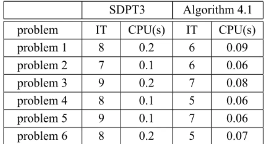
In this section, we conducted some numerical experiments to evaluate the ef-ficiency of Algorithm 4.1. All these experiments were performed on an IBM notebook computer R40e with Intel(R) Pentium(R) 4 CPU 2.00 GHz and 512 MB memory. The operating system was Windows XP SP2 and the implemen-tations were done in MATLAB 7.0.1. For comparison purpose, we also use SDPT3 solver [12] which is an IPM for the SOCP.
For simplicity, we randomly generate six test problems with sizem=50 and n=100. To be specific, we generate a random matrix A∈Rm×nwith full row rank and random vectors
x ∈intQ, s ∈intQ, y∈Rm, and then let b:= Ax and c:= ATy+s.
Thus the generated problems (PSOCP) and (DSOCP) have optimal solutions and their optimal values coincide, because the set of strictly feasible solutions of (PSOCP) and (DSOCP) are nonempty. Letx0= e∈ Rn andy0 =0 ∈Rm
be initial points. The parameters used in Algorithm 4.1 were as follows:
μ0=0.01, σ =0.35, δ=0.65 andγ =0.90.
We usedkH(z)k ≤10−5as the stopping criterion.
SDPT3 Algorithm 4.1 problem IT CPU(s) IT CPU(s)
problem 1 8 0.2 6 0.09
problem 2 7 0.1 6 0.06
problem 3 9 0.2 7 0.08
problem 4 8 0.1 5 0.06
problem 5 9 0.1 7 0.06
problem 6 8 0.2 5 0.07
Table 1 – Comparison of Algorithm 4.1 and SDPT3 on SOCPs.
Acknowledgments. The work is supported by National Natural Science Foundation of China (10571109, 10971122), Natural Science Foundation of Shandong (Y2008A01), Scientific and Technological Project of Shandong Province (2009GG10001012), the Excellent Young Scientist Foundation of Shandong Province (BS2011SF024), and Project of Shandong Province Higher Educational Science and Technology Program (J10LA51). The authors would like to thank the anonymous referees for their valuable comments and sugges-tions on the paper, which have considerably improved the paper.
REFERENCES
[1] F. Alizadeh and D. Goldfarb, Second-order cone programming. Mathematical Programming,95(2003), 3–51.
[2] B. Chen and N. Xiu,A global linear and local quadratic non-interior continuation method for nonlinear complementarity problems based on Chen-Mangasarian
smoothing functions. SIAM Journal on Optimization,9(1999), 605–623.
[3] J. Chen,Two classes of merit functions for the second-order cone complementarity
problem. Math. Meth. Oper. Res.,64(2006), 495–519.
[4] R. Debnath, M. Muramatsu and H. Takahashi, An Efficient Support Vector Ma-chine Learning Method with Second-Order Cone Programming for Large-Scale
Problems. Applied Intelligence,23(2005), 219–239.
[5] J. Faraut and A. Koranyi,Analysis on symmetric cones. Oxford University Press, London and New York, 1994, ISBN: 0-198-53477-9.
[7] M. Fukushima, Z. Luo and P. Tseng,Smoothing functions for second-order-cone
complimentarity problems. SIAM J. Optim.,12(2) (2002), 436–460.
[8] S. Hayashi, N. Yamashita and M. Fukushima,A combined smoothing and
regular-ized method for monotone second-order cone complementarity problems. SIAM
Journal on Optimization,15(2005), 593–615.
[9] K. Hotta and A. Yoshise, Global convergence of a class of non-interior-point algorithms using Chen-Harker-Kanzow functions for nonlinear complementarity
problems. Discussion Paper Series No. 708, Institute of Policy and Planning
Sci-ences, University of Tsukuba, Tsukuba, Ibaraki 305, Japan, December 1996. CMP 98:13.
[10] Y. Kanno and M. Ohsaki,Contact Analysis of Cable Networks by Using
Second-Order Cone Programming. SIAM J. Sci. Comput.,27(6) (2006), 2032–2052.
[11] Y.J. Kuo and H.D. Mittelmann,Interior point methods for second-order cone
pro-gramming and OR applications. Computational Optimization and Applications,
28(2004), 255–285.
[12] Y. Liu, L. Zhang and Y. Wang,Analysis of a Smoothing Method for Symmetric
Cone Linear Programming. J. Appl. Math. and Computing,22(1-2) (2006), 133–
148.
[13] M.S. Lobo, L. Vandenberghe, S. Boyd and H. Lebret,Applications of second-order
cone programming. Linear Algebra and its Applications,284(1998), 193–228.
[14] C. Ma and X. Chen,The convergence of a one-step smoothing Newton method
for P0-NCP based on a new smoothing NCP-function. Journal of Computational
and Applied Mathematics,216(2008), 1–13.
[15] R. Miffin, Semismooth and semiconvex functions in constrained optimization. SIAM Journal on Control and Optimization,15(1977), 957–972.
[16] Y.E. Nesterov and M.J. Todd,Primal-dual Interior-point Methods for Self-scaled
Cones. SIAM J. Optim.,8(2) (1998), 324–364.
[17] J. Peng, C. Roos and T. Terlaky,Primal-dual Interior-point Methods for
Second-order Conic Optimization Based on Self-Regular Proximities. SIAM J. Optim.,
13(1) (2002), 179–203.
[18] X. Peng and I. King,Robust BMPM training based on second-order cone
pro-gramming and its application in medical diagnosis. Neural Networks,21(2008),
[19] L. Qi and D. Sun,Improving the convergence of non-interior point algorithm for
nonlinear complementarity problems. Mathematics of Computation, 69(2000),
283–304.
[20] L. Qi, D. Sun and G. Zhou,A new look at smoothing Newton methods for
non-linear complementarity problems and box constrained variational inequalities.
Mathematical Programming,87(2000), 1–35.
[21] B.K. Rangarajan,Polynomial Convergence of Infeasible-Interior-Point Methods
over Symmetric Cones. SIAM J. Optim.,16(4) (2006), 1211–1229.
[22] T. Sasakawa and T. Tsuchiya,Optimal Magnetic Shield Design with Second-order
Cone Programming. SIAM J. Sci. Comput.,24(6) (2003), 1930–1950.
[23] S.H. Schmieta and F. Alizadeh,Extension of primal-dual interior point algorithms
to symmetric cones, Mathematical Programming, Series A96(2003), 409–438.
[24] P.K. Shivaswamy, C. Bhattacharyya and A.J. Smola,Second Order Cone
Program-ming Approaches for Handling Missing and Uncertain Data. Journal of Machine
Learning Research,7(2006), 1283–1314.
[25] D. Sun and J. Sun,Strong Semismoothness of the Fischer-Burmeister SDC and
SOC Complementarity Functions. Math. Program., Ser. A103(2005), 575–581.
[26] K.C. Toh, R.H. Tütüncü and M.J. Todd,SDPT3 Version 3.02-A MATLAB software
for semidefinite-quadratic-linear programming,
http://www.math.nus.edu.sg/∼mattohkc/sdpt3.html, 2002.
[27] P. Tseng,Error bounds and superlinear convergence analysis of some
Newton-type methods in optimization, in: G. Di Pillo, F. Giannessi (Eds.), Nonlinear
Optimization and Related Topics, Kluwer Academic Publishers, Boston, (2000), pp. 445–462.
[28] S. Xu, The global linear convergence and complexity of a non-interior path-following algorithm for monotone LCP based on Chen-Harker-Kanzow-Smale
smooth functions. Preprint, Department of Mathematics, University of
Washing-ton, Seattle, WA 98195, February (1997).
[29] S. Yan and Y. Ma,Robust supergain beamforming for circular array via