SEA SURFACE TEMPERATURE DISTRIBUTION IN THE AZORES REGION.
PART I: AVHRR IMAGERY AND IN SITU DATA PROCESSING
VIRGINIE LAFON, ANA MARTINS, MIGUEL FIGUEIREDO, MARGARIDA A. MELO
RODRIGUES, IGOR BASHMACHNIKOV, ANA MENDONÇA, LUIS MACEDO & NERI
GOULART
LAFON V., A. MARTINS, M. FIGUEIREDO, M.A. MELO RODRIGUES, I. BASHMACHNIKOV,A.MENDONÇA,L.MACEDO &N.GOULART. 2004. Sea surface temperature distribution in the Azores region. Part I: AVHRR imagery and in situ data processing. Arquipélago. Life and Marine Sciences 21A: 1-18.
Sixteen months of 1.1 km resolution NOAA-12, -14, and -16 data for the Azores region are investigated. Advanced Very High Resolution Radiometer (AVHRR) derived sea surface temperature (SST) is compared to an extensive in situ temperature measurement database, mainly constituted during fisheries campaigns. This comparison shows that SST maps include numerous pixels with temperature values below the range observed for the Azores. Low temperatures are attributed in literature to pixel contamination by cloud neighbouring and these are usually removed by eroding pixels around clouds. Results of this study show that running an erosion filter removes only two thirds of the contaminated pixels. Remnant clouds are filtered inputting threshold values to SST 8-day temperature histograms. Based on a comparison of the SST values derived on an image-by-image basis, it is also demonstrated that differences among the sensors are lower than the measurement accuracy, whilst, on the contrary, nighttime and daytime SST distributions are statistically different. Based on monthly and 15-day average computations at nighttime, AVHRR-derived SST distribution in the Azores and associated dominant space and time scales are proposed in the second part of this paper (SST distribution in the Azores region. Part II: Space and time variability and its relation to North Atlantic Oscillation).
Virginie Lafon (e-mail: [email protected]), Ana Martins, Miguel Figueiredo, Margarida Melo Rodrigues, Igor Bashmachnikov, Ana Mendonça, Luis Macedo & Neri Goulart, Centro do IMAR (Instituto do Mar) da Universidade dos Açores, Departamento de Oceanografia e Pescas, Cais de Santa Cruz, PT - 9901-862 Horta, Açores, Portugal. INTRODUCTION
Simple characteristics of the Azores waters, such as water temperature seasonal variability and mean anomaly fields, need to be precisely measured to better understand the climate in the North Atlantic. The Azores archipelago (Fig. 1) is situated in the inter-gyre region of the eastern North Atlantic, with the southern edge of the subpolar gyre located at about 50º N, and the northern edge of the subtropical gyre located at about 34º N (MAILLARD 1986). The Gulf Stream current feeds the Azores area. Its southeastern branch crosses the Atlantic ridge at about 45º W and between 32º and 35º N generating the
eastward-flowing Azores current (AzC) (KLEIN & SIEDLER 1989). Westward surface counterflows have been also reported to the northern (CROMWELL et al. 1996) and to the southern (ALVES & DE VERDIERE 1999) flanks of the AzC, respectively. These westward currents are assumed to be retroflections of the AzC. There is an anticlockwise circulation to the north and clockwise circulation to the south (PINGREE 1997). The AzC and its associated front, the Azores Front (AzF), are characterised by important thermohaline cross-gradients (GOULD 1985; PINGREE et al. 1999). Measurements and models suggest that baroclinic instability of the AzC plays an important role in meander and
Fig. 1. Location of the Azores Archipelago. Crosses indicate the sites of in situ temperature measurements. westward-propagating eddy formation in the AzC
region (POLLARD & PU 1985; KIELMANN & KASSE 1987; PINGREE & SINHA 1998; ALVES & VERDIERE 1999; PINGREE et al. 2002). Eddies in the area have mean diametres in the order of 300-400 km and travel at a speed that can reach several kilometres per day (PINGREE & SINHA 2001). In the area of investigation (Azores Archipelago), the mean currents are very weak and mesoscale activity dominates the oceanic motion. This was previously noted while investigating large-scale sea-level and temperature variability in the subtropical north-east Atlantic (CIPOLLINI et al. 1997; EFTHYMIADIS et al. 2002). Large-scale sea-level variations in this wide oceanic region are characterised by a predominant seasonal fluctuation, whilst residual variations present time variations resembling that of the North Atlantic Oscillation (NAO) (EFTHYMIADIS et al. 2002). While sea-surface heights data provided by satellite altimeters have largely been investigated to document the large-scale variability of the Atlantic Ocean (e.g. LE TRAON & DE MEY 1994; CROMWELL et al. 1996; CIPOLLINI et al. 1997; PINGREE 1997; PINGREE & SINHA 1998; EFTHYMIADIS et al. 2002; PINGREE 2002;
PINGREE et al. 2002), concurrent sea surface temperature (SST) variability is more rarely addressed (REVERDIN & HERNANDEZ 2001; EFTHYMIADIS et al. 2002). However, large-scale sea-level and SST variability seem to be correlated (EFTHYMIADIS et al. 2002).
AVHRR (Advanced Very High Resolution Radiometer) sensors aboard NOAA satellites offer a wide swath width (2700 km), with a spatial resolution of 1.1 km, a revisiting time of less than a day, and AVHRR-derived SST products with an accuracy of the order of 0.3ºC (PICHEL 1991; DONLON et al. 1999). NOAA imagery has been extensively processed to produce weekly to monthly composites of oceanic basins. In addition to be decisive at global scale, for instance for weather and climate monitoring and forecasting (e.g. REYNOLDS et al. 2002), time-series of SST composites also provide good support for the analysis of mesoscale variability at the scale of ocean basins. Among others, these have been exploited to analyse SST temporal and spatial variability (e.g. VARGAS et al. 2003), to describe current flow and recirculation (WEEKS et al. 1998), to determine temperature anomalies (KABBARA et al. 2002), and to detect cyclonic and anticyclonic eddies (TEJERA et al. 2002). Thus,
satellite-derive SST records may be valuable to investigate the region of the Azores.
Within the framework of project DETRA (Implementation of remote sensing techniques in the Azores) that aims to study SST variability and help to manage fisheries activities in the Azores, an HRPT Satellite Receiving Station (HAZO) was installed in the island of Faial (cf. Fig. 1). Since 4th April 2001, the HAZO station receives daily images from SeaStar, 12, NOAA-14, and NOAA-16. AVHRR records are transformed into temperature values using the MultiChannel Sea Surface Temperature (MCSST) algorithm from MCCLAIN et al. (1985), which includes the removal of cloud and other atmosphere-induced effects. The Azores archipelago is subject to very intense cloud-cover (BETTENCOURT 1979). Hence, the amount of cloud-free pixels in the SST imagery is about 9 % on average over the year (LAFON et al. 2003). The authors show that this reduced percentage includes contaminated values (mainly low temperature values) that are not retrieved in field surveys. These may result from fog, low stratus, and other uniform atmospheric features with temperature values close to the ones observed for the sea surface (CAYULA & CORNILLON 1996; JONES et al. 1996).
It is generally admitted that pixels surrounding clouds are contaminated (e.g. SIMPSON & HUMPHREY 1990; CASEY & CORNILLON 1999), and therefore, in many studies, pixels in contact with clouds are systematically filtered by erosion (e.g. CASEY & CORNILLON 1999). This method removes many pixels without discriminating remnant clouds that may be seen away from cloud edges in the imagery of the Azores. More selective approaches such as the one proposed by JONES et al. (1996) were also developed. In this approach pixels with temperature values outside a typical daily temperature interval are extracted from the imagery. JONES et al. (1996) showed that this method gave good results when applied to 2º spatially averaged SST data, except in regions where very few data points were observed. In the Azores case, the amount of cloud-free pixels is low. Furthermore, future purpose of this study is to propose SST maps with 1.1 km resolution. Therefore, the method of JONES et al. (1996)
cannot be directly applied, but may be adapted as it is demonstrated later on in this paper.
The purpose of this study was to develop a filter that discriminates and removes remnant clouds from NOAA-AVHRR imagery. The filtering method proposed is based on inputting threshold values to SST 8-day temperature histograms. This allows rejecting temperature values that differ by more than 4 times the standard deviation of the mean of the temperature distribution defined using 8 consecutive days of NOAA records. In order to build 8-day SST histograms, tests are made to assess the possibility of compiling not only images from several sensors, but also, daytime and nighttime views. The efficiency of this new filtering technique is compared to the results obtained using the erosion filter. This study aims to define optimised post-processing AVHRR imagery in order to provide more precise, frequent, and complete SST maps. It is part of a broader project, which main objective is to determine SST distribution and anomalies for the Azores region. Therefore, a special attempt is made to assess the accuracy of satellite-derived SST, by comparing these with in situ co-located data.
The paper is structured as follows: second section presents the data bases and methods, third section the results, and section 4 and 5 the discussion and conclusions, respectively. Further analyses of mesoscale processes are proposed as a second part of this paper.
AVAILABLE DATA BASES AND METHODS
In situ temperature data
Temperature measurements were obtained within the framework of the project POPA (Program for the Observation of Tuna Fisheries of the Azores) from 1998 to 2002 (Table 1). POPA cruises were realised onboard 24 Azorean tuna boats. Temperatures were measured using onboard non-calibrated thermometres mounted on the keel, and according to the vessel design, at a depth of approximately 3 metres. Temperature values below 10ºC were rejected, as they are not relevant in the region of the archipelago (BETTENCOURT 1979). Cross-comparison between vessels was used to check sensor accuracy onboard each
vessel. For this purpose, the difference between the 7-day average value obtained for all vessels together and the 7-day average calculated for each vessel, is computed. A difference higher than 0.5ºC is defined as a threshold value to exclude vessels from further analysis. Results of this test suggest that five tuna boats did not provide accurate measurement of the water temperature.
Table 1
Dates and location of POPA campaigns
Year Dates Longitude
range Latitude range 1998 30 October 3 May -39º 54’ -16º 46’ 26º 24’ 40º 29’ 1999 26 April 10 November -39º 34’ -16º 25’ 27º 07’ 39º 39’ 2000 28 October 5 May -38º 34’ -16º 54’ 32º 38’ 40º 41’ 2001 16 October 10 May -38º 42’ -21º 41’ 28º 32’ 40º 59’ 2002 11 May 14 October -39º 31’ -18º 00’ 28º 33’ 39º 51’ In 2002, several cruises, carried out with R/V ARQUIPÉLAGO, provided water temperature measurements. Nighttime and/or daytime measurements were made from 13th April to 25th August 2002. A total of 584 surface temperature values were collected. In all cases, temperature was measured using a calibrated CRISON 638Pt
thermometer. At 273 locations calibrated measurements were simultaneously taken at surface and at 3 metres depth. The temperature difference between the surface and 3 metres depth was calculated with an aim to study the structure of the water column in the first metres of waters. If this test shows that the upper layer is not stratified, then the measurements carried out at 3 metres depth onboard POPA fishing vessels will be used for comparison with surface and/or satellite-derived SST data.
Finally, sea surface temperature measurements made at Horta harbour (island of Faial) from 1993 to 2002 were used. Since August 1993, temperature is measured approximately every two days between 10:00h and 12:00h, at a depth of 30 cm, using a calibrated thermometer.
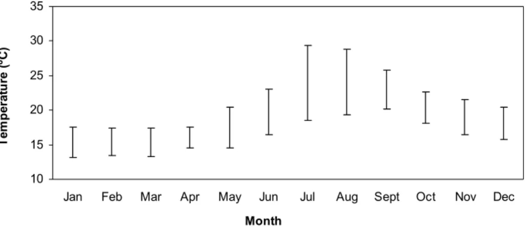
A summary of the location of all in situ temperature measurements described, is presented in Fig.1. Compilation of all these data (Fig. 2) shows that temperature ranges vary during the year, with the highest amplitude observed during summer months and the lowest during winter months. However, some care should be taken when analysing these results since sampling locations vary along the year. The coolest waters (13.2ºC) were observed in January and the warmest (29.4ºC) during July.
10 15 20 25 30 35
Jan Feb Mar Apr May Jun Jul Aug Sept Oct Nov Dec
Month T em p er at u re ( ºC )
AVHRR record characteristics and basic processing
A total of 3331 AVHRR images for the Azores region were obtained from HAZO station from 4th April 2001 to 31st July 2002. Images were processed, using an interactive satellite data analysis software package (TeraScan® 3.1, developed by Seaspace Corporation). FIGUEIREDO et al. (2004) automated all imagery processes, including the use of the MCSST algorithm, with the exception of the navigation that is manual. The resultant cloud-free SST images were remapped to a cylindrical projection occupying a total area from 34º 39.15’ N to 42º 40.30’ N and from 33º 44.08’ W to 23º 30.32’ W. The pixel resolution obtained was 1.1132 x 1.1132 km. From the original 3331 images processed, 53% were rejected mainly due to bad recording and/or coverage, and navigation problems. Maximum temperatures values observed in the images range from 10.2ºC to 32ºC. In situ data (cf. Fig. 2) clearly shows that this temperature range is excessive for the Azores region. The presence of temperature values lower than 13ºC is certainly due to recording and/or atmospheric problems, mainly unresolved clouds that need to be discriminated from the oceanic surface (CAYULA & CORNILLON 1996). To detect the presence and evaluate the frequency of contaminated cloud pixels in the image database, daily SST temperature ranges extracted from the 1575 images obtained, are compared with in situ monthly temperature ranges. Finally, to evaluate the amount and also the impact of these low temperature values on SST average computation, the mean SST value, the mode, the median and the variance of the SST values have been computed on an image-by-image basis.
AVHRR remnant cloud filtering methodologies The most common filtering method consists in eroding (removing) pixels in contact with clouds (CASEY & CORNILLON 1999). A binary erosion that uses a two by two flat structuring element and preserves edges from any erosion (GONZALEZ & WOODS 1992) is tested on the image dataset. The two by two pixel window is superimposed onto the image. Whenever a cloud pixel is
detected within the window area, all the pixels in the image inside the window are changed into cloud pixels. As a result, only the pixels in direct contact with clouds are altered (Fig. 3) even those that are not contaminated, whilst the contamination away from cloud edges is not considered.
Fig. 3. An example of the effect of the erosion filter. Black and white pixels represent clouds and ocean surface, respectively. Ocean surface pixels in contact with clouds are eroded (turn black).
A more selective approach was developed by JONES et al. (1996). Their filtering methodology consists in fitting of a mean, annual, and semi-annual model to the day data, and rejects pixels that differ by more than 3 times the standard deviation of the residuals from this model. This method applies to 2º spatially averaged SST data, except in regions where very few data points are observed.
For the present work the intension was to conserve full resolution images. Also, the amount of data necessary to create an annual model of temperature variability is low. However, this concept (i.e. filtering the images by inputting threshold values as a function of seasonal temperature change) was found to be interesting. In this study, a threshold value was established based on SST data. Then, thresholds were input to each image to remove contaminated pixels before deriving SST composites. In order to obtain representative seasonal temperature changes, 8-consecutive days, rather than daily SST imagery, were used. This allows a better representation of the real temperature range observed within the area under investigation. Thus, temperature histograms were built using 8-consecutive days. If histograms were normally distributed (i.e. if the mean, the median, and the mode of the distribution present close values), extreme values could be removed inputting threshold values. These are equal to the mean distribution plus or minus 3, 4 or 5 times its standard deviation (DANIEL 1987). The coefficient used to define the size of the interval was determined by taking into
consideration the necessity to keep the amount of pixels as large as possible while rejecting contaminated pixels.
By combining SST values from various sensors one can increase the number of data incorporated in the histogram. However, temperature values provided by the different NOAA sensors should be homogeneous. In order to test this, pairs of SST data derived from 2 different sensors (i.e. 12 versus NOAA-14, NOAA-14 versus NOAA-16, and NOAA-12 versus NOAA-16) and recorded within an interval of less than three hours were compared.
A parallel analysis was undertaken to compare, sensor-by-sensor, nighttime and daytime satellite-derived SST data. The difference between day and nighttime SST values of co-located pixels was computed for each pair of images and a total mean difference is obtained. The filtration results were then assessed, first, by comparing satellite-derived SST with co-located in situ data collected in 2001 and 2002 and second, by comparing monthly SST composites before and after running the filter.
Finally, the co-located in situ and satellite data (over the whole data bases) were used to assess the difference in temperature between NOAA-AVHRR and field measurements at daytime (daytime bias) and nighttime (nighttime bias), respectively. Data collected the same day within an interval of less than three hours were considered for comparison.
RESULTS
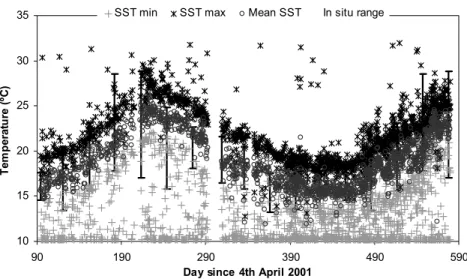
Amount and impact of contaminated pixels Comparison between daily SST temperature ranges extracted from the 1575 images and in situ monthly temperature ranges is displayed in Fig. 4. In general, SST ranges are wider than in situ temperature ones. Nevertheless, with the exception of some high SST values, a fairly good matching seems to exist between maximum SST
and in situ values. On the contrary, SST values lower than 12ºC are found in 50.9 % of the images recorded from spring to autumn. In situ survey values do not show this tendency, which demonstrates that low values, probably linked to unfiltered cloud (CAYULA & CORNILLON 1996), are widely represented in the NOAA database.
However, two tests have been performed to analyse the impact of these low temperature pixels on the average temperature computation. First, the mean and the median are very similar (Table 2), with the latter about 0.05ºC higher than the mean. The mode is generally 0.37ºC lower than the mean. The proximity of the mean, the mode and the median characterises a normal distribution of the SST values in the images. The variance is, on average, 1.45, which means that the SST values are mostly concentrated around the mean, which implies that the impact of cloud-contaminated pixels on the SST value distribution is weak. Second, the determination coefficient between maximum and mean SST values is about 0.79, whilst it decreases down to 0.24 when comparing minimum and mean SST values (Fig. 5).
This low value of the determination coefficient between minimum and mean SST values demonstrates that remnant clouds are recurrent and should be removed to avoid contamination on image composites. Indeed, due to the low number of cloud-free pixels, remnant clouds may appear directly on the resulting composites, or affect pixel-averaged values. Results of these tests suggest that the method proposed to filter the image, based on inputting thresholds determined using the statistical characteristics of the SST distribution, may be particularly adapted to the case studied.
Table 2
Statistics of the SST distribution for the 8-day composites.
Mean (ºC) Median (ºC) Mode (ºC) Variance 18.51 18.56 18.14 1.45
10 15 20 25 30 35 90 190 290 390 490 590
Day since 4th April 2001
T em p erat u re (º C )
SST min SST max Mean SST In situ range
Fig. 4. Comparison between in situ monthly temperature ranges (vertical bars) and AVHRR-derived SST ranges (minimum – crosses, and maximum - stars) as a function of time. The mean SST value computed for each image is represented in circles. y = 0,5824x + 2,2258 R2 = 0,2617 y = 0,9707x + 3,5458 R2 = 0,7654 0 5 10 15 20 25 30 35 10 12 14 16 18 20 22 24 26 28 Mean SST (ºC) SST ( ºC ) SST min SST max
Fig. 5. Regression between minimum (circles) and mean and maximum (crosses) and mean SST values, respectively, derived on an image-by-image basis.
Inter-sensor comparison
All NOAA sensors are initially used for inter-sensor comparison. NOAA-14 images can only occasionally be compared with NOAA-16, because the record time lag between these sensors is generally more than 3 hours. Results show that the mean difference between NOAA-12 and NOAA-16 is negligible whilst NOAA-12 is
negatively biased by about 0.24ºC in comparison to 14 (Table 3). Although this NOAA-12/NOAA-14 difference is lower than general NOAA sensors measurement accuracy, it is important to notice that this difference is observed over the whole investigated period. The mean time interval between the two sensor measurements is generally low (45’) and cannot explain this difference.
Table 3
Comparison of SST values recorded by NOAA-12, -14 and -16.
Sensor
name difference (ºC) Mean SST Standard deviation overlaid images Number of overlaid pixels Number of
NOAA-12 NOAA-14 -0.24 0.33 67 2,437,385 NOAA-12 NOAA-16 0.06 0.5 163 2,951,101 NOAA-14 NOAA-16 -0.05 0.17 4 92,916
The high values observed for the mean standard deviation (cf. Table 3) are probably related to the comparison between oceanic SST and low value (cloud influenced) pixels. In fact, SST differences greater than 5ºC are found in 27% of the studied cases, which is considerable and shows the impact of cloud-contaminated pixels on this test. To conclude, the proximity of the SST values obtained from the different sensors shows that all sensors can be merged for further processing and analysis.
Daytime and nighttime comparison
A total of 1008 and 567 images were recorded at daytime and nighttime, respectively. Overlaid valid pixels were found in 433 pairs of images. Within all pairs, a total of about 3 millions of pixels were found valid for comparison. Using this entire set of data, the mean SST difference between daytime and nighttime is about 0.9ºC. However, this value changes along the year (Table 4).
Table 4
Mean SST difference (ºC) between daytime and nighttime dataset
Month daytime and nighttime SST Mean difference between
January 0.16 ± 0.69 February 0.48 ± 1.02 March 0.35 ± 0.58 April 1.30 ± 1.03 May 0.99 ± 0.77 June 1.02 ± 0.73 July 1.20 ± 0.63 August 0.91 ± 1.22 September 0.68 ± 1.42 October 0.13 ± 1.36 November 0.18 ± 1.63 December 0.22 ± 1.31
From February to September, the bias between daytime and nighttime SST is higher
than the accuracy obtained by deriving SST values from satellite measurements. Therefore, the February to September daytime and nighttime SST data should be analysed separately. On the contrary, from October to January, this bias is lower than the SST measurement accuracy but it exhibits a large standard deviation (cf. Table 4). These low biases mean that, at least from October to January, sea surface temperature variations between night and day are reduced. This is mainly due to the lowest insulation and highest wind speeds that characterize autumn and winter in this region (BETTENCOURT 1979), both tending to decrease the sea surface warming (STRAMMA et al. 1986). Therefore, it seems possible to merge nighttime and daytime data recorded from October to January. However, these biases present strong variations as reflected by the high standard deviations values obtained. This is probably caused by the presence of remnant clouds and/or variable wind speed. This implies that before combining daytime with nighttime imagery, each night/day couple should be examined to prove that temperature values do not change significantly during the 24 h considered. Evaluation of the filters
Filtering by erosion. Eroding systematically all
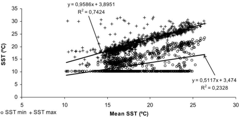
pixels in contact with clouds removes about 34% of the initial cloud-free pixels, which drastically decreases the amount of available pixels for analysis, particularly during the winter months, where after erosion, less than 5% of the pixels in the images represent the water surface. A study of the SST values of the eroded images demonstrates the coarse performances of this filter. Erosion is able to clear about one half of the very high SST values. Finally, after running the erosion filter, images from spring, summer, and autumn still present about 38% of SST values lower than 12ºC. In fact, when comparing minimum and mean SST values, the determination coefficient (Fig. 6) remains as low as when performing this comparison before eroding the images (cf. Fig. 5). This signifies that the erosion filter, although removing subpixel clouds present at the edges of cloudy areas, only extracts a small part of the pixels presenting SST values strongly affected by cloud contamination.
y = 0,5117x + 3,474 R2 = 0,2328 y = 0,9586x + 3,8951 R2 = 0,7424 0 5 10 15 20 25 30 35 5 10 15 20 25 30 Mean SST (ºC) SST ( ºC ) SST min SST max
Fig. 6. Regression between minimum (circles) and mean and maximum (crosses) and mean SST values, respectively, derived on an image-by-image basis, after applying the erosion filter.
Filtering by histogram thresholding. The number
of images recorded during 8 consecutive days at daytime and nighttime ranges from 1 to 40 (with a mean rate of 17) and from 2 to 20 images (with a mean rate of 10 images), respectively. The 8-day SST values show a normal distribution as demonstrated by the proximity of the mean, the median, and the mode of the respective histogram distributions. On average, the mean is about 0.04ºC lower than the median, and about 0.4ºC higher than the mode (Table 5). The standard deviation is, on average, 1.43, which means that the SST values are mostly concentrated around the mean.
Table 5
Statistics of the SST distribution for the 8-day composites, after inputting thresholds.
Mean (ºC) Median (ºC) Mode (ºC) Variance 18.54 18.58 18.14 1.43 Information of in situ monthly temperature ranges with SST-derived maximum and minimum ranges is shown in Fig. 7. The threshold values, deduced from the 8-day SST imagery distributions, are also presented for comparison. These are obtained by calculating the mean of the distributions plus or minus 3, 4, and 5 times their
standard deviation (STD). This comparison shows that the broader filter (5 times STD) allows SST values below 10ºC to pass, whilst cutting the range at 3 times STD removes, in some cases, in
situ measured values. Furthermore (cf. Fig. 4), the
satellite derived-SST range exceeds in several cases the one measured in situ. Therefore, a 3 times STD filter may significantly reduce the satellite derived SST ranges. Taken this into consideration, a 4 times STD filter seems to be appropriate to characterise minimum and maximum SST data for the Azores region and for this particular data set.
A particular problem found with this methodology is that, in some cases, the computed threshold values vary by more than 2ºC from one week to the next (cf. Fig. 7) because consecutive weeks can present rapid fluctuations on the total amount of valid images. To remove this variability, the threshold series are smoothed using a window with a width of 2.
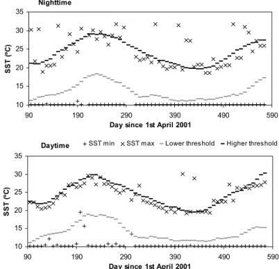
The superimposition of the 8-day smoothed thresholds to the SST-derived minimum and maximum values obtained from the 8-day composites (Fig. 8) shows that low and high temperature values were removed in the majority of the cases.
0 5 10 15 20 25 30 35 40 90 190 290 390 490 590
Julian day (since 1st April 2001)
T em p er at u re ( ºC )
Mean +/- 3SD Mean +/- 4 SD Mean +/- 5SD Min SST Max SST
Fig. 7. Comparison of in situ monthly temperature ranges (vertical bars) with 8-day SST-derived maximum (crosses), minimum (stars), and threshold values. Thresholds are equal to the mean of the distributions plus or minus 3, 4, and 5 times their standard deviation (STD), respectively.
Nighttime 10 15 20 25 30 35 90 190 290 390 490 590
Day since 1st April 2001
SS T ( ºC ) Daytime 10 15 20 25 30 35 90 190 290 390 490 590
Day since 1st April 2001
SST
(
ºC
)
SST min SST max Lower threshold Higher threshold
Fig. 8. Comparison of the 8-day smoothed thresholds to the SST-derived minimum (crosses) and maximum (x) values obtained from the 8-day composites.
On an image-by-image case, nighttime threshold values remove from 0 to 96% of the pixels with an average rate of 2%. Daytime threshold values remove from 0 to 70% of the
pixels with a mean rate of 1%. These averages are very low, in part due to the fact that in 101 nighttime cases and 557 daytime cases, no pixels were removed. Finally, only 3.6% of the pixels
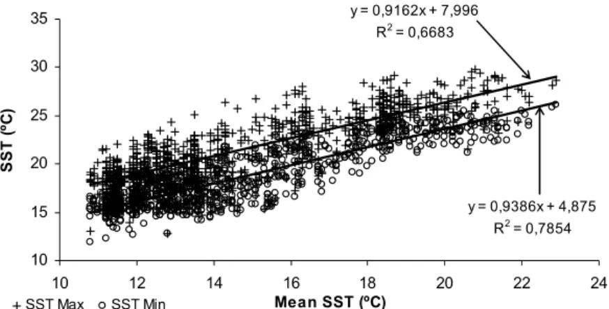
with SST values lower than 12ºC are found from spring to autumn. As it was previously done before filtering the images and after running the erosion filter (cf. Fig. 5 and Fig. 6), the mean SST value for each image has been plotted in function of corresponding minimum and maximum SST values obtained after inputting thresholds (Fig. 9).
In this case, both regressions present high determination coefficients. This demonstrates the efficiency of the implemented filter. An example of the effect of the threshold filter in a monthly average SST image is presented in Fig. 10. Low pixel values (north/northeast of the Azores) are successfully removed. y = 0,9162x + 7,996 R2 = 0,6683 y = 0,9386x + 4,875 R2 = 0,7854 10 15 20 25 30 35 10 12 14 16 18 20 22 24 Mean SST (ºC) SST ( ºC ) SST Max SST Min
Fig. 9. Regression between minimum (circles) and mean and maximum (crosses) and mean SST values, respectively, derived on an image-by-image basis, after inputting thresholds to the images.
Fig. 10. An example of the effect of the threshold filter on an average SST image obtained in July 2001. The filtered image is displayed on the right hand side. Nighttime (nn) composites resulting from the merging of NOAA-12, -14 and –16 imagery (ALL) are displayed.
Comparison of satellite-derived SST with in situ data
Concurrent surface and 3 m depth temperature in
situ data show high correlation (Fig. 11). On
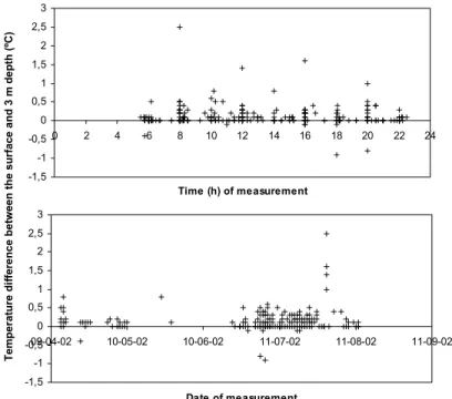
average, surface temperatures are 0.12ºC higher than those collected at 3 m depth (with a variance of 0.07ºC) and apparently, there is no relation between the time or date of sampling and the
difference between surface and 3 m water temperature (Fig. 12). This suggests that the first metres of the water column are poorly stratified from April to August (i.e. at the time the in situ measurements have been carried out). These results imply that water temperatures measured at least, down to 3 m depth, can be safely compared with satellite-derived SST data.
y = 1,0005x - 0,1325 R2 = 0,9857 14 16 18 20 22 24 26 14 16 18 20 22 24 26 Temperature at 0.5 m depth (ºC) Te m p er at ur e a t 3 m de pt h ( ºC )
Fig. 11. Correlation between calibrated in situ measurements carried out at about 50 cm below the water surface and at 3 m depth. -1,5 -1 -0,5 0 0,5 1 1,5 2 2,5 3 0 2 4 6 8 10 12 14 16 18 20 22 24 Time (h) of measurement -1,5 -1 -0,5 0 0,5 1 1,5 2 2,5 3 09-04-02 10-05-02 10-06-02 11-07-02 11-08-02 11-09-02 Date of measurement
Fig. 12. Temperature difference between in situ surface and 3 m depth as a function of time (top) or date (bottom) of sampling. Temper ature d if fe re n c e bet w een t h e surf ac e a n d 3 m d e p th ( ºC)
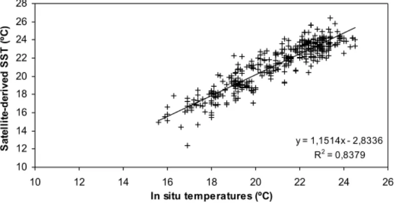
Amongst the 3318 in situ measurements available for comparison with SST data, 402 matched single non-cloud pixels (394 corresponding to daytime paths and 8 to nighttime paths). The determination coefficient obtained from the comparison between in situ and satellite data is 0.84, with satellite positive bias of 0.34ºC and scatter (i.e. standard deviation of the
difference between in situ and remotely sensed temperatures) of about 1.1ºC (Fig. 13). At nighttime negative biases of 0.74ºC are observed. Over the whole year, daytime biases are positive (0.36ºC) and present important fluctuations with season. SST values are positively biased by 0.61ºC during the summer and negatively biased by -0.41ºC during the spring.
y = 1,1514x - 2,8336 R2 = 0,8379 10 12 14 16 18 20 22 24 26 28 10 12 14 16 18 20 22 24 26 In situ temperatures (ºC) Sa te llit e-d er iv ed SST ( ºC )
Fig. 13. Comparison between co-located in situ and satellite-derived temperature values. Measurements carried out at daytime have been considered.
DISCUSSION
The biases observed between satellite and in situ measurements are explained by the fact that thermal sensors determine the temperature of the “skin” of the ocean, a molecular boundary layer less than 1 mm thick that is responsible for heat flux between the ocean and the atmosphere (skin effect, SHLUESSEL et al. 1987). The “bulk” ocean temperature is obtained in the field. Because the net flux is generally towards the atmosphere the “skin” is generally cooler than the “bulk” temperature. At daytime, the sea surface is warmed by solar insulation, and the effect of this diurnal warming (STRAMMA et al. 1986) is increased in low wind conditions (CASEY 2002; GENTEMANN et al. 2003) by leading to positive bias day. In the case of the Azores, a negative bias is found at night, and by day during spring, whilst positive bias is found by day during summer months. In fact, winds appear stronger during the spring than during the summer (BETTENCOURT 1979), which explains why daytime bias is negative in spring and positive in summer. As shown by the dataset presented in
this contribution, CASEY (2002) recently demonstrated that daytime bias is lower than nighttime bias, for about 5000 co-localised observations, whilst the contrary was generally admitted (WELLINGTON et al. 2001). However, CASEY (2002) also suggests that daily variations in space and time are more important than those observed during the night.
Therefore, comparison between satellite and
in situ data proves that NOAA-12, -14 and -16
SST, imageries are well adapted to study meso-scale oceanographic features in the Azores. However, the accuracy of the remnant cloud filtering scheme implemented in this study requires further discussion. Undetermined clouds are one of the major sources of errors in determining SSTs accurately (JONES et al. 1996). This study shows that cloud contamination is located mainly away from cloud edges. Sensors with increased spectral information and spatial resolution, like MODIS (Moderate Resolution Imaging Spectroradiometer), remove cloud-contaminated pixels at a higher rate (HEIDINGER et al. 2002). In addition, other satellites such as the MSG-geostationary EUMETSAT, could
provide superior ability in removing noise by clouds through its higher temporal frequency capacity. Also, marine low stratiform clouds, such as fog, stratus, and stratocumulus are very difficult to differentiate from seawater, and may be detected by cluster analysis (SIMPSON et al. 2001). The automated thresholding method implemented in this work is simple as it uses directly the SST values determined in each image and builds SST value histogram distributions over 8-day images. However, resulting histograms also represent cloud-contaminated pixels.
The impact of erroneous pixels on SST average computation is assessed comparing mean SST in each image before and after histogram thresholding. This comparison (cf. Table 2 and Table 5) shows that mean SST values are 4x10⁻²ºC higher after filtering. As SST values are
rounded off to one decimal place, the impact of mean SST underestimation on threshold computation is insignificant.
Results show that SST-derived NOAA-14 values are positively biased by about 0.24ºC when compared with SST-derived NOAA-12 and NOAA-16 records. As the origin of this bias may be, at least partially, attributed to the comparison between cloud-free pixels and pixels presenting remnant clouds, the difference between SST-derived NOAA-12 and SST-SST-derived NOAA-14 values were computed after image thresholding. It appears that this test does not allow a positive bias of NOAA-14. This bias probably result from trends and uncertainties in thermal calibration of AVHRR radiometres that vary with the channels and sensor type, and impact the retrieval of the temperature by more than 0.1 K (TRISHCHENKO et al. 2002). Therefore, NOAA-14 may be either removed or corrected to perform more accurately average computations. In the first case, removal of the NOAA-14 images seems to affect the determination of the threshold values used in image filtering. In fact, the mean value of the histogram remains approximately the same but the standard deviation is significantly increased at daytime, which means that the filter is less able to remove remnant clouds. The effect at nighttime is less due to the lower number of NOAA-14 images recorded at night. At nighttime, the removal of NOAA-14 imagery affects only the overall average computation. These results
suggest that SST-derived NOAA-14 images should rather be corrected than removed. Hence, all available SST images should be used in 8-day temperature histogram building.
The mean value of the daytime/daytime bias (0.76ºC) is much larger than those found in the literature (WELLINGTON et al. 2001; CASEY 2002). This is probably related to the small size and the spatial and time inconsistency of the database used for the comparison. The change from spring negative to summer positive biases may be due to a decrease of wind activity from spring to summer (BETTENCOURT 1979) with an increase in skin layer warming (STRAMMA et al. 1986). In the Azores the winds are globally strong but present a large day-to-day variability. Hence, daytime bias variation may be important. Then, even if nighttime data present on average a more important negative bias (CASEY 2002), these are less subjected to day-to-day changes and are therefore, more easily exploitable for studying the climatology of the Azores.
In summertime, this filter is very efficient, but during the winter, the same low temperature values may represent low stratiform clouds and/or water pixels. In winter, threshold values may be as low as 10.5ºC. However, around the Azores islands it is shown that sea surface temperatures are generally higher than 12ºC. Lower temperatures may be found further north. Therefore, it may be interesting during the winter to determine threshold values according to various latitude ranges. However, the number of pixels is reduced in winter, and therefore threshold values may be difficult to determine with precision. Further experiments should be made to demonstrate that in some cases, nighttime and daytime images may be used together to carry out 8-day histograms and to define accurate SST thresholds.
The filtering method presented in this study is more powerful than the erosion method to remove pixels noticeably affected by clouds. However, the erosion method has the advantage of removing pixels in contact with clouds that may include only a small percentage of cloud cover. However, the erosion should be avoided in the Azores region, where cloud cover is frequent, since this method removes a large amount of pixels, reducing the possibility to obtain good and
repetitive SST coverage, particularly during wintertime. More generally, the erosion presents the following disadvantages. First, it may remove non-contaminated pixels, reducing the already low amount of pixels available for further investigation. Second, erosion cannot filter out cloud contaminated SST pixels located away from cloud edges, which may decrease the accuracy of SST composites. In the future, retrieval of SST values can be improved, by implementing additional filters after image thresholding. This filter implementation should involve two other steps. First, the temperature variability among adjacent pixels must be calculated. Second, an evaluation of the risk for a pixel to be contaminated by neighbouring cloud must be addressed.
The histogram thresholding technique, seems appropriate for the Azores region. However, this technique should not be used in regions where strong natural temperature variation occurs (e.g. intensive upwelling areas).
CONCLUSIONS
This study presents the first insight in NOAA-AVHRR imagery received by the HAZO HRTP receiving station located in the Azores, and contributes to provide SST data with higher level of accuracy. The Azores region shows very high cloud contamination. It is essential to obtain good quality satellite data in order to describe temporal and spatial distribution of sea surface temperature in complex regions such as the Azores. With this objective, a new method that removes bad pixel values mainly linked to the presence of numerous undetected clouds was developed. The method is based on inputting thresholds on images. Threshold values are defined using the mean of 8-day SST histograms plus or minus 4 times their standard deviation. Results suggest that daytime and nighttime histograms must be differentiated, and that all NOAA sensors data can be merged, regardless the SST NOAA-14 general overestimation. This filtering scheme seems to be well adapted to the Azores region, since, from spring to autumn, it removes almost 97% of erroneous pixels. The accuracy of this method in determining cloud influence at cloud edge, and in
removing erroneous pixels in wintertime has been discussed and some improvements were made. The comparison between co-located in situ temperatures and AVHRR-derived SST values shows that remotely sensed data are positively biased by 0.34ºC with a mean scatter of 1.1ºC. The bias is within the range expected (CASEY 2002) but the scatter may be reduced by implementing nonlinear sea surface temperature algorithms (WALTON et al. 1998). Nevertheless, results are encouraging since SST average-derived all sensors nighttime values describe accurately water structures (e.g. anomalies) and SST-derived skin layer data provide upper mixed layer information. Further investigation regarding SST distribution in the Azores is proposed as a second part of this paper. The latter also discusses the influence of the North Atlantic Oscillation on SST variability. Finally, since overlaying physical oceanographic and fishery data involves potential applications in fisheries monitoring (ANDRADE & GARCIA 1999; COLE & VILLACASTIN 2000; WALUDA et al. 2001), improving the knowledge on meso-scale circulation in the Azores using satellite data will help to understand the decrease of catches observed for several pelagic and demersal species in these last few years (KRUG 1994; PEREIRA 1995; PINHO 2002).
ACKNOWLEDGEMENTS
We would like to sincerely thank all the team members at the Oceanography Section at the Department of Oceanography and Fisheries at the University of the Azores (DOP/UAç). In particular, we thank Paola Castellanos for her invaluable help during HAZO installation and first steps of imagery processing.
For assistance in in situ temperature sampling we gratefully acknowledged the captain, crew, and scientific staff of R/V ARQUIPÉLAGO cruises “ARQDAÇO-02” (MAREDA project – Annual monitoring of the relative abundance of demersal species of the Azores) and “VENTOX” (Deep-Sea Hydrothermal Vents: A Natural Pollution Laboratory) (EVK3CT1999-00003); Rogério Feio, responsible for the coordination of the program POPA (Program for the Observation
of Fisheries of the Azores); and to all the observers on board the Azorean tuna fleet as part of POPA cruises.
Computer resources and facilities were provided by DOP/UAç and by the Institute of Meteorology (Azores). This work was supported by the following: project DETRA, funded by the Regional Directorate of Fisheries of the Azores (RAA - SRAPA / DRP - DETRA - 2000 - 2003), Centre of IMAR (Instituto do Mar) of the University of the Azores funds, and the Foundation for Science and Technology (Ministry of Science and Technology of Portugal) through a Post-Doctorate Fellowship. This support is greatly acknowledged.
REFERENCES
ALVES,M.L.G.R.&A.C. DE VERDIERE 1999.Instability dynamics of a subtropical jet and applications to the Azores front current system: Eddy-driven mean plow. Journal of Physical Oceanography 29(5): 837-864.
ANDRADE, H.A. & C.A.E. GARCIA 1999. Skipjack tuna
fishery in relation to sea surface temperature off the southern Brazilian coast. Fisheries Oceanography 8(4): 245-254.
BETTENCOURT, M.L. 1979. O clima dos Açores como
recurso natural, especialmente em agricultura e indústria de turismo. O Clima de Portugal, 18, INMG, Lisboa.
CASEY, K.S. 2002. Daytime vs nighttime AVHRR sea surface temperature data: a report regarding Wellington et al. (2001). Bulletin of Marine Science 70(1): 169-175.
CASEY, K.S. & P. CORNILLON 1999. A comparison of
satellite and in situ-based sea surface temperature climatologies. Journal of Climate 12: 1848-1862. CAYULA, J.F. & P. CORNILLON 1996. Cloud Detection
from a sequence of SST images. Remote Sensing of Environment 55:80-88.
CIPOLLINI, P., D. CROMWELL, M.S. JONES, G.D.
QUARTLY & P.G. CHALLENOR 1997. Concurrent
altimeter and infrared observations of Rossby wave propagation near 34° N in the Northeast Atlantic. Geophysical Research Letters 24(8): 889-892. COLE, J. & C. VILLACASTIN 2000. Sea surface
temperature variability in the northern Benguela upwelling system, and implications for fisheries research. International Journal of Remote Sensing 21(8): 1592-1617.
CROMWELL D., P.G. CHALLENOR, A.L. NEW & P.D.
PINGREE 1996. Persistent westward flow in the
Azores Current as seen from altimetry and hydrography. Journal of Geophysical Research, 101(C5): 11923-11933.
DANIEL, W.W. 1987. Biostatistics: A foundation for
Analysis in the Health Sciences. Fourth Edition, Wiley Series in Probability and Mathematical Statistics-Applied. John Wiley and Sons, Inc., 734 pp.
DONLON, C.J., S.L. CASTRO &A. KAYE 1999. Aircraft
validation of ERS-1 ATSR and NOAA-14 AVHRR sea surface temperature measurements. International Journal of Remote Sensing 20(18): 3503-3513.
EFTHYMIADIS, D., F. HERNANDEZ & P.Y.LE TRAON
2002. Large-scale sea-level variations and associated atmospheric forcing in the subtropical north-east Atlantic Ocean. Deep-Sea Research Part II 49(19): 3957-3981.
FIGUEIREDO, M., P. CASTELLANOS, A. MARTINS, A.
MENDONÇA, L. MACEDO, M. MELO RODRIGUES, V. LAFON &N. GOULART. 2004. A software package for automated AVHRR and SeaWiFS acquisition and processing. Interim progress report. Arquivos do DOP. Série Relatórios Interno, no. 3/2004: 89 pp.
GENTEMANN,C.L.,C.J.DONLON,A.STUART-MENTETH
&F.J.WENTZ 2003. Diurnal signals in satellite sea
surface temperature measurements. Geophysical Research Letters 30: Art. No. 1140.
GONZALEZ, R. & R. WOODS 1992. Digital Image
Processing, Addison-Wesley Publishing Company. 716 pp.
GOULD, W.J. 1985. Physical oceanography of the Azores front. Progress in Oceanography 14: 167-190.
HEIDINGER A.K., V.R. ANNE &C. DEAN 2002. Using MODIS to estimate cloud contamination of the AVHRR data record. Journal of Atmospheric and Oceanic Technology 19(5): 586-601.
JONES, M.S., M.A. SAUNDERS & T.H. GUYMER 1996.
Global remnant cloud contamination in the along-track scanning radiometer data: Source and removal. Journal of Geophysical Research 101(C5): 12,141-12,147.
KABBARA,N.,X.H.YAN,V.V.KLEMAS &J.PAN 2002.
Temporal and spatial variability of the surface temperature anomaly in the Levantine Basin of the Eastern Mediterranean. International Journal of Remote Sensing 23(18): 3745-3761.
KIELMANN, J., & R.H. KASSE 1987. Numerical
modelling of meander and eddy formation in the Azores Current frontal zone. Journal of Physical Oceanography, 17: 529-541
KLEIN, B. & G. SIEDLER. 1989. On the origin of the
Azores Current. Journal of Geophysical Research 94: 6159-6168.
KRUG, H. 1994. Biologia e avaliação do stock açoriano
de goraz, Pagellus bogaraveo. PhD thesis. Department of Oceanography and Fisheries, University of the Azores, Horta. Arquivos do DOP, Série estudos, No.7/94. 192 pp.
LE TRAON, P.Y.&P.DE MEY 1994. The eddy field associated with the Azores front east of the Mid-Atlantic Ridge as observed by the GEOSAT altimeter. Journal of Geophysical Research 99(C5): 9907-9923.
LAFON,V.,A.MARTINS,I.BASHMACHNIKOV,M.MELO -RODRIGUES & M. FIGUEIREDO 2003. Sea surface temperature spatio-temporal variability in the Azores using a new technique to remove invalid pixels. Pp.: 89-97 in: BOSTATER, C.R. JR. & R.
Santoceri (Eds). Remote Sensing of Ocean and Sea Ice, Proceedings of SPIE Vol. 5233, 394 pp. MAILLARD, C. 1986. Atlas hydrologique de l'Atlantique
nord-est. IFREMER: Brest, France. 133 pp. MCCLAIN, E.P., W.G. PICHEL & C.C. WALTON 1985.
Comparative performance AVHRR-based multichannel sea surface temperatures. Journal of Geophysical Research 90: 11,587-11,601. PEREIRA, J.G. 1995. A pesca do atum nos Açores e o
atum patudo (Thunnus obesus, Lowe 1839) do Atlântico. Arquivos do DOP. Série Estudos, n.º 1/95: 330 pp.
PICHEL W.G. 1991. Operational production of
Multichannel Sea-Surface Temperatures from NOAA polar satellite AVHRR data. Global Planet Change 90(1-3): 173-177.
PINGREE, R. 1997. The eastern subtropical gyre (North
Atlantic): Flow rings recirculations structure and subduction. Journal of the Marine Biological Association of the UK 77: 573-624.
PINGREE, R. 2002. Ocean structure and climate (Eastern
North Atlantic): in situ measurement and remote sensing (altimeter). Journal of the Marine Biological Association of the UK 82: 681-707. PINGREE, R.D., C. GARCIA-SOTO & B. SINHA 1999.
Position and structure of the Subtropical/Azores front region from combined Lagrangian and remote sensing (IR/altimeter/SeaWiFS) measurements. Journal of the Marine Biological Association of the UK 79: 769-792.
PINGREE, R., Y.-H. KUO &C. GARCIA-SOTO 2002. Can the subtropical North Atlantic permanent thermocline be observed from space? Journal of Marine Biological Association of the UK, 82: 709-728.
PINGREE, R.& B.SINHA 1998.Dynamic topography
(ERS-1/2 and seatruth) of subtropical ring
(STORM 0) in the storm corridor (32-34 degrees N, eastern basin, North Atlantic Ocean). Journal of Marine Biological Association of the UK 78(2): 351-376.
PINGREE,R.&B.SINHA 2001. Westward moving waves
or eddies (Storms) on the Subtropical/ Azores Front near 32.5 degrees N? Interpretation of the Eulerian currents and temperature records at moorings 155 (35.5 degrees W) and 156 (34.4 degrees W). Journal of Marine System 29(1-4): 239-276. PINHO, M.R. 2002. Abundance estimation and
management of Azorean demersal species. PhD thesis. Department of Oceanography and Fisheries, University of the Azores, Horta, 163 pp.
POLLARD, R.T. & S. PU 1985. Structure and Circulation of the upper Atlantic ocean Northeast of the Azores. Progress in Oceanography 14: 443-462. REVERDIN,G.&F.HERNANDEZ 2001.Variability of the
Azores Current during October-December 1993. Journal of Marine Systems 29(1-4): 101-123. REYNOLDS, R.W., N.A. RAYNER, T.M. SMITH, D.C.
STOKES &W.Q.WANG 2002. An improved in situ and satellite SST analysis for climate. Journal of Climate 15(13): 1609-1625.
SCHUESSEL,P., H.-Y.SHIN, W.EMERY &H.GRASSL
1987. Comparison of satellite derived sea suface temperature with in situ skin measurements. Journal of Geophysical Research 92: 2859-2874. SIMPSON, J.J. & C.HUMPHREY 1990. An automated
cloud screening algorithm for daytime AVHRR imagery. Journal of Geophysical Research, 95: 13457-13458.
SIMPSON J.J., T.J. MCINTIRE, J.R. STITT & G.L.
HUFFORD 2001. Improved cloud detection in
AVHRR daytime and night-time scenes over the ocean. International Journal of Remote Sensing 22(13): 2585-2615.
STRAMMA, L., P. CORNILLON, R.A. WELLER, J.F. PRICE
& M.G. BRISCOE 1986. Large diurnal sea surface
temperature variability: Satellite and in situ measurements. Journal of Physical Oceanography 16: 827-837.
TEJERA, A., L. GARCIA-WEIL, K.J. HEYWOOD & M.
CANTON-GARBIN 2002. Observations of oceanic
mesoscale features and variability in the Canary Islands area from ERS-1 altimeter data, satellite infrared imagery and hydrographic measurements. International Journal of Remote Sensing 23(22): 4897-4916.
TRISHCHENKO, A.P., G. FEDOSEJEVS, Z. LI & J. CIHLAR
2002. Trends and uncertainties in thermal calibration of AVHRR radiometres onboard NOAA-9 to NOAA-16. Journal of Geophysical Research 107(D24): 4778.
VARGAS, J.M., J. GARCIA-LAFUENTE, J. DELGADO & F.
CRIADO 2003. Seasonal and wind-induced
variability of sea surface temperature patterns in the Gulf of Cadiz. Journal of Marine Systems 38(3-4): 205-219.
WALUDA, C.M., P.G. RODHOUSE, P.N. TRATHAN & G.J. PIERCE 2001. Remotely sensed mesoscale
oceanography and the distribution of Illex argentinus in the South Atlantic. Fisheries Oceanography 10(2): 207-216.
WALTON, C.C., W.G. PICHEL, J.F. SAPPER & D.A. MAY
1998. The development and operational application of nonlinear algorithms for the measurement of sea surface temperatures with the NOAA
polar-orbitong environmental satellites. Journal of Geophysical Research, 103(C12): 27,999-28,012. WEEKS,S.J.,F.A.SHILLINGTON &G.B.BRUNDRIT 1998.
Seasonal and spatial SST variability in the Agulhas retroflection and Agulhas return current. Deep-Sea Reasearch Part I 45(10): 1611-1625.
WELLINGTON, G.M., A.E. STRONG &G. MERLEN 2001. Sea surface temperature variation in the Galápagos Archipelago: a comparison between AVHRR nighttime satellite sata and in situ intrumentation (1982-1998). Bulletin of Marine Science 61(1): 27-42.