doi: 10.5540/tema.2018.019.03.0509
A Trajectory Planning Model for
the Manipulation of Particles in Microfluidics
L. MEACCI, F.F. ROCHA, A.A. SILVA, P.V. PRAMIU and G.C. BUSCAGLIA
Received on October 03, 2017 / Accepted on May 30, 2018
ABSTRACT. Many important microfluidic applications require the control and transport of particles im-mersed in a fluid. We propose a model for automatically planning good trajectories from an arbitrary point to a target in the presence of obstacles. It can be used for the manipulation of particles using actuators of me-chanical or electrical type. We present the mathematical formulation of the model and a numerical method based on the optimization of travel time through the Bellman’s principle. The implementation is focused on square grids such as those built from pixelated images. Numerical simulations show that the trajectory tree produced by the algorithm successfully avoids obstacles and stagnant regions of the fluid domain.
Keywords: Trajectory planning, manipulation of particles in microfluidics, Bellman’s principle.
1 INTRODUCTION
Particle manipulation is an important topic in microfluidics, a science that studies the behavior of small-scale fluids. A growing interest exists in the steering of particles in microfluidic systems, especially in the biological and medical fields, to analize elements of very small size such as proteins or DNA. In particular, improving the ability to manipulate and to steer particles in mi-crofluidics can allow to better examine, control and treat biological materials. Some interesting examples are the microfluidic device presented in [13] or the use of optical tweezers as tools to move in a controlled way individual particles, as shown in [6].
The control of the trajectory of particles immersed in a fluid by boundary actuators is the topic presented in the articles by Chaudhary and Shapiro [4] and Tuval et. al. [12]. The microfluidic modeling in these works proposes the displacement of the particles from one point to another by a pre-established trajectory. The idea is to identify the location of the particle in real time so that a control algorithm calculates the demand on each actuator for the flow to carry the particle along the desired path. In Armani et. al., [1] and [2], some examples can be found of the use of control
*Corresponding author: Luca Meacci – E-mail: [email protected]
techniques. A generalization for the manipulation of particles in the three-dimensional case also exists in the study of Probst and Shapiro [10].
In all published methods discussed above, a predefined trajectory is necessary as a datum but no mention is given about how to build such a trajectory. In fact, in their examples the trajectory is introduced manually. The present work proposes a method to automatically define a “good” tra-jectoryγ∗that can then be used as input for those particle manipulation techniques. By “good” we intend thatγ∗not only avoids obstacles, but also avoids parts of the fluid domain where the
actu-ators are ineffective at producing flow (stagnant regions, or regions of low controllability). These requirements are fulfilled by time-optimal trajectories, which are the ones proposed here. In fact, we propose an algorithm that works on a rectangular grid and could be implemented directly on a pixelated image of the domain. The trajectories are discrete in the sense that they are broken lines joining neighbor grid points. This is a very practical, though not smooth, parameterization of possible paths. The resulting trajectoryγ∗can eventually be smoothed out before passing it to the manipulation algorithm. The combination of the proposed method with the manipulation techniques of Shapiro and coworkers ([4], [1], [2] and [10]) would allow for an integrated system of detection, planned manipulation and control of particles towards an arbitrary target.
The presentation begins by describing the general physical model and recalling the techniques used for particle steering when the desired trajectory is known. This allows us to introduce several concepts needed for trajectory planning. Then the continuous problem of optimizing trajectories (Bellman’s principle) with respect to arrival time is described, together with the proposed dis-cretization. Finally, applications are reported in the section of numerical results. They show the good performance of the algorithm in finding suitable, sometimes counterintuitive, trajectories.
2 THE PHYSICAL MODEL
We study the manipulation of a particle in a microfluidic device in the two-dimensional case, the extension to 3D being immediate. In fact, we can see the 2D case applicable to flows between flat plates parallel to the planexy, in the case when the plates are sufficiently close.
Let us consider therefore a square domain(0,L)2=Ω, for the flow of a fluid without inertia
with the presence of obstacles, walls and also of actuators. As we can see in the Figure 1, the actuators act in some regions of the boundary of the domainΓN,ΓS,ΓEandΓW, being placed on the respective north, south, east and west borders.
At each actuator we apply a valueXN,XS,XE eXW. Since the driving force of the flow is the difference between actuator values (pressure or electrical potential differences), we can fixXE
to zero without losing generality and work only with the variablesX= (XN,XS,XW)T. Inertial effects are generally negligible in microfluidics. As a consequence, eachX∈A (whereA is
the set of admissible actuator values) leads to a velocity field according to the following linear relation
S
W E
N
Obstacle Wall
Wall
Figure 1: Sketch of the domain configuration.
The matrixB(~x) = (BN(~x),BS(~x),BW(~x))T contains as columns the components of the velocity field at the point~xwithX belonging to the canonical basis, i.e.XN =1,XS=0 andXW =0 for the first column;XN=0,XS=1 andXW=1 for the second one andXN=0,XS=0 andXW=1 for the third one. The Figure 2 shows an example of the velocity field, for some points of the domain, generated by imposing the canonical basis.
Figure 2: Velocity fields generated by imposing the canonical basis. All possible velocity fields are linear combinations of these three.
The admissible set of the controlsA generates an admissible set of velocitiesV(~x)on each point, defined by
V(~x) ={~w∈Ω| ∃X ∈A ,~w=B(~x)X}.
LetPbe a passive point particle whose initial position is~x0. Each control functionX(t):[0,T]→
A movesPalong a trajectory~r(t)that is the solution of the following problem
( d~r
dt =~v(~r(t),X(t)) ~r(0) =~x0.
The goal of this work is to answer the question of how to determine the control functionX∗(t) that moves the particlePfrom the position~x0to a target setZ⊂Ω. The target setZmay be a region of the domain where the particle is analyzed or subjected to some biochemical reaction, for example. In order to completely achieve this aim we have first to solve the problem of the particle manipulation through a predefined path. As explained in the following subsection, this approach introduces an optimization problem for maximizing the possible velocity. The solution of this preliminary problem allow us to have all the tools for achieving the main goal, which is to determine a “good” trajectory that consider the arrival time optimization.
2.1 Particle manipulation along a predefined path
Let us consider the determination of the control functionX∗(t)when the path to move the particle
Pfrom~x0toZis given. Letγbe the chosen path that is a smooth curve inΩjoining~x0to~xf ∈Z. For every point~x∈γ, let ˇτ(~x)be the unit vector tangent toγat~x. In order to movePalongγit is necessary and sufficient thatB(~r(t))X(t)is parallel to ˇτ(~r(t))for allt. Since the relation (2.1) does not depend explicitly ont, time becomes a parameter and will be omitted in what follows for conciseness. We have the following characterization:
Proposition 1.At a point~x the control X generates a velocity vector~w=~v(~x,X)parallel to an arbitrary directiond, if and only ifˇ
M(~x,dˇ)Xdef= (I−d dT)B(~x)X = 0,
where d is the (column) array representation ofd. Being Bˇ (~x)of full rank, and the number of controls equal to or greater than the number of spatial dimensions, the above equation has as its solution a non-trivial subpace S(~x,dˇ)ofRn.
In particular, the maximum velocity that can be generated along directiond isˇ
V(~x,dˇ) = max X∈S(~x,dˇ)∩A
dTB(~x)X,
and the maximizing argumentXˆ(~x,dˇ)is the control value that realizes the velocity V(~x,dˇ)d.ˇ
If the admissible set of controls is a box with minimumX−and maximumX+values for each control variable, the following classical linear optimization problem results:
Linear optimization problem:Maximize cTX over X ∈ Rn (being cT =dTB(~x)), with the restrictions
M(~x,dˇ)X = 0
X ≥ X− (2.3)
X ≤ X+.
The maximum reached is the maximum velocity V(~x,dˇ), and the maximizing argument is ˆ
With these elements, bringing back the time variable, the problem (2.2) becomes
( d~r
dt =V(~r(t),τˇ(~r(t)))τˇ(~r(t)), ~r(0) =~x0,
which will necessarily follow the curveγ at maximum speed, and~r(t)has been calculated the control function arises from
X∗(t) =Xˆ(~r(t),τˇ(~r(t))). (2.4)
The control at every instant is uniquely determined by the position of the particle and the direction in which it is desired to move it. The problem of microfluidically controlling a particle to follow a predefined trajectory was addressed by Chaudhary and Shapiro, [4] and the work of Mathai et al. [8] , where the simplest constraints (kXk ≤1, wherek · kis the Euclidean norm) are considered.
Remark 2.1.In (2.4) the vector ˆXcan be multiplied by an arbitraryα(t)∈ (0,1]if the desired speed of the particle is not the maximum attainable one at each point. For example, let
Vmin(γ) =min
~x∈γV(~x,τˇ(~x)).
IfVmin(γ) =0, it means that it is impossible to reach the targetZin finite time along the path
γ. Otherwise (Vmin(γ)>0), for anyV∗≤Vmin(γ)the control function that movesPalongγ at
constant speedV∗is obtained by first solving
( d~r
dt =V∗τˇ(~r(t)), ~r(0) =~x0,
and then setting
X∗(t) = Vmin(γ)
V(~r(t),τˇ(~r(t))) Xˆ(~r(t),τˇ(~r(t))).
2.2 Determining the path via arrival time optimization
When the path is not pre-defined, it can be chosen in several ways. Here we study the trajectory planning between~x0and theZtarget by minimizing the time of arrival. Other possibilities include minimizing path length, energy expenditure, and in general any cost function depending on the path and possibly on the associated control function.
For a point~x∈Ω(controllable, i.e., such that there exists at least one functionX(t)which moves
Pfrom~xtoZ) we can consider the functionT(~x)defined as the minimum time required to take
Pfrom~xtoZ. The path associated withT(~x)is an optimal trajectory because it movesPtoZ
in minimum time and defines, at each point, the optimal direction ˇτ(~x)(tangent to the optimal trajectory).
Bellman’s principle states that if a point~yis placed in the optimal pathγ∗of~x, then the optimal
the targetZis the final arc ofγ∗. With this principle it is possible to obtain the
Hamilton-Jacobi-Bellman equation forT, according to [3]:
V(~x,τˇ(~x))τˇ(~x)·∇T+1=0,
where ˇτ(~x) is given by ˇτ(~x) =arg minkdˇk=1 V(~x,dˇ)dˇ·∇T(~x) . We have that the associated
Hamiltonian isH(~x,~p) =minkdˇk=1V(~x,dˇ)dˇ·~p,which gives the equation in the usual form (see
[11])
H(~x,∇T(~x)) +1=0.
The fundamental property we will use in the numerical treatment of this equation is the following (a direct consequence of Bellman’s principle):
Proposition 2.Let~x∈Ω, and C a closed curve (surface in 3D) such that~x is internal to C and the target Z is external to C. For each~y∈C, letζ(~y)be the minimum time required to carry a particle from~x to~y. Then,
T(~x) =min
~y∈C{T(~y) +ζ(~y)} . (2.5)
Moreover, if~y∗is a point of C where the minimum is attained,~y∗is the intersection of the optimal pathγ∗with the curve C.
If the curveCis small enough (contained in a ball of ratioρ≪1), we can consider just straight trajectories between~xandC, which allows to approximate the equation (2.5), according to [3], by
T(~x)≈min ~y∈C
T(~y) + k~y−~xk
V~x,k~~yy−−~~xxk
(2.6)
and the optimal trajectory, locally, is given by the segment~x~y∗.
3 CALCULATION OFV(~X,Dˇ)
To find the set of possible maximum velocitiesV(~x,dˇ)at a point~x, for each given direction ˇd, we have first to determine the admissible set of velocitiesV(~x), according to the equation (2.1). We consider that the system actuators can be mechanical (imposing pressure) or electrical (imposing electrode voltage).
When the velocity field is generated by pressure sources, the governing equation for the flow is the Stokes equation, that in our setting defines the following boundary value problem
−µ∇2~v+∇p =0 inΩ,
∇·~v =0 inΩ,
σ(p,∇~v)·~n =−Xi onΓ
i, wherei∈ {N,S,E,W}, ~v =0 on∂Ω\ ∪iΓi,
whereσ(p,∇~v) =−pI+µ(∇~v+∇~vT)is the stress tensor and~nthe unit normal to the boundary. We remark that the boundary conditions for this problem are essentially that pressure is imposed on the actuators and null velocity is imposed on the obstacles and walls.
When the system actuators are electrodes, the electric field is obtained from the electric potential
Φ(or voltage) that solves the following problem
∇2Φ =0 inΩ,
~E =−∇Φ inΩ,
Φ =Xi onΓ
i,wherei∈ {N,S,E,W}, ~
E·~n =0 on∂Ω\ ∪iΓi.
(3.2)
The electric field induces a velocity field according to the relation
~v=meo~E,
wheremeo is the electrosmotic constant relative to the interaction between the fluid and the wall [7]. In this case, Dirichlet boundary conditions for the voltage are imposed on the actuators, and Neumann homogeneous ones on the obstacles and walls.
A detailed explanation of the numerical resolution of these problems, according to MAC (Marker and Cell) discretization, is exposed in [9].
Remark 3.1.In fact, one could easily consider a combination of mechanical and electrical actua-tors. In this case, if a control variableXicorresponds to a mechanical actuator, the i-th column of matrix B in (2.1) would be the velocity field obtained by solving (3.1), while if it corresponds to an electrical actuator the equation to be solved would be (3.2). We have not considered problems with both kinds of actuators simultaneously to keep the exposition simpler.
The calculation of V(~x,dˇ) involves a resolution of the linear optimization problem of the Proposition 1 on all mesh nodes for a directions setDdefined by the user.
Ifv1,v2andv3are the three vectors (column) calculated with the hydrodynamic solver on the node~x, anddis a direction belonging toD, the following Octave code calculatesV(~x,dˇ):
Xmin=[-1 -1 -1]; Xmax=[1 1 1]; B=[v1,v2,v3]; c=-d’*B;
M=(eye(2,2)-d*d’)*B;
[xopt fmin]=glpk(c,M,zeros(2,1),Xmin,Xmax); V=-fmin;
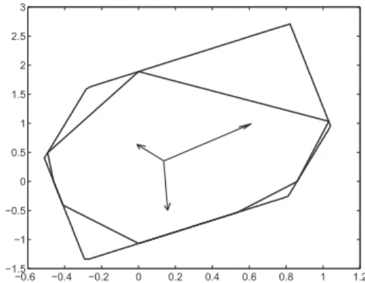
The Figure 3 (a) illustrates an example of the setV(~x,dˇ)obtained initially with the vectors
v1=[1;1.1]; v2=[-0.2;0.6]; v3=[-0.21;-1.1];
In this Figure 3 (a), the external polygon was generated using as minimum and maximum values the vectors
Xmin=[-1,-1,-1]; Xmax=[1,1,1];
When we change the vector of minimum values of the control variables to
Xmin=[-0.1,-0.1,-0.1];
we obtain a new setV(~x,dˇ), which corresponds to the internal polygon. Notice how the polygon that representsV(~x,dˇ)loses its symmetry about the origin whenXminis different from-Xmax. We remark that the number of directions used to determine the region can influence the quality of the set of possible velocities generated. The Figure 3 (b) illustrates a setV(~x,dˇ)given by the values
v1=[1;1.1]; v2=[-0.2;1.6]; v3=[-0.21;-1.1];
where the internal polygon was generated using 8 directions and the external polygon was generated using 320 directions.
−1.5 −1 −0.5 0 0.5 1 1.5
−3 −2 −1 0 1 2 3
(a) With two different choices of minimum values of the control variables (see text).
−0.6 −0.4 −0.2 0 0.2 0.4 0.6 0.8 1 1.2
−1.5 −1 −0.5 0 0.5 1 1.5 2 2.5 3
With two different choices of the number of directions considered: 8 and 320.
Figure 3: Polygons representing the setV(~x,dˇ).
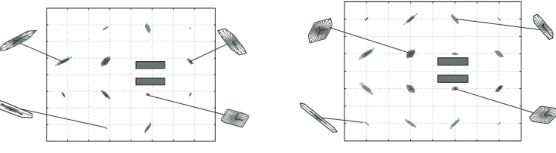
are of the pressure type, and in the Figure 4 (b) the actuators are of the electrode type. We can see the variability ofV(~x,dˇ), which is highly anisotropic and highly dependent on the geometric configuration as well as on the nature of the actuators. The regions where the polygons are smaller correspond to stagnant regions, i.e., regions where the velocity generated by the actuators hardly moves the particles at all. The regions where the polygons are bigger correspond to regions where the particles are easily transported. A “good” trajectory for manipulation avoids not just the obstacles but also these stagnant regions as much as possible.
(a) Actuators of the pressure type. (b) Actuators of the electrod type.
Figure 4: Representation of the setV(~x,dˇ)of the possible maximum velocities (in each of the 32 directions considered) in some points of the domain.
4 OPTIMIZING TRAJECTORIES BY BELLMAN’S PRINCIPLE
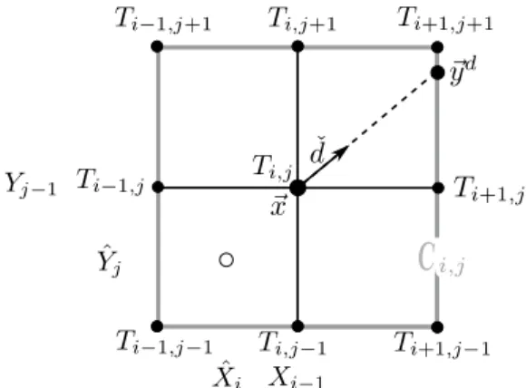
The optimal trajectory, in terms of time, for moving a particle from a point~xto a target point, solves the Hamilton-Jacobi-Bellman equation. A semi-Lagrangian discretization is considered for the functionT . The equation (2.6) is approximated at each node(i,j), taking the curveC
(denoted asCi,j) as the boundary of the set of the four cells that share node(i,j). The coordinates of node(i,j)are~x= (Xi−1,Yj−1)(see Figure 5). For each direction ˇd, the trajectory from~xto
Ci,jis approached by a straight line from~xto~yd∈Ci,j.
The values for the discrete approximation ofTi,jare defined by
Ti,j= min kdˇk=1
T(~yd) +k~x−~y dk
V(~x,dˇ)
whereT(~yd)is an interpolation of theT values at the nodes that are placed onCi,j. In the case of the direction ˇdillustrated in the Figure 5, for example,T(~yd)is calculated by linearly interpolat-ing betweenTi+1,jeTi+1,j+1. The direction of the optimal trajectory is that in which the minimum
is attained, which is generally not parallel to∇T because of the anisotropy of the problem.
To leave a completely discrete scheme we consider the following discretization of the set of directionsD
D={dˇk= (cos(θk),sin(θk)),θ=
(k−1)π
C
Figure 5: Trajectory, approximated by a straight line, from~xtoCi,jfor the direction ˇd.
The algorithm requires thatV(~x,dˇ)has already been calculated at each vertex and has been stored as a table of valuesVik,j:=V(~xi,j,dˇk), corresponding to each vertex(i,j)and to each direction
ˇ
dk.Ti,jis initialized to a large value (1012) on all nodes except those that belong to the targetZ, which are initialized to zero. Then we iterate all the mesh nodes that do not belong toZupdating
T according with the following equation
Ti,j←− min ˇ d=dˇk∈D
(
T(~yd) +k~x−~y dk
Vik,j
)
. (4.1)
This algorithm is discussed in [5], including error estimators for the solution in the norm of
L∞(Ω), which is important because the exact solution in general is not smooth and can not be understood in the classical sense.
Remark 4.1(Complexity). Calculations necessary to start the previous algorithm are:
• Computing the matrixBaccording to the linear relation (2.1) for theNnodes andn actu-ators with costnO(Na), whereO(Na)is the cost of solving one hydrodynamic problem (tipicallya≈ from 1.3 to 1.5);
• Computing{Vi jk} with costmNO(nb), obtained by the costO(nb)of solving one linear optimization problem (2.3) in dimension n (tipicallyb≈2), for allN nodes and allm
directions.
From (4.1) the cost of the HJB iteration isO(mN), and the number of required iterations is O(N1/s), s being the number of space dimensions. Summarizing, the total cost adds up to
5 RESULTS
In this section, we consider the setDgenerated by 8 directions. The accuracy of the calculation depends on the number of the considered directions, and so does the computational cost. The choice of 8 directions has the advantage of not requiring the interpolation step, since the direc-tions considered in (4.1), withk=1, . . . ,8, are determined by the neighboring nodes. Therefore for each node(i,j)the optimal trajectory is a line that connects it to the neighboring mesh node at which the minimum in (4.1) is attained. As a consequence, the set of numerical trajectories produced by our algorithm has a tree structure. For this reason, to plot the numerical solution we draw all the optimal trajectories that pass through the mesh nodes, which has the geometrical appearance of a tree rooted at the targetZ.
In the next simulations, we consider a domainΩ={(x1,x2)∈R2,0<x1,x2<10}discretized in a
grid of 40×40 nodes, except when indicated otherwise. When the flux is induced by an electrical potential we assume an electrosmotic costantmeo=1 while when it is generated by a pressure source we consider viscosityµ=0.1. The actuators’ limit values are set toX−= (−1,−1,−1) andX+= (1,1,1).
Figure 6 shows the trees of optimal trajectories obtained for both electrical (subfigure (a)) and mechanical (subfigure (b)) actuators.
(a) Electrical potential. (b) Pressure.
Figure 6: Optimal trajectory configuration with range of actuators between −1 and 1. The destacked point is the arrival target.
the obstacle so as to traverse regions (more distant to the obstacle) where the admissible veloci-ties are higher. Notice also that the trajectory trees have similariveloci-ties for both types of actuators, mainly differing at the obstacles’ boundaries, where the mechanically-driven flow has zero ve-locity while the electrically-driven one only imposes the normal component of the veve-locity to be zero.
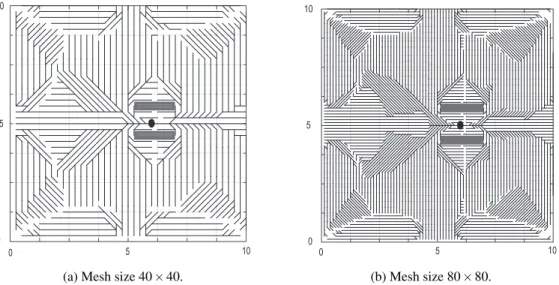
The model exhibits convergent behavior with respect to mesh refinement in all cases considered. As an example, in Figure 7 we compare the resulting trees for the electrically-driven model, with meshes 40×40 and 80×80.
(a) Mesh size 40×40. (b) Mesh size 80×80.
Figure 7: Effect of mesh refinement on the resulting trajectory trees, for the electrically-driven flow.
The optimal trajectories may be counterintuitive. Let us consider the flow generated by pressure actuators setting as target Z a single point close to the obstacle as shown in Figure 8. Then we consider two possible start points, labeled with the lettersAandB. In the case with Aas starting point, the model designs an optimal trajectory that is a straight segment. The travel time
tcomputed by integrating the fieldV(·,dˇ)betweenAandZalong a straight line ( ˇτ1=1, ˇτ2=0)
fundamental result since it avoids obstacles and stagnant regions. This path can then be traveled at non-optimal velocities, with smoother control functions, as discussed in Remark 2.1.
0 0
Arrival point Optimal trajectory Straight trajectory t = 9.1
op t = 6.7
t = 4.4
op t = .4 4 A
B
10 5
10
5
Figure 8: Comparison of the optimal trajectories with straight ones.
Time
0 1 2 3 4 5 6 7
Pre
ssu
re
-1 -0.5 0 0.5 1
X X X N
W
S
Figure 9: Actuators values over time along the optimal path starting atB.
6 CONCLUSIONS
We have presented an integrated model to identify convenient trajectories for the manipulation and control of particles in microfluidics. The achievement of the above-mentioned objective involved various mathematical problems:
– a Stokes problem for the velocity field induced by pressure sources;
– a Poisson problem for the electrical potential induced by a voltage imposed at electrodes, which in turn induces an electrosmotic velocity field;
• To determine the maximum admissible velocity V(~x,dˇ) at each point~x and for each direction ˇd, through the resolution of a linear optimization problem;
• To provide the control functions X∗(t) arising from the resolution of an initial value problem for the trajectory ODE;
• To plan the trajectory by minimizing the arrival time through the numerical implementation of Bellman’s principle.
The proposed method automatically indentifies a trajectory for a particle that we must manipulate from a departure point to the target in minimum time (and also provides the corresponding values to impose on the actuators). The numerical results show that the trajectories found not only avoid the obstacles, but also avoid the regions of the domain where the actuators are ineffective at producing flow. The numerical simulations show counterintuitive optimal trajectories in this kind of problem, justifying the use of mathematical models for designing automatic manipulation systems.
It should be noted that the proposed algorithm produces not just one optimal trajectory, but the whole tree of optimal paths, starting at anyx∈Ω. This apparent overkill is very important when applying the model under realistic conditions, in particular considering external perturbations (noise). In fact, if the sensor in the control loop detects that a perturbation has taken the particle to a position ˜xoutside the original optimal path, the controller can immediately switch to the path in the optimal tree that passes throught ˜x. In this way, and without any additional computation, the optimal tree can be used to correct perturbations so that the particle eventually reachesZ.
ACKNOWLEDGEMENTS
This work was carried out with the financial support of the CAPES and CNPq agencies. In partic-ular, Luca Meacci acknowledges for the financial support the Programa de Excelˆencia Acadˆemica (Proex) – Coordenac¸˜ao de Aperfeic¸oamento de Pessoal de N´ıvel Superior – Brazil (CAPES) – Finance Code PROEX-9740044/D.
pixeladas. Simulac¸˜oes num´ericas mostram que a ´arvore de trajet´orias obtida do algoritmo evita obst´aculos e regi˜oes estagnadas do dom´ınio flu´ıdico com sucesso.
Palavras-chave: Planejamento de trajet´oria, manipulac¸˜ao de part´ıculas em microflu´ıdica, Princ´ıpio de Bellman.
REFERENCES
[1] M. Armani, S. Chaudhary, R. Probst, S. Walker & B. Shapiro. Control of microfluidic systems: two examples, results, and challenges.International Journal of Robust and Nonlinear Control,15(16) (2005), 785–803.
[2] M. Armani, Z. Cummins, J. Gong, P. Mathai, R. Probst, C. Ropp, E. Waks, S. Walker & B. Shapiro. Feedback Control of Microflows. In “Feedback Control of MEMS to Atoms”. Springer (2012), pp. 269–319.
[3] S. Cacace, E. Cristiani & M. Falcone. Can Local Single-Pass Methods Solve Any Station-ary Hamilton–Jacobi–Bellman Equation? SIAM Journal on Scientific Computing, 36(2) (2014), A570–A587.
[4] S. Chaudhary & B. Shapiro. Arbitrary steering of multiple particles independently in an electro-osmotically driven microfluidic system.IEEE Transactions on Control Systems Technology,14(4) (2006), 669–680.
[5] E. Cristiani. “Numerical methods for optimal control problems: part II: local single-pass methods for stationary HJ equations”. IAC-CNR, Roma (2013). p. 21. Class notes.
[6] J.E. Curtis, B.A. Koss & D.G. Grier. Dynamic holographic optical tweezers.Optics communications, 207(1) (2002), 169–175.
[7] B.J. Kirby. “Micro-and nanoscale fluid mechanics: transport in microfluidic devices”. Cambridge university press (2010).
[8] P.P. Mathai, A.J. Berglund, J.A. Liddle & B.A. Shapiro. Simultaneous positioning and orientation of a single nano-object by flow control: theory and simulations.New Journal of Physics,13(1) (2011), 013027.
[9] L. Meacci, F.F. Rocha, A.A. Silva, P.V. Pramiu & C.G. Buscaglia. Planejamento de trajet´oria para a manipulac¸˜ao de part´ıculas em microflu´ıdica.CQD-Revista Eletrˆonica Paulista de Matem´atica,10 (2017), 19–37.
[10] R. Probst & B. Shapiro. Three-dimensional electrokinetic tweezing: device design, modeling, and control algorithms.Journal of Micromechanics and Microengineering,21(2) (2011), 027004.
[11] J.A. Sethian & A. Vladimirsky. Ordered upwind methods for static Hamilton–Jacobi equations.
Proceedings of the National Academy of Sciences,98(20) (2001), 11069–11074.
[12] I. Tuval, I. Mezi´c, F. Bottausci, Y.T. Zhang, N.C. MacDonald & O. Piro. Control of particles in microelectrode devices.Physical review letters,95(23) (2005), 1–4.