3D numerical modelling of subduction initiation at a passive margin

UNIVERSIDADE DE LISBOA

FACULDADE DE CIÊNCIAS

DEPARTAMENTO DE ENGENHARIA GEOGRÁFICA, GEOFÍSICA E ENERGIA

3D NUMERICAL MODELLING OF SUBDUCTION

INITIATION AT A PASSIVE MARGIN

Frederico Manuel Raposo Cabral

Mestrado em Ciências Geofísicas

(Geofísica Interna)

UNIVERSIDADE DE LISBOA

FACULDADE DE CIÊNCIAS

DEPARTAMENTO DE ENGENHARIA GEOGRÁFICA, GEOFÍSICA E ENERGIA

3D NUMERICAL MODELLING OF SUBDUCTION

INITIATION AT A PASSIVE MARGIN

Frederico Manuel Raposo Cabral

Mestrado em Ciências Geofísicas

(Geofísica Interna)

Tese orientada pelo Professor Doutor Fernando Manuel Ornelas Guerreiro Marques

II

Resumo

A subducção é um processo chave na teoria da tectónica de placas. Todavia, apesar de todos

os esforços realizados nas últimas décadas no estudo deste processo, o início da subducção

ainda não é totalmente compreendido. Actualmente, não existem claras evidências da

passagem de margens passivas para margens activas, muito embora as margens passivas

representem os locais mais prováveis para a ocorrência de subducção. É actualmente aceite

que a litosfera oceânica apresenta um valor negativo de impulsão que favorece o início da

subducção, contudo o balanço entre as forças de atrito e elásticas (como forças resistivas) e as

forças de abertura oceânica e gravitacionais (como forçadoras) previne o início de subducção.

Desta forma, outros parâmetros devem ser tidos em conta para explicar o início da subducção,

tais como a espessura da crosta continental e da litosfera continental e ainda os contrastes

laterais de densidade entre as litosferas oceânica e continental. Os estudos mais recentes

tentam perceber o problema através de modelos analíticos, analógicos e numéricos, todavia,

todos os estudos consideram as zonas de subducção como um problema 2D, embora estas

zonas tenham formas 3D na natureza. Tendo em conta as formas mais complexas das margens

passivas tentamos neste trabalho, através de modelação numérica 3D, investigar os efeitos de

diferentes geometrias da fronteira entre o oceano e o continente no início da subducção e

testar se existem assim geometrias mais favoráveis ao início da subducção.

Os resultados dos nossos testes indicam que a geometria sem variação entre as placas

litosféricas é mais provável para o início da subducção, visto que nos testes com geometrias

da fronteira oceano-continente a variar na terceira dimensão aumentarem o tempo para a

ocorrência de subducção ou até impossibilitarem o início de subducção.

III

Abstract

Subduction is one of the key processes in the plate tectonics theory. However, despite

all efforts in the last decades studying this problem, subduction initiation at passive margins is

not yet fully understood. Present-day transition from passive to active margin is not obvious,

although passive margins look like the most probable places for subduction initiation to occur.

Despite the favourable negative buoyancy of oceanic lithosphere, the force balance between

elastic and frictional forces (as resisting forces) and ridge push and gravitational forces (as

driving forces) seems to inhibit the initiation of subduction. Therefore, other parameters must

be taken into account in subduction initiation, like thickness of continental crust and

lithosphere, and lateral density contrasts between continental and oceanic lithospheres. The

recent studies that tried to solve this enigma vary from analytical, analogue and numerical

approaches; however all of them treat the subduction zone as a 2D problem, despite these

zones have a 3D shape. Given the complex shape of most passive margins, we use numerical

modelling in 3D to investigate the effects of different geometries of continental-oceanic

boundaries on subduction initiation, and to test if one of these geometries is more prone to

initiate subduction.

Our results show that the most prone geometry to initiate subduction at a passive

margin is the usual third dimension invariant, common of the 2D models (without any angle

in the the oceanic-continental boundary respecting to third dimension). More, our results

indicate that with the increasing angle in the oceanic-continental lithospheres (e.g. 20, 40 or

60 degrees) the subduction tend to be retard, and for the highest angels the subduction can be

even prevented.

Key Words:

V

Contents

Resumo ... II Palavras Chave: ... II Abstract ... III Key Words: ... III List of Figures ... VII List of Tables ... X 1. Introduction ... 1 1.1 The problem ... 1 1.2 Methodology ... 1 1.3 Outline ... 1 1.4 Theoretical Introduction ... 1 2. Model Description ... 5

2.1 Initial and Boundary Conditions ... 5

3. Results and discussion ... 12

3.1 Reference Model ... 12 3.2 Experiments f1 ... 14 3.2.1 Experiment f1a_f0i ... 14 3.2.2 Experiment f1b_f0i ... 16 3.2.3 Experiment f1c_f0i ... 19 3.3 Experiments f2 ... 22 3.3.1 Experiment f2a_f0i ... 22 3.3.2 Experiment f2b_f0i ... 24 3.3.3 Experiment f2c_f0i ... 26 4. Conclusion ... 30 5. Bibliography ... 30

VII

List of Figures

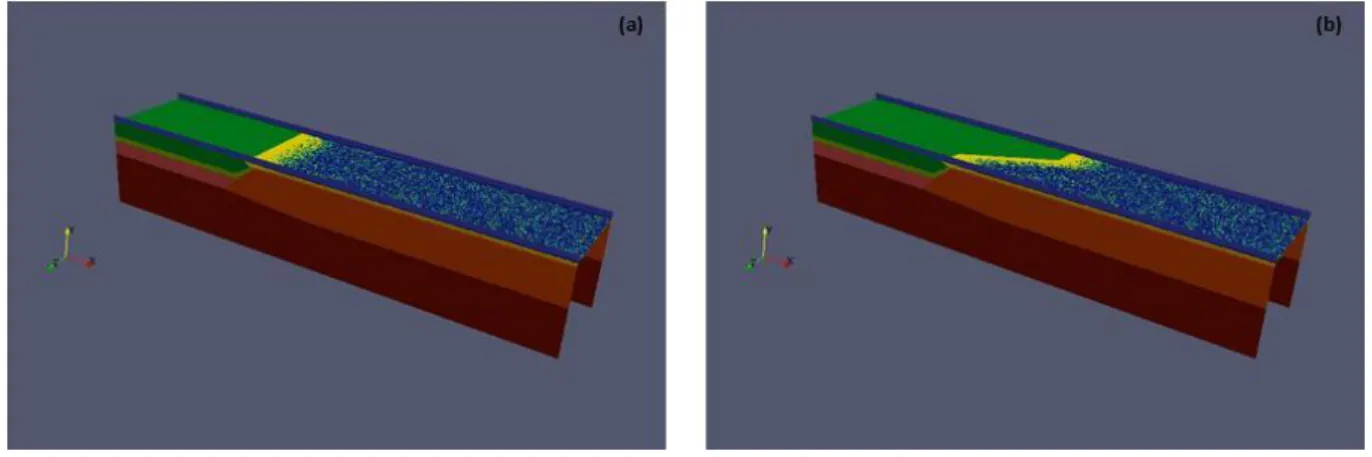
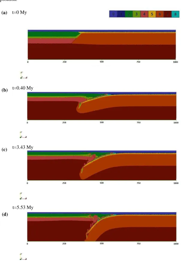
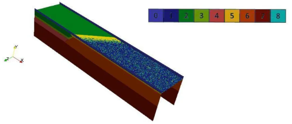
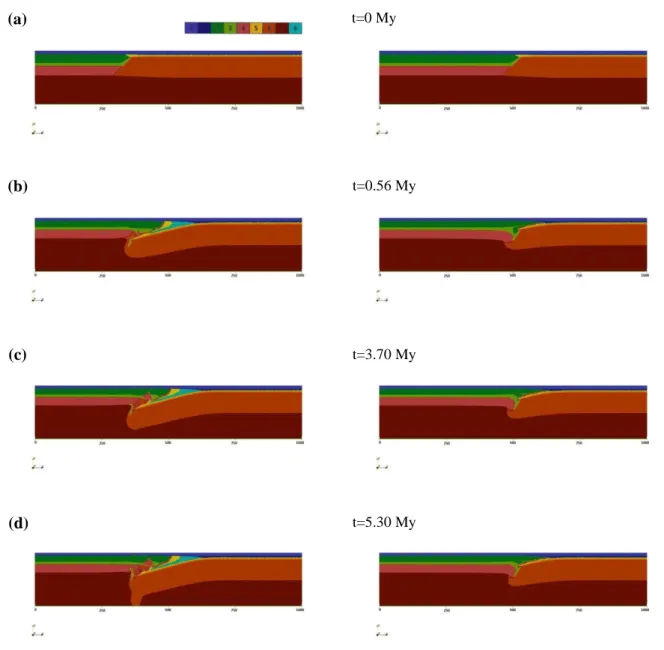
Fig. 1- 3D scheme of an oceanic-continental boundary (a) invariant in the third dimension (equivalent to 2D), and (b) variant in the third dimension (3D). ... 5 Fig. 2 - The (a) composition, (b) temperature and (c) viscosity fields of the initial configuration of the reference model. Colours for the composition field are numbered as follows: 0, air; 1, water; 2, upper continental crust; 3, lower continental crust; 4, continental mantle; 5, oceanic crust; 6, oceanic mantle; 7, asthenosphere. ... 7 Fig. 3 - (a) Boundary names and conditions; (b) Scheme of the f1 experiments (e.g. θ=60° ); (c) Scheme of the f2 experiments (e.g. θ=60). In (c) the thickness of the straight sections is 50 km each and the oblique section has 100 km (z maximum 200 km). Colours for the composition field are numbered as in Fig.2 with the addition of sediments (number 8). ... 10 Fig. 4 - Initial composition profiles from the reference model. Colours for the composition field are numbered as in Fig.2 with the addition of sediments (number 8). ... 12 Fig. 5 - Temporal evolution of the composition field from the reference model. Time steps: (a) 0 My; (b) 0.38 My; (c) 3.38 My (self sustained subduction); (d) 7.28 My. The horizontal scale represents the distance in kilometres from the left boundary. Colours for the composition field are numbered as in Fig.2 with the addition of sediments (number 8). ... 13 Fig. 6 - Initial composition profiles from the f1a_f0i experiment (θ=20). Colours for the composition field are numbered as in Fig.2 with the addition of sediments (number 8). ... 14 Fig. 7 - Temporal evolution of the composition field from the f1a_f0i experiment in the front boundary (left side) and back boundary (right side). Time steps: (a) 0 My; (b) 0.40 My; (c) 3.43 My (self sustained subduction in the front boundary); (d) 5.53 My; (e) 10.48 My. The horizontal scale represents the distance in kilometres from the left boundary. Colours for the composition field are numbered as in Fig.2 with the addition of sediments (number 8). ... 15 Fig. 8 - Initial composition profiles from the f1b_f0i experiment (θ=40). Colours for the composition field are numbered as in Fig.2 with the addition of sediments (number 8). ... 16 Fig. 9 - Temporal evolution of the composition field from the f1b_f0i experiment in the front boundary (left side) and back boundary (right side). Time steps: (a) 0 My; (b) 0.56 My; (c) 3.70 My; (d) 5.30 My. The horizontal scale represents the distance in kilometres from the left boundary. Colours for the composition field are numbered as in Fig.2 with the addition of sediments (number 8). ... 17

VIII Fig. 10 - Temporal evolution of the temperature field from the f1b_f0i experiment in the front boundary. Time steps: (a) 0 My; (b) 0.56 My; (c) 3.70 My; (d) 5.30 My. The horizontal scale represents the distance in kilometres from the left boundary. Colours for the composition field are numbered as in Fig.2 with the addition of sediments (number 8). ... 18 Fig. 11 - Initial composition profiles from the f1c_f0i experiment (θ=60). Colours for the composition field are numbered as in Fig.2 with the addition of sediments (number 8). ... 19 Fig. 12 - Temporal evolution of the composition field from the f1c_f0i experiment in the front boundary (left side) and back boundary (right side). Time steps: (a) 0 My; (b) 0.27 My; (c) 3.75 My; (d) 6.15 My. The horizontal scale represents the distance in kilometres from the left boundary. Colours for the composition field are numbered as in Fig.2 with the addition of sediments (number 8). ... 20 Fig. 13 - Temporal evolution of the temperature field from the f1c_f0i experiment in the front boundary. Time steps: (a) 0 My; (b) 0.27 My; (c) 3.75 My; (d) 6.15 My. The horizontal scale represents the distance in kilometres from the left boundary. Colours for the composition field are numbered as in Fig.2 with the addition of sediments (number 8). ... 21 Fig. 14 - Initial composition profiles from the f2a_f0i experiment (θ=20). Colours for the composition field are numbered as in Fig.2 with the addition of sediments (number 8). ... 22 Fig. 15 - Temporal evolution of the composition field from the f2a_f0i experiment in the front boundary (left side) and back boundary (right side). Time steps: (a) 0 My; (b) 0.39 My; (c) 4.63 My; (d) 6.14 My. The horizontal scale represents the distance in kilometres from the left boundary. Colours for the composition field are numbered as in Fig.2 with the addition of sediments (number 8). ... 23 Fig. 16 - Evolution of the temperature field from the f2a_f0i experiment in the front boundary (left side) and back boundary (right side) at (a) 0.39 My and (b) 6.14 My. The horizontal scale represents the distance in kilometres from the left boundary. ... 24 Fig. 17 - Initial composition profiles from the f2b_f0i experiment (θ=40). Colours for the composition field are numbered as in Fig.2 with the addition of sediments (number 8). ... 24 Fig. 18 - Temporal evolution of the composition field from the f2b_f0i experiment in the front boundary (left side) and back boundary (right side). Time steps: (a) 0 My; (b) 0.41 My; (c) 4.72 My; (d) 7.11 My; (e) 9.47 My. The horizontal scale represents the distance in kilometres from the left boundary. Colours for the composition field are numbered as in Fig.2 with the addition of sediments (number 8). ... 25 Fig. 19- Temperature profiles from the f2b_f0i experiment in the front boundary (left side) and back boundary (right side) at 9.47 My. The horizontal scale represents the distance in kilometres from the left boundary. ... 26

IX Fig. 20 - Initial composition profiles from the f2c_f0i experiment (θ=60). Colours for the composition field are numbered as in Fig.2 with the addition of sediments (number 8). ... 27 Fig. 21- Temporal evolution of the composition field from the f2c_f0i experiment in the front boundary (left side) and back boundary (right side). Time steps: (a) 0 My; (b) 0.50 My; (c) 4.43 My; (d) 7.62 My. The horizontal scale represents the distance in kilometres from the left boundary. Colours for the composition field are numbered as in Fig.2 with the addition of sediments (number 8). ... 28

X

List of Tables

Table 1 - Parameters used in the numerical experiments. ... 8 Table 2 - List of experiments. The suffix “_f0g” and “_f0i” respects to the reference model. The suffix “a”,”b” or “c” after the experiment type 1 and 2 (e.g. f1a) respects to the θ angle, where a=20°, b=40°, c=60°. ... 11 Table 3 - Summary of experiment results. ... 29

3D NUMERICAL MODELLING OF SUBDUCTION INITIATION AT A PASSIVE MARGIN

Frederico Cabral 1

1. Introduction

1.1 The problem

Subduction zones are one of the most important features in the plate tectonic theory. In the last decades many studies have been done to understand the dynamics involved in the subduction initiation, and these approaches used analytical, analogue and numerical models trying to understand all the forces and dynamics involved in the subduction initiation. However, most of the conclusions resulting from these works are simply in a 2D view. Although is known that subduction is a 3D problem and this way we try to investigate, using numerical modelling, the best geometry of the continental and oceanic plates in the third dimension that promote the subduction initiation.

1.2 Methodology

A 3D approach to subduction zones is very complex because of the large number of features necessary to study this subject. This way to best understand the subduction initiation we used numerical modelling that can give us a new knowledge on this process. The numerical approach were performed using the I3ELVIS code, that is based on finite differences schemes and based-in-cell techniques combined with multigrid approach, a additional feature to the previous I2ELVIS code in 2-D (Gerya and Yuen, 2007). The models include a free surface as well as phase transformation and water transport.

1.3 Outline

The current work is divided in four main parts. In the first chapter, the Introduction, contents the basics to understand the subject and gives an overview of the past work done in this field. In the second chapter we present our model and the initial and boundary conditions. In the third section are present and discuss the first results of the numerical simulation that confirms the similarities of our model with previous studies, and the results from simulations testing different geometries between the oceanic-continental boundary. The chapter four we discuss our results and in the chapter five, last chapter our main conclusions.

1.4 Theoretical Introduction

Since the beginning of the plate tectonics theory, different types of studies have been carried out trying to understand the dynamics involved in the process of subduction initiation; however, many aspects are still not entirely understood.

It is reasonably well established that due to oceanic lithosphere aging and cooling its density increases (Oxburgh and Parmentier 1977); therefore, an instability arises and the plate should, in principle, sink spontaneously into the mantle under its own weight (Turcotte et al. 1977).

3D NUMERICAL MODELLING OF SUBDUCTION INITIATION AT A PASSIVE MARGIN

Frederico Cabral 2

However, Mckenzie (1977) calculated the force balance present at passive margins assuming an elastic rheology and concluded that spontaneous subduction is not possible under common gravitational forces. In his calculations he considered the balance between the elastic resistance (due to bending resistance of the oceanic lithosphere) and frictional resistance (friction at the thrust contact between underthrusting and overriding plates), as resistance forces, and ridge-push and gravitational instability as driving forces. He calculated the balance between these forces to initiate subduction at a passive margin, and concluded that an additional stress of 80MPa, resulting from the force integration over common elastic thickness of the lithosphere (80km), is required for subduction initiation and subsequent self sustained subduction driven by slab-pull. Moreover, in order for slab-pull to act in efficiently, the density contrast between the sinking slab and the surrounding mantle must be preserved; therefore, if the consumption rate is not high enough (> 1.8cm/yr) the density contrast can be reduced due to warming of the sinking slab thus preventing subduction initiation.

Different studies were performed after Mckenzie (1977), trying to find a mechanism that enables subduction initiation. The possibility of a fracture zone, representing a weakness in the oceanic-continental boundary, was one of the most reasonable approaches to solve the problem of extra forces, because frictional resistance should be reduced with a fracture zone.

Cloetingh (1982) estimated the stress produced by a sedimentary load at a passive margin with ductile lithosphere. However, he concluded that a plastic failure due to sedimentary load is just possible in oceanic lithosphere younger than 20 My. This way the stress resulting from sedimentary load is not able to reach the strength of the lithosphere due to its increase with increasing age and cooling.

Another study to explain subduction initiation was performed by Mueller and Phillips (1991) through analytical models, which tried to estimate the shear resistance forces at passive margins, fracture zones, transform faults and extinct ridge assuming a brittle-ductile rheology. The study concluded that, for passive margins, the magnitude of the shear resistance forces are one order of magnitude higher than ridge-push. Although they suggest that subduction can be initiated due to the slab pull forces from other mature subduction zones in the proximities, this does not explain the initiation of the first subduction zone.

Regenauer-Lieb et al. (2001) estimated that the addition of water changes the rheology of the upper and middle lithosphere and the shear resistance forces can be reduced leading to the development of an instability explaining the subduction initiation; however their estimations were applied to oceanic lithosphere instead of passive margins.

Toth and Gurnis (1998) used numerical modelling to estimate new values for the resistance forces in the case of a preexisting fault and even found a relation for the necessary driving force that exceed the resistance forces needed to initiate subduction. Despite the efforts to explain initiation of subduction by the presence of a fracture zone, many of these studies do not take into account other

3D NUMERICAL MODELLING OF SUBDUCTION INITIATION AT A PASSIVE MARGIN

Frederico Cabral 3

parameters that can explain the process in passive margins, a likely place for subduction initiation to occur.

Another approach to the problem was made by Faccena et al. (1999), using analogue models where they investigate the influence of the negative buoyancy of the oceanic lithosphere, the horizontal body forces between continent and ocean that result from lateral density contrasts, and brittle and ductile strengths of the passive margin. Using the Argand number (representing the ratio between body force of continent and its integrated strength) and the buoyancy number (representing the ratio between the buoyancy force of the ocean and its ductile resistance) they predicted that with a higher body force together with a high buoyancy force on the oceanic plate presents the best similarities with passive margins like the Atlantic-type.

From the development made by Faccena et al. (1999), a new set of gravitational forces must be taken into account to explain subduction initiation. Mart et al. (2005) performed an analogue study just considering gravitational forces, without any lateral compression, and the results show thrusting of the continental lithosphere over the higher density oceanic slab, mainly controlled by the degree of friction and density contrast between the two plates.

Goren et al. (2008), trying to understand more about the influence of the gravitational forces, reported that the effects of lateral buoyancy differences can trigger a lateral pressure gradient from the oceanic to the continental lithospheres. The study performed by Goren et al. (2008), trough analytical and analogue models, predicted that these lateral forces reach the maximum value at the base of the lithosphere and can induce viscous deformation at the ductile portion of the lithosphere. This way, in the beginning the oceanic-continental boundary stays under a compression regime leading to elevation differences responsible for topographic features in the continental lithosphere. In response to this new unstable isostatic configuration, the continental lithosphere can initially overthrust the oceanic lithosphere, due to isostatic rearrangement, and a low angle subduction can occur. Development after this initial state can occur with the sinking of the oceanic slab, due to gravitational instability between the denser oceanic lithosphere and the lighter asthenospheric mantle. However their results do not show a proper subduction zone with a deep sinking oceanic slab into asthenospheric mantle, but rather showed different cases of overthrusting with the continental lithosphere creeping over the deflected oceanic lithosphere.

The lateral pressure gradient in passive margins emerges from lateral density contrasts. These lateral density differences result from compositional differences from continental and oceanic rocks, and these differences can be obtained by isostatic adjustments; however, temperature variations can lead to lithosphere density variations that may overlap the isostatic processes. In addition lateral density variations between lithospheric mantles can reinforce the lateral pressure gradient at passive margins, and these lateral differences are typically attributed to melting processes originated by

3D NUMERICAL MODELLING OF SUBDUCTION INITIATION AT A PASSIVE MARGIN

Frederico Cabral 4

temperature effects. Therefore, with numerical modelling, the effects of temperature can be taken into account.

Nikolaeva et al. (2010) performed a serious of 2D numerical experiments with viscoelastoplastic rheology and investigated the effects of lithospheric thickness, chemical density contrast between the continental and oceanic lithospheric mantles, age of oceanic plate, and plastic strength and thickness of the continental crust. In this work they achieve three distinguish regimes at a passive margin: stable margin, overthrusting, and subduction. Thus they concluded that the transition from stable margin to overthrusting is mainly controlled by ductile strength of the continental crust. The transition from overthrust to subduction initiation is mainly controlled by ductile strength and density of the continental lithosphere. Another conclusion from their work was the small contribution of the age of the oceanic plate, which controls the thickness and strength of this plate, and a similar conclusion arise from the study of Goren et al. (2008) in their experiments with a buoyancy number equal to zero.

The 2-D numerical approaches have provided improvements in the knowledge of the dynamics of subduction initiation, but they only apply to situations where the third dimension is invariable (Fig.1 (a)). However, the real world is not so simple, and shows variations (at least geometric) of the third dimension (Fig.1 (b)). In fact, the natural passive margins are not straight, and even less perpendicular to the velocity vector. Therefore, in order to fully understand subduction initiation, the three spatial coordinates of the stress tensor must be considered.

In our study we follow the previous works, but because of the 3D shape of the real subduction zones and the 3D spatial distribution of stress we used a 3D numerical model with viscoelastoplastic rheology to perform different experiments to investigate the influence of different geometries of the ocean-continental boundary in the third dimension on subduction initiation at a passive margin. In our model we take into account as driving forces only the lateral density variations between the oceanic-continental boundary. We did not consider any type of differences in the rock composition of the same plate along the third dimension. This way we ensure pressure gradients related to density contrast only between the oceanic and continental lithospheres.

3D NUMERICAL MODELLING OF SUBDUCTION INITIATION AT A PASSIVE MARGIN

Frederico Cabral 5

Fig. 1- 3D scheme of an oceanic-continental boundary (a) invariant in the third dimension (equivalent to 2D), and (b) variant in the third dimension (3D).

2. Model Description

The numerical code used in this work is the I3ELVIS code, which is based on finite differences schemes and marker-in-cell techniques combined with multigrid approach, an additional feature to the previous I2ELVIS code in 2D (Gerya and Yuen 2007).

The model can be seen as a mixed Lagrangian-Eulerian numerical scheme and is applicable to Cartesian geometry with prescribed vertical gravity field allowing to model regional tectonic processes in 3D, with viscoelastoplastic rheology.

The model accounts for the dynamics of free surface, spontaneous slab bending, back-arc spreading and thermal-chemical plumes propagation; however, this last routine was not performed in order to reduce the computational time spent running the experiments.

To ensure a realistic one sided (Gerya et al. 2008) subduction pattern, the model accounts for slab dehydration processes on the basis of the Gibbs free energy minimization combined with the moving fluid markers technique (Gerya et al. 2006; Nikolaeva et al. 2008).

2.1 Initial and Boundary Conditions

The present 3D model is a reference model of subduction initiation at passive margins. The model domain is 1000 km long orthogonal to the oceanic-continental boundary, 200 km deep and 200 km wide. This domain is resolved by 501x101x101 grid points with approximately 43 million randomly distributed markers. The model has a prescribed gravity field oriented vertically with 9.8 ms -2

, and no velocities are imposed at the boundaries. In the experiments the composition of rocks follows a viscoelastoplastic rheology (e.g. Ranalli 1995). A total of 38 rock phases are defined in the model plus an air description to account for free surface conditions, however the most important composition

3D NUMERICAL MODELLING OF SUBDUCTION INITIATION AT A PASSIVE MARGIN

Frederico Cabral 6

of the model can be described using just nine layers (air, water, upper continental crust, lower continental crust, continental mantle, oceanic crust, oceanic mantle, asthenosphere and sediments).

We built a reference model (f0i Table 2) that simulates subduction initiation at an oceanic-continental boundary, invariable in the third dimension (Fig.2). Therefore, the results of this model were a reference to compare with all different experiments carried out in this work. However, in order to test only the geometry of the oceanic-continental boundary all the other parameters were kept unchanged.

The models are composed of a top 12 km layer of air that acts as a dynamically internal free surface, and represents the atmosphere (density 1 kgm-3 and viscosity 1018 Pas). Below, on the left side of the model, is the continental lithosphere, and on the right side the oceanic lithosphere (Fig.2 (a)).

The continental lithosphere is composed of upper and lower crust, above the continental mantle lithosphere. The continental upper crust has an average thickness of 33 km and is mainly composed of wet quartzite with a density of 2700 kgm-3 and a viscosity of 1026 Pas. The lower crust is 12 km thick and made of wet quartzite with a density of 2900 kgm-3 and a viscosity of 1018 Pas, responsible for the ductile behaviour. The continental mantle lithosphere is 35 km thick and is mainly composed of wet olivine with a viscosity of 1024 Pas and a density of 3250 kgm3 (50 kgm3 less than the neighbouring oceanic mantle lithosphere). Above the oceanic lithosphere there is a 3 km thick layer of water. The oceanic crust is mainly composed of 8 km thick basalts (An75) with an average density of 3100 kgm-3 and a viscosity of 1024 Pas. Below the oceanic crust is the oceanic mantle lithosphere with 77 km thickness of wet olivine with a density of 3300 kgm-3 and a viscosity of 1024 Pas. Beneath the two lithospheres is the asthenosphere to a total depth of 200km, and is mainly composed of wet olivine and has the same properties as the oceanic mantle lithosphere.

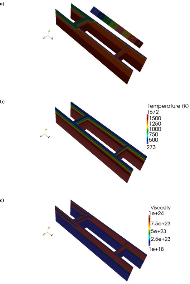
The most important properties of the different layers are presented in Table I. Note that the density contrast between the continental mantle lithosphere and the oceanic mantle lithosphere (50 kgm-3) is responsible for the gravitational instability at the margin and can drive subduction initiation (Nikolaeva et al. 2010). Furthermore, the viscosity of the lower continental crust is lower than the surrounding layers, and is thus responsible for the ductile behaviour of the continental lithosphere (Fig.2(c)).

The oceanic-continental boundary dips 45° towards the continent in almost all experiments (Fig.3 (b)); however, for the purpose of this work, in the third dimension (Z coordinate) the boundary changes between different angles (Fig.3 (b) and Table 2). The model oceanic crust does not include sediments, but they spontaneously fill the trench after its arcward slope reaches a critical angle of 17 degrees.

3D NUMERICAL MODELLING OF SUBDUCTION INITIATION AT A PASSIVE MARGIN

Frederico Cabral 7

Fig. 2 - The (a) composition, (b) temperature and (c) viscosity fields of the initial configuration of the reference model. Colours for the composition field are numbered as follows: 0, air; 1, water; 2, upper continental crust; 3, lower continental crust; 4, continental mantle; 5, oceanic crust; 6, oceanic mantle; 7, asthenosphere.

(a)

(b)

3D NUMERICAL MODELLING OF SUBDUCTION INITIATION AT A PASSIVE MARGIN

Frederico Cabral 8

The thermal structure in the model is composed of a linear profile in the continental lithosphere, which assumes 273 K at the surface and grows with depth by a temperature gradient of 0.5 Kkm-1. In the oceanic lithosphere the thermal profile is based on the imposed ages of the plate with an oceanic geotherm (Turcotte and Schubert 2002). The thermal structure in the oceanic-continental boundary is defined as an interpolation between the continental and oceanic profiles. The thermal conditions of our reference model can be seen in Fig.2 (b).

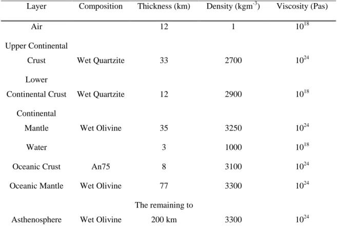
Table 1 - Parameters used in the numerical experiments.

Layer Composition Thickness (km) Density (kgm-3) Viscosity (Pas)

Air 12 1 1018

Upper Continental

Crust Wet Quartzite 33 2700 1024

Lower

Continental Crust Wet Quartzite 12 2900 1018 Continental

Mantle Wet Olivine 35 3250 1024

Water 3 1000 1018

Oceanic Crust An75 8 3100 1024

Oceanic Mantle Wet Olivine 77 3300 1024

Asthenosphere Wet Olivine

The remaining to

200 km 3300 1024

As mentioned above, the model has no applied boundary velocities, in order to test only the pressure gradient resulting from the density contrast at the oceanic-continental boundary. The velocity boundary conditions are free slip, except for the lower boundary, which is permeable in the vertical direction (Fig. 3 (a)). This boundary allows global conservation of mass in the computational domain.

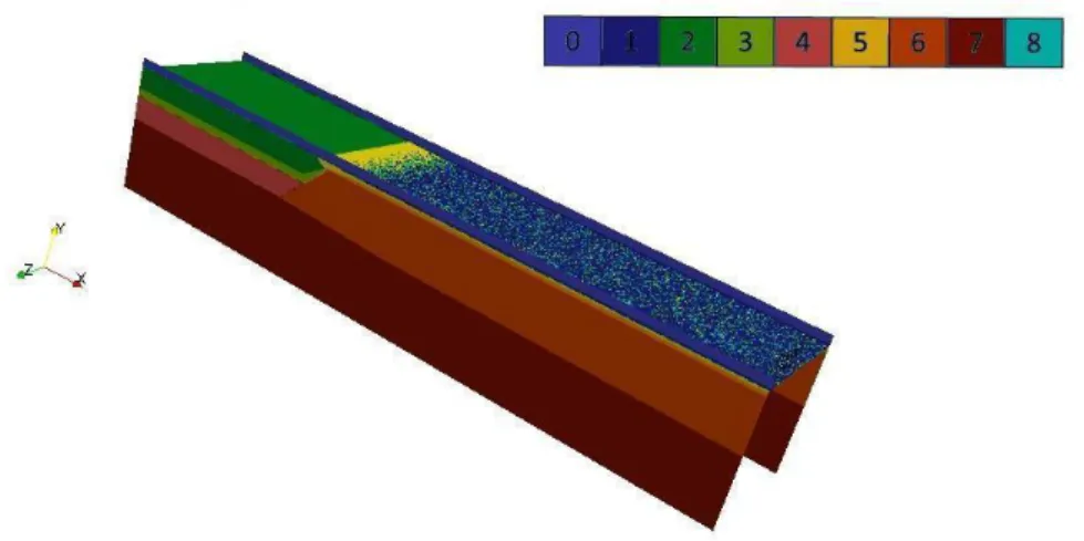
In order to help in the description of the results, it is important to distinguish some features of the computational domain and experiments. In the Fig. 3, the boundary names and their features are described, and two schemes are added to help to understand the different types of experiment. We defined three different types of experiment: the invariable in the third dimension, also defined as “f0” (Fig.3 (b) with θ = 0º); the oblique in the third dimension, defined as “f1” (Fig.3 (b)); the Z-shaped ocean-continent boundary, defined as “f2” (Fig.3 (c)). The difference between the three types of experiment is the geometry in the third dimension, while between the same types of experiment

3D NUMERICAL MODELLING OF SUBDUCTION INITIATION AT A PASSIVE MARGIN

Frederico Cabral 9

different features are tested. For experiments f0, our reference model, the variables are the thickness of the continental crust and the thickness of the continental mantle. In the f1 experiments the main variable was the angle θ, with the geometry of the oceanic-continental boundary following a linear profile along the third dimension (Fig.3 (b)). The f2 experiments are characterised by a Z-shaped profile, and we study the changes with the angle θ, as showed in Fig.3 (c), keeping the thickness (50 km each) of the invariant sections unchanged. Experiments f1 and f2 just show variations on the geometry of the oceanic-continental boundary in the third dimension and both keep all the other features of the reference model (f0i in Table 2).

In our work the angle α represents the slope in depth of continental lithospheres, and is assumed as 45 degrees and constant trough almost all experiments. The angle θ is the main variable in our study, and besides it may represent different displacement in different types of experiments. θ varied between 20, 40 or 60 degrees. The highlighted experiments in Table 2 are the ones presented in the Results section.

Notice that the compositional configuration in the front boundary remains the same in all experiments (the same values for the x coordinates), and this is important to relate different types of experiments and maintain coherency between then.

3D NUMERICAL MODELLING OF SUBDUCTION INITIATION AT A PASSIVE MARGIN

Frederico Cabral 10

Fig. 3 - (a) Boundary names and conditions; (b) Scheme of the f1 experiments (e.g. θ=60° ); (c) Scheme of the f2 experiments (e.g. θ=60). In (c) the thickness of the straight sections is 50 km each and the oblique section has 100 km (z maximum 200 km). Colours for the composition field are numbered as in Fig.2 with the addition of sediments (number 8).

(a)

(b)

3D NUMERICAL MODELLING OF SUBDUCTION INITIATION AT A PASSIVE MARGIN

Frederico Cabral 11

Table 2 - List of experiments. The suffix “_f0g” and “_f0i” respects to the reference model. The suffix “a”,”b” or “c” after the experiment type 1 and 2 (e.g. f1a) respects to the θ angle,

where a=20°, b=40°, c=60°. Experiments Density Contrast (kg/m3) Thickness Continental Crust (km) Thickness of Continental Mantle (km) Total Thickness Continental Lithosphere Total Depth Continental Lithosphere (km) Temperature at total depth of Continental Lithosphere (K) θ (°) α (°) Observations f0a 50 44 46 90 102 1624 0 45 f0b 50 44 46 90 102 1624 0 45 f0c 50 44 34 78 90 1618 0 45 f0d 50 44 44 88 100 1623 0 45 f0f 50 45 43 88 100 1623 0 45 f0g 50 45 30 75 87 1616.5 0 45 f0i 50 45 35 80 92 1619 0 45 f0ia 50 45 35 80 92 1619 0 45 Oceanic lithosphere with 430 km f0ib 50 45 35 80 92 1619 0 45 Oceanic lithosphere with 230 km f0j 50 43 30 73 85 1615.5 0 45 f1a_f0g 50 45 30 75 87 1616.5 20 45 f1a_f0i 50 45 35 80 92 1619 20 45 f1b_f0g 50 45 30 75 87 1616.5 40 45 f1b_f0i 50 45 35 80 92 1619 40 45 f1b 50 45 35 80 92 1619 40 0 f1c_f0g 50 45 30 75 87 1616.5 60 45 f1c_f0i 50 45 35 80 92 1619 60 45 f2a_f0g 50 45 30 75 87 1616.5 20 45 f2a_f0i 50 45 35 80 92 1619 20 45 f2b_f0g 50 45 30 75 87 1616.5 40 45 f2b_f0i 50 45 35 80 92 1619 40 45 f2c_f0g 50 45 30 75 87 1616.5 60 45 f2c_f0i 50 45 35 80 92 1619 60 45

3D NUMERICAL MODELLING OF SUBDUCTION INITIATION AT A PASSIVE MARGIN

Frederico Cabral 12

3. Results and discussion

In this section we present the results of our experiments for the reference model (f0i) and for tree other experiments from experiment type 1 (“f1...”) and 2 (“f2...”).

3.1 Reference Model

Our reference model, as mentioned above, is a simple model of subduction initiation at a passive margin, and the geometry of the ocean-continent boundary is invariant in the third dimension (Fig.4). All the properties of this experiment were described in the previous section. Just mention that we consider self-sustained subduction when the oceanic lithosphere reaches the lower bond of the model domain (200 km depth).

Fig. 4 - Initial composition profiles from the reference model. Colours for the composition field are numbered as in Fig.2 with the addition of sediments (number 8).

The development on the reference model does not present any kind of variation along the third dimension. This way, we present in Fig.5 four compositional profiles of the front boundary at 0 My, 0.38 My, 3.38 My (self-sustained subduction) and 7.28 My.

In the firsts time step the development of the model is characterized by low longitudinal motion and bending of the slab motion with overthrusting of the continental crust. The trench, filled with sediments, moves from its initial position and some topographic features developed in the upper continental crust. Yet, some diapirism is observed above the sinking slab toward the surface. At 3.8 My we consider that the model achieved self-sustained subduction with some roll-back movement of the sinking slab with respect to the previous time step. A well-developed subduction zone is observed at 7.28 My by the roll-back motion of the slab. Notice that the trench does not move significantly from 3.8 My to 7.28 My implying more longitudinal motion of the sinking slab. Although not shown here, other experiments modelled with the same geometry but different continental lithosphere thickness the

3D NUMERICAL MODELLING OF SUBDUCTION INITIATION AT A PASSIVE MARGIN

Frederico Cabral 13

evolution of the subduction zone for longer periods forces the trench to move more from its initial position.

Fig. 5 - Temporal evolution of the composition field from the reference model. Time steps: (a) 0 My; (b) 0.38 My; (c) 3.38 My (self sustained subduction); (d) 7.28 My. The horizontal scale represents the distance in kilometres from the left boundary. Colours for the composition field are numbered as in Fig.2 with the addition of sediments (number 8).

(a) (b) (c) (d) t=0 My t=0.40 My t=3.43 My t=5.53 My

3D NUMERICAL MODELLING OF SUBDUCTION INITIATION AT A PASSIVE MARGIN

Frederico Cabral 14

3.2 Experiments f1

3.2.1 Experiment f1a_f0i

The experiment f1a_f0i is described in Table 2, and presents a total of 72794 km (θ=20º) displacement in the third dimension, between the front and back boundary (Fig.6).

Fig. 6 - Initial composition profiles from the f1a_f0i experiment (θ=20). Colours for the composition field are numbered as in Fig.2 with the addition of sediments (number 8).

The development of this experiment changes from the front boundary to the back boundary, which implies a temporal analysis in the two boundaries (Fig.7). Thus, we present in Fig.7 the compositional profile in the front and back boundaries at 0 My, 0.40 My, 3.43 My (self-sustained subduction), 5.53 My and 10.48 My.

This experiment shows on the front boundary a well-developed subduction zone at 3.43 My, however on the back boundary only at 10.48 My the subduction becomes almost self-sustained. In the front boundary the development is similar to the reference model, with overthrusting of the continental crust and longitudinal motion of the sinking slab in the beginning, followed by a roll-back motion of the sinking slab achieving this way a self-sustained subduction zone at 3.43 My, which is not a very significant difference from the reference model. In the back boundary, the development presents the same phases however distributed in a longer period of time and this is clear from the observation of the development at 10.48 My that shows a very well-developed subduction zone whereas in the back boundary the subduction starts to be self-sustained. One difference presented between the two opposite boundaries is the flexure of the sinking slab in the back boundary that is much more pronounced than

3D NUMERICAL MODELLING OF SUBDUCTION INITIATION AT A PASSIVE MARGIN

Frederico Cabral 15

in the front. Moreover, the magnitude of longitudinal motion in the front boundary is higher than in the back. Still, in the front boundary a wide trench filled with sediments is very well observed while in the back the trench is almost nonexistent, which may imply that the detachment and hydration between the lithospheres must be higher in the front boundary that results in a lower friction resistive force in this side. In the back boundary at 5.53 My it is evident the initiation of small asthenospheric mantle convection implying that a new thermal equilibrium must be reached, preventing this way subduction by decrease of density contrast at the oceanic-continental boundary.

Fig. 7 - Temporal evolution of the composition field from the f1a_f0i experiment in the front boundary (left side) and back boundary (right side). Time steps: (a) 0 My; (b) 0.40 My; (c) 3.43 My (self sustained subduction in the front boundary); (d) 5.53 My; (e) 10.48 My. The horizontal scale represents the

(a) (b) (a) (c) (d) (e) t=0 My t=0.40 My t=3.43 My t=5.53 My t=10.48 My

3D NUMERICAL MODELLING OF SUBDUCTION INITIATION AT A PASSIVE MARGIN

Frederico Cabral 16

distance in kilometres from the left boundary. Colours for the composition field are numbered as in Fig.2 with the addition of sediments (number 8).

3.2.2 Experiment f1b_f0i

In this experiment the oceanic-continental boundary presents a total of 83910 km (θ=40º) displacement in the third dimension (Fig.9) and is described in Table 2.

The evolution changes from the front boundary to the back boundary in this experiment, similarly to the previous one. However the evolution in the front boundary is different from the previous experiments and here self sustained subduction is not achieved in any of the boundaries.

Fig. 8 - Initial composition profiles from the f1b_f0i experiment (θ=40). Colours for the composition field are numbered as in Fig.2 with the addition of sediments (number 8).

In Fig.9 we present the evolution of the compositional field on the front and back boundaries at 0 My, 0.56 My, 3.70 My and 5.30 My. At 0.56 My we can observe longitudinal slab motion and overthrust of the continental crust in both boundaries; however in the front boundary this evolution is much more pronounced and the trench filled with sediments appears wider than the almost inexistent in the back boundary. Also the motion of the trench is much higher in the front than the back boundary. Between 0.56 My and 5.30 My it is not evident great changes in the compositional profiles in the front or in the back boundaries. Thus, during this period there is not evident overthrusting from the continental crust and this can result from the existence of oceanic crust (yellow) between the continental crust and the trench filled with sediments, which favours the isostatic stability of the oceanic-continental margin. Moreover, due to absence of motion in the lithospheres and the beginning of small asthenospheric convection, the thermal evolution must be attempting to reach a new equilibrium that prevents subduction initiation. Fig.10 shows the thermal evolution for the same time steps as in the Fig.9, and these thermal assumptions made before are proved, especially by the smooth of the thermal gradient on the tip of sinking slab with increasing age. This thermal evolution implies,

3D NUMERICAL MODELLING OF SUBDUCTION INITIATION AT A PASSIVE MARGIN

Frederico Cabral 17

as before, that the density of the sinking slab is reduced and thus the density contrast between the lithospheres is reduced too and even the pressure gradient between them, leading to prevent subduction. Also, this indicates that the sinking slab must be warmed, what lead to reduce its density and the density contrast with the surrounding mantle preventing this way subduction initiation (Mckenzie 1977).

Fig. 9 - Temporal evolution of the composition field from the f1b_f0i experiment in the front boundary (left side) and back boundary (right side). Time steps: (a) 0 My; (b) 0.56 My; (c) 3.70 My; (d) 5.30 My. The horizontal scale represents the distance in kilometres from the left boundary. Colours for the composition field are numbered as in Fig.2 with the addition of sediments (number 8).

(a) (b) (c) (d) t=0 My t=0.56 My t=3.70 My t=5.30 My

3D NUMERICAL MODELLING OF SUBDUCTION INITIATION AT A PASSIVE MARGIN

Frederico Cabral 18

Fig. 10 - Temporal evolution of the temperature field from the f1b_f0i experiment in the front boundary. Time steps: (a) 0 My; (b) 0.56 My; (c) 3.70 My; (d) 5.30 My. The horizontal scale represents the distance in kilometres from the left boundary. Colours for the composition field are numbered as in Fig.2 with the addition of sediments (number 8).

(d) (c) (b) (a)

3D NUMERICAL MODELLING OF SUBDUCTION INITIATION AT A PASSIVE MARGIN

Frederico Cabral 19

3.2.3 Experiment f1c_f0i

In this experiment the oceanic-continental boundary presents a total of 346410 km (θ=60º) displacement in the third dimension (Fig.11). This experiment does not achieve subduction initiation, as would be expected from the previous experiments.

Fig. 11 - Initial composition profiles from the f1c_f0i experiment (θ=60). Colours for the composition field are numbered as in Fig.2 with the addition of sediments (number 8).

The results of our modeling are shown in terms of compositional profile for the front and back boundaries at 0 My, 0.27 My, 3.75 My and 6.15 My (Fig.12). In this experiment the evolution of the oceanic-continental boundary is very distinct since a wide and deep trench filled with sediments lead to bending of the oceanic lithosphere, on the front boundary of the model domain. However, at the same time steps, on the back boundary there is no sign of depth displacements in the oceanic-continental boundary (Fig.12 (b)). Between 0.27 My and 6.15 My the results show flexure of the oceanic lithosphere due to the high sedimentary load, which grows continually over time. In this experiment the continental overthrust is not significant and again the presence of oceanic crust on the surface between the continental crust and sediments may be the reason for this lack of overhtrusting. Yet, at 6.15 My the compositional profile in the front boundary shows some low asthenospheric mantle convection that reduced the chances to achieve self-sustained subduction. The results show that in the back boundary there was very little displacement along time. If we compare the results of this experiment with the last two, it is obvious that the increasing angle lead to an increase of the trench, gets wider and deeper, in the front boundary, but in the back boundary the increasing angle lead to lower displacements of the oceanic-continental boundary.

3D NUMERICAL MODELLING OF SUBDUCTION INITIATION AT A PASSIVE MARGIN

Frederico Cabral 20

Fig. 12 - Temporal evolution of the composition field from the f1c_f0i experiment in the front boundary (left side) and back boundary (right side). Time steps: (a) 0 My; (b) 0.27 My; (c) 3.75 My; (d) 6.15 My. The horizontal scale represents the distance in kilometres from the left boundary. Colours for the composition field are numbered as in Fig.2 with the addition of sediments (number 8).

The temporal evolution of the temperature profiles in the front boundary is shown in Fig.13, at 0 My, 0.27 My, 3.75 My and 6.15 My. In this experiment the development of the temperature field shows the same pattern as the previous experiment. Thus, with time the tip of sinking slab gets warmer, reducing is density and the density contrast with the surrounding mantle and continental lithosphere. This leads to a reduction of the pressure gradient, the principal driving force considered in this work, and a consequent inhibition of subduction initiation.

(a) (b) (c) (d) t=0 My t=0.27 My t=3.75 My t=6.15 My

3D NUMERICAL MODELLING OF SUBDUCTION INITIATION AT A PASSIVE MARGIN

Frederico Cabral 21

Fig. 13 - Temporal evolution of the temperature field from the f1c_f0i experiment in the front boundary. Time steps: (a) 0 My; (b) 0.27 My; (c) 3.75 My; (d) 6.15 My. The horizontal scale represents the distance in kilometres from the left boundary. Colours for the composition field are numbered as in Fig.2 with the addition of sediments (number 8).

(a)

(b)

(c)

3D NUMERICAL MODELLING OF SUBDUCTION INITIATION AT A PASSIVE MARGIN

Frederico Cabral 22

3.3 Experiments f2

3.3.1 Experiment f2a_f0i

The experiment presented in this section has a third dimension configuration with three sections, two of them with the same size (50 km each) and invariant in the third dimension and with 36397 km (θ=20º) distant in the longitudinal direction, and the other section is oblique, at 20 degrees with the third dimension. The initial composition field is presented in Fig.14, and all the other features about this experiment were explained in the section Model Description.

Fig. 14 - Initial composition profiles from the f2a_f0i experiment (θ=20). Colours for the composition field are numbered as in Fig.2 with the addition of sediments (number 8).

In order to perform a consistent analysis, we present the temporal evolution of the compositional field in the front and back boundaries at 0 My, 0.39 My, 4.63 My and 6.14 My (Fig.15). The results show that the development of the oceanic-continental boundary is very similar in both model boundaries with a slight advance in depth for the front boundary, however all the other processes are quite similar in time. The model starts with some overthursting of the continental crust (Fig.15 (a)), followed by bending of the sinking slab (Fig.15 (b)) and in the end the start of a small asthenospheric mantle convection (Fig.15 (d)). Although this pattern was described in the experiment f1a_f0i, the temporal scale here is the highest achieved in all experiments presented so far. Our criterion to consider self-sustained subduction is the arrival of the oceanic mantle lithosphere to the bottom boundary, and the results of this experiment at 4.63 My achieve this position, however this is consequence of small asthenospheric mantle convection. Thus for experiment f2a_f0i, we consider that self-sustained subduction will start after 6.14 My, that is, until now, the latest initiation.

3D NUMERICAL MODELLING OF SUBDUCTION INITIATION AT A PASSIVE MARGIN

Frederico Cabral 23

Fig. 15 - Temporal evolution of the composition field from the f2a_f0i experiment in the front boundary (left side) and back boundary (right side). Time steps: (a) 0 My; (b) 0.39 My; (c) 4.63 My; (d) 6.14 My. The horizontal scale represents the distance in kilometres from the left boundary. Colours for the composition field are numbered as in Fig.2 with the addition of sediments (number 8).

To finish, just refer that thermally the experiment shows to evolve to a new equilibrium causing the warm up of the sinking slab in both model boundaries (Fig.16). This, like before, reduced the density of the sinking slab, which is responsible for self-sustained subduction.

(a) (b) (c) (d) t=0 My t=0.39 My t=4.63 My t=6.14 My

3D NUMERICAL MODELLING OF SUBDUCTION INITIATION AT A PASSIVE MARGIN

Frederico Cabral 24

Fig. 16 - Evolution of the temperature field from the f2a_f0i experiment in the front boundary (left side) and back boundary (right side) at (a) 0.39 My and (b) 6.14 My. The horizontal scale represents the distance in kilometres from the left boundary.

3.3.2 Experiment f2b_f0i

The experiment presented in this section has a third dimension configuration with three sections, two of them with the same size (50 km each) and invariant in the third dimension and with 83910 km (θ=40º) distant in the longitudinal direction, and the other section is oblique and perform 40 degrees with the third dimension. The initial composition field is presented in Fig.17, and all the other features about this experiment were explained in the section Model Description.

Fig. 17 - Initial composition profiles from the f2b_f0i experiment (θ=40). Colours for the composition field are numbered as in Fig.2 with the addition of sediments (number 8).

(a)

3D NUMERICAL MODELLING OF SUBDUCTION INITIATION AT A PASSIVE MARGIN

Frederico Cabral 25

The temporal evolution of the composition field is presented in Fig.18 for the front and back boundaries at 0 My, 0.41 My, 4.72 My, 7.11 My and 9.47 My. The presented profiles are very similar to the previous experiment.

Fig. 18 - Temporal evolution of the composition field from the f2b_f0i experiment in the front boundary (left side) and back boundary (right side). Time steps: (a) 0 My; (b) 0.41 My; (c) 4.72 My; (d) 7.11 My; (e) 9.47 My. The horizontal scale represents the distance in kilometres from the left boundary. Colours for the composition field are numbered as in Fig.2 with the addition of sediments (number 8). (a) (b) (c) (d) (e) t=0 My t=0.41 My t=4.72 My t=7.11 My t=9.47 My

3D NUMERICAL MODELLING OF SUBDUCTION INITIATION AT A PASSIVE MARGIN

Frederico Cabral 26

Initially the results show overthrust of the continental crust and sinking of the oceanic lithosphere. At 4.72 My, in the font boundary, the oceanic lithosphere reaches 200 km depth (little longer than the f2a_f0i experiment), which imply a self-sustained subduction. However, like in the previous experiment, this is a consequence of small asthenospheric mantle convection. Still, at 7.11 My, the lower bound of the oceanic lithosphere had not reached the bottom boundary of the model, thus for this experiment we define that subduction became self-sustained, at the front boundary, for a time older than 9.47 My. One important aspect from the results of this experiment is the dynamics, in the back boundary, showing for the time interval between 7.11 My and 9.47 My the margins became stable, and this can be attributed to mature asthenospheric mantle convection below the oceanic lithosphere without having the presence of the lithosphere in their circulation. Note the possibility of occurrence, in the same experiment, of two types of margins, an active margin and a stable margin. This can be proved by the temperature profiles at 9.47 My, that shows the thermal equilibrium in the back boundary while in the front boundary still exist some temperature gradient along the sinking slab (Fig.19).

Fig. 19- Temperature profiles from the f2b_f0i experiment in the front boundary (left side) and back boundary (right side) at 9.47 My. The horizontal scale represents the distance in kilometres from the left boundary.

3.3.3 Experiment f2c_f0i

The experiment presented in this section has a third dimension configuration with three sections, two of them with the same size (50 km each) and invariant in the third dimension and with 173205 km (θ=60º) distant in the longitudinal direction, and the other section is oblique and perform 60 degrees with the third dimension. The initial composition field is presented in Fig.20, and all the other features about this experiment were explained in the section Model Description.

3D NUMERICAL MODELLING OF SUBDUCTION INITIATION AT A PASSIVE MARGIN

Frederico Cabral 27

Fig. 20 - Initial composition profiles from the f2c_f0i experiment (θ=60). Colours for the composition field are numbered as in Fig.2 with the addition of sediments (number 8).

The temporal evolution of the composition field is presented in Fig.21 for the front and back boundaries at 0 My, 0.50 My, 4.43 My, 7.62 My. The results show for the initial time the continental crust overthrusting a little over the oceanic lithosphere. In the front boundary a wide and deep trench is formed and filled with sediments. This is similar to the results of experiment f1c_f0i (θ=60), however, in the experiment f2c_f0i it occurred in a small scale and longer period of time. In the back boundary the oceanic-continental boundary stays similar to the initial configuration of the experiment.

Between 0.50 My and 4.43 My in front and back boundaries it is not observed any motion in the shallower depths (<100km). The only change between the two time steps is the initiation of small asthenospheric mantle convection in the front boundary. In the previous experiment (f2b_f0i) it was suggested that when the asthenospheric mantle convection starts without the presence of oceanic lithosphere at deep depths, then the margin becomes stable. This is suggested again, but for the front boundary, from the compositional profile at 7.62 My.

3D NUMERICAL MODELLING OF SUBDUCTION INITIATION AT A PASSIVE MARGIN

Frederico Cabral 28

Fig. 21- Temporal evolution of the composition field from the f2c_f0i experiment in the front boundary (left side) and back boundary (right side). Time steps: (a) 0 My; (b) 0.50 My; (c) 4.43 My; (d) 7.62 My. The horizontal scale represents the distance in kilometres from the left boundary. Colours for the composition field are numbered as in Fig.2 with the addition of sediments (number 8).

The structure of our model (thickness of different layers and geometries) are not taken from any specific place on Earth, however our model features and the subduction initiation achieved in our experiments are in part in agreement with previous works (e.g. Nikolaeva et al. 2010).

Our results suggest that, with the growth of θ, subduction initiation is more difficult to achieve. This is presented in both f1 and f2 experiments. Furtherm,ore, for experiments with θ=60º subduction appears to be inhibited, suggesting the existence of a limit angle to achieve subduction initiation. The results for experiments f1 and f2 suggested also that for more complex geometries more difficult is to initiate subduction. This occurs in all experiments with the same θ from f1 and f2 (Table 3). (a) (b) (c) (d) t=0 My t=0.50 My t=4.43 My t=7.62 My

3D NUMERICAL MODELLING OF SUBDUCTION INITIATION AT A PASSIVE MARGIN

Frederico Cabral 29

In the experiments in which the oceanic-continental geometry vary in the third dimension, the region close to the front boundary always experienced more deformation. At this stage of the experimental work, we do not have an answer to this question. A new set of experiments is now in progress trying to understand this problem.

In this work we show that the variation of oceanic-continental geometry in the third dimension is one parameter important for subduction initiation at a passive margin. From our results the invariable geometry is the more prone case to achieve subduction initiation, and with the increasing angle θ the subduction initiation seems to be more difficult to accomplish. Although in real passive margins the special domain defined in our experiments is easy to find, not evident transition from passive to active margins are known. This way more experiments must be performed to investigate the importance of oceanic-continental geometry, like test different configurations, different special scales and even trying to simulate the features of real passive margins.

The results showed that another important parameter that must be taken into account when studying subduction initiation and this is the asthenospheric mantle convection, which appears to act, in some cases, in a way to prevent subduction initiation by thermal effects at the tip of the sinking slab.

Table 3 - Summary of experiment results.

Experiment θ Subduction initiation Time of Subduction Initiation (My) f0i (reference model) 0 Yes 3.38 f1a_f0i 20 Yes 3.43 f1b_f0i 40 Possible >5.30 f1c_f0i 60 No __ f2a_f0i 20 Possible >6.14 f2b_f0i 40 Possible >9.47 f2c_f0i 60 No __

3D NUMERICAL MODELLING OF SUBDUCTION INITIATION AT A PASSIVE MARGIN

Frederico Cabral 30

4. Conclusion

The more important conclusion produced by this work is that the variation on the oceanic-continental boundary are an important factor in the subduction initiation at a passive margin. Moreover, our results showed that subduction initiation is inhibited for highest variations of oceanic-continental boundary, and this way the geometry invariant in the third dimension is the more prone to initiate subduction.

To summarize, more studies from subduction initiation with 3D numerical modelling are needed to better understand this process.

5. Bibliography

- Cloething, S.A.P.L., Wortel, M.J.R. and Vlaar, N.J., 1982, Evolution of Passive continental margins an initiation of subduction zones, Nature, v. 297, 139-142,

doi:0028-0836/82/190139.

- Faccenna, C., Giardini, D., Davy, P., Argentieri, A., 1999, Initiation of subduction at Atlantic-type margins: insights from laboratory experiments, Journal of Geophysical Research, v. 104, p. 2749-2766, doi:0148-0227/99/1988JB.

- Gerya, T.V., and Yuen, D.A., 2003a, Characteristics-based marker-in-cell method with conservative finite-differences scheme for modelling geological flows with strongly variable transport properties, Phys. Earth Planet. Inter., 140, 293-318,

doi:10.1016/j.pepi.2003.09.006.

- Gerya, T.V. and Yuen, D.A., 2003b, Rayleigh-Taylor instabilities from hydration and melting propel ‘cold plumes’ at subduction zones, Earth Plant. Sc. Lett., 212, 47-62, doi:10.1016-S0012-821X(03)00265-6.

- Gerya, T.V., Connolly, A.D., Yuen, D.A., Gorczyk, W., Capel, A.M., 2006, Seismic implications of mantle wedge plumes, Phys. Earth Planet. Inter., v. 156, p. 59-74,

doi:10.1016/j.pepi.2006.02.005.

- Gerya, T.V. and Yuen, D.A., 2007, Robust characteristics method for modeling multiphase visco-elaso-plastic thermo-mechanical problems, Physics of the Earth and Planetary Interiors, v. 163, p.89-92, doi:10.1016/j.pepi.2007.04.015.

- Gerya, V.T., Connolly, A.D.J, Yuen, A.D., 2008, Why is terrestrial subduction one-sided?:

Geology, v. 36, p 43-46, doi:10.1130/G24060A.1

- Goren, L., Aharonov, E., Mulugeta, G., Koyi, H.A., Mart, Y., 2008, Ductile deformation of passive margins: a new mechanism for subduction initiation, Journal of Geophysical

Research, v. 113, p.1-19, doi:10.1029/2005JB004179.

- Mart, Y., Aharonov, E., Mulugeta, G. Ryan, W., Tentler, T., Goren, L, 2005, Analoque modeling of the initiation of subduction, Geophysc. J. Int., v. 160, p 1081-1091, doi:10.1111/j.1365-246X.2005.

- Mckenzie, D.P., 1977, The initiation of trenches: a finite amplitude instability, 1-4. - Mueller, S. and Phillips, R., 1991, On the initiation of subduction, Journal of Geophysical

3D NUMERICAL MODELLING OF SUBDUCTION INITIATION AT A PASSIVE MARGIN

Frederico Cabral 31

- Nikolaeva, K., Gerya, T.V., Marques, F.O., 2010, Subduction initiation at passive margins: Numerical modeling, Journal of Geophysical Research, v. 115, p.

1-19,doi:10.1029/2009JB006549.

- Nikolaeva, K, Gerya, T.V., Marques, F.O., 2011, Numerical analysis of subduction initiation risk along Atlantic American passive margins, Geology, v. 39, p463-466,

doi:10.1130/G31972.1.

- Oxburgh, E.R. and Parmentier, E.M., 1977. Compositional and density stratification in oceanic lithosphere - causes and consequences. Journal of the Geological Society 133, 343-355, doi:10.1144/gsjgs.133.4.0343.

- Ranalli, G., 1995, Rheology of the Earth (2nd edition), London, Chapman and Hall, 413p. - Regenauer-Lieb, K., Yuen, D.A. and Branlund, J., 2001, The initiation of subduction: criticality

by addition of water?, Science, v. 294, 578-580, doi:10.1126/science.1063891.

- Toth, J. and Gurnis, M., 1998, Dynamics of subduction initiation at preexisting fault zones,

Journal of Geophysical Research, v. 103, p. 18,053-18,067, doi:0148-0227/98/98JB.

- Turcotte, D.L., Ahern, J.L. and Bird, J.M., 1977, The state of stress at continental margins,

Tectonophysics, v. 42, 1-27.

- Turcotte, D.L. and Schubert, 2002, Geodynamics, 456 pp., Cambridge Univ. Press, Cambridge, U.K.

- Zhu, G., Gerya, T.V.,Yuen, A.D., Honda, S., Yoshida, T., Connolly, J.A.D., 2009,

Three-dimensional dynamics of hydrous thermal-chemical plumes in oceanic zones, G3, v. 10, p. 1-20, doi:10.1029/2009GC002625.