J. C. F. Pereira and A. Sequeira (Eds) Lisbon, Portugal, 14–17 June 2010
CFD PARAMETRIC STUDY OF AMBIENT AIR VELOCITY
MAGNITUDE INFLUENCE IN THERMAL BEHAVIOUR OF OPEN
REFRIGERATED DISPLAY CABINETS
Pedro Dinis Gaspar*, L.C. Carrilho Gonçalves†, and Xiao Ge ††
*, †, ††
University of Beira Interior, Electromechanical Engineering Department, Edificio 1 das Engenharias, Calçada do Lameiro, 6201-001 Covilhã, Portugal
e-mail: *[email protected], †[email protected], ††[email protected]
Key words: Fluid Dynamics, CD-ROM, Instructions, Deadlines, Conference site
Abstract. The thermal behaviour of open refrigerated display cabinets depends of
ambient air condition variations such as air temperature, relative humidity and velocity magnitude and orientation. The location of air conditioning system discharge grilles, mass flows originated by pressure differences due to openings to surroundings, and air flow perturbation due to consumers’ passage nearby the frontal opening of the display cabinet, among others, affect the re-circulated air curtain behaviour and consequently the equipment’s overall thermal performance.
This study presents a three-dimensional (3D) Computational Fluid Dynamics (CFD) modelling of the physical-mathematical phenomena occurring in an open refrigerated display cabinet, and particularly concerns the aerothermodynamics system of re-circulated air curtain, under different magnitude values of the ambient air velocity (according to EN-ISO Standard 23953 and doubled one).
A parametric study is undertaken for the air flow and heat transfer numerical predictions to determine the open refrigerated display cabinet’s thermal behaviour and of the re-circulated air curtain, taking into account the ambient air velocity’s magnitude.
Results from experimental tests following EN-ISO Standard 23953 for climatic class n.er 3 (Tamb = 25 ºC, amb = 60%) are used to characterize the phenomena near inlets,
outlets and physical borders. To prescribe boundary conditions as well as to validate numerical predictions of temperature and velocity distributions, the experimental results are applied..
1 INTRODUCTION
Most of retail food stores like supermarkets, grocery and convenience stores use open refrigerated display cabinets (ORDCs) for easy product access and viewing perishable products without inconvenience. Besides this merchandising characteristic, ORDC can be single- or multideck providing more quantity and variety of merchandise in the available floor space. Thus, vertical ORDC are designed to merchandise food to maximum advantage while providing short-term storage [1]. They rely on re-circulated air curtains to keep warm ambient air from penetrating into the cold environment inside the fixture. An air curtain consists of a stream of air discharged from a series of small nozzles through a honeycombed baffle at the top of the ORDC. Air curtains play a significant role in the thermal interaction of the ORDC with the surrounding air, because the ambient air infiltration load is around 72% of its cooling load [2]. The effectiveness of the air curtain as an aerothermodynamics barrier varies due to thermal and mass diffusive effects that affect the thermal entrainment, flow instabilities and boundary effects, among others. This leads to a minor conservation quality of the food products and greater energy consumption and costs. The performance of an ORDC is affected significantly by the temperature, humidity, and movement of surrounding air. Although vertical ORDCs are designed primarily for supermarkets, virtually all of which are air conditioned, so they can be allocated in any retail food store type. Depending on store characteristics, factors like location of air conditioning system discharge grilles, air mass flows originated by pressure differences due to openings to surroundings, and ambient air flow instabilities due to consumers’ passage nearby the frontal opening of the display cabinet, among others, have influence on ORDC’s energy efficiency and thermal behaviour. These parameters are important because large supermarket spent approximately 50% of their energy for cooling [2] and proper maintenance of product temperature plays a critical role in food safety [1].
Several methods, experimental and numerical, are adopted by many researchers to evaluate the thermal performance of ORDC, and particularly the efficiency of the re-circulated air curtain. The experimental study developed by Chen and Yuan [3] evaluated the effects of the ambient air temperature and relative humidity; indoor air flow; discharge air grille (DAG) velocity; perforated back panel (PBP) air flow; and night covers application, on the performance of an ORDC. Gray et al. [4] also conducted an experimental study to evaluate the effect of the perforation pattern of PBP on the distribution of airflow. Other studies are based on two- (2D) and three-dimensional (3D) Computational Fluid Dynamics (CFD) models with experimental validation. Cortella et al. [5] and Navaz et al. [6] evaluated the influence of DAG velocity in thermal performance, quantifying the air infiltration through the frontal opening. Axell and Fahlén [7] developed a CFD parametric study to evaluate the influence on the thermal performance of air curtain height/width ratio and inlet velocity. Navaz et al. [8] calculated the amount of entrained air as a function of Reynolds number, based on jet width and velocity and inlet turbulence intensity, to evaluate the optimum operating conditions. Foster et al. [9] developed 3D CFD models to analyse the effect of the size and position of the evaporator coil, the width and angle of DAG and inserting baffle plates into the upper duct. D’Agaro et al. [10] carried out 2D and 3D CFD parametric studies to evaluate the influence of longitudinal ambient air movement, display cabinet length, and air curtain temperature on the extremity effects and how it reflects in the ORDC performance. Chen [11] developed a CFD parametric study of length/width ratio and discharge angle of air curtains, height/depth ratio of the cavity and dimension and position of shelves on thermal barrier performance of air curtains. Ge and Tassou [12] developed heat transfer correlations for air curtains with
reasonable agreement with experimental data at steady state conditions, based on results obtained from a finite difference model. However, none of these studies have modeled the air flow and heat transfer in ORDC for different magnitude and orientation of ambient air velocity. The work described in this paper is an extension of the research developed by Gaspar et al. [13-14] and intends to combine the characteristics of the aforementioned works. The CFD model developed by Gaspar et al. [13-14] is modified in order to accomplish the purpose of this paper. The 3D CFD simulations of the ORDC consider the magnitude of ambient air velocity parallel to the ORDC's frontal opening as specified in EN-ISO standard 23953 [15], vamb = 0.2 m s-1, and the double value, i.e.
vamb = 0.4 m s-1, in order to evaluate its influence on the thermal behaviour.
2 EXPERIMENTAL PROCEDURE
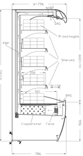
The self-contained vertical ORDC dimensions of the study are 19007961911 mm (LWH). It has four shelves and a well tray (see Figure 1). The experimental study follows the methodology provided by [15] for the test of ORDCs concerning the M-package temperature class M1 (-1 ºC < Tcons < 5 ºC).
a) ORDC configuration and dimensions (mm). b) Test probes locations. Figure 1. Configuration of ORDC and measuring probes locations.
The standard specifies test room climate classes, imposing air temperature, Tamb, and
relative humidity, amb, as well as ambient air movement parallel (amb = 0º) to the
frontal opening plane of the ORDC with a magnitude of vamb = 0.2 m s-1 (henceforth this
for the test room climatic class n.er 3 (Tamb = 25 ºC, amb = 60 %, amb = 0º) but
considering in addition to the ambient air velocity value specified in EN-ISO Standard 23953 (vamb = 0.2 m s-1), the condition when its value is doubled (vamb = 0.4 m s-1). From
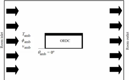
now on this experimental test will be named setup n.er 2. Figure 2 shows the cabinet location and orientation inside the climatic chamber for the experimental setups, in which only the ambient air velocity differs. It also includes the air inlet and outlet of climate chamber.
Figure 2. Experimental setup layout.
The experimental tests were performed inside a climatic chamber Aralab - Fitoclima 650000 EDTU. Figure 1 shows the distribution of test probes inside the ORDC. It was used a data acquisition system Intab PC-Logger 3100 to connect the probes exposed in Table 1. Also in Figure 1 are shown the width of air curtain (bDAG = 60 mm); height of
opening (Hc = 1209 mm); and DAG angle ( = 5º).
n.er Location Type Property Ref.
K-type thermocouple Temperature Tcons
0-4 Conservation
Hygrometer (n.er 1, 3) Relative humidity cons
K-type thermocouple Temperature TDAG
Hot-wire anemometer Velocity vDAG
5 DAG
Hygrometer Relative humidity DAG
K-type thermocouple Temperature TRAG
Hot-wire anemometer Velocity vRAG
6 RAG
Hygrometer Relative humidity RAG
7 Evaporator
(downstream) K-type thermocouple Temperature Tevap_out
8 Evaporator (upstream) K-type thermocouple (contact) Temperature (Surface) Tevap,in 9 Internal surfaces K-type thermocouple
(contact)
Temperature
(Surface) Tsuf
10 Power source Ammeter (clamp-on) Electric current I
Table 1. Description of the test probes and its location.
A probe positioning system is used to evaluate the 3D effects on the thermal entrainment of the re-circulated air curtain and properties variations along length and
height of the conservation space [16]. The probe positioning system was settled in each shelf of the equipment and measured air temperature, relative humidity and velocity for three positions across the air curtain width and eight vertical cross-sections along the equipment's length. The positioning system moved the test probes in 240 mm increments for the 1800 mm length of shelves, taking one minute to move between positions in order to reduce flow perturbation. The parameter values were registed one minute after reaching each position to ensure flow stabilisation. The main procedure followed to accomplish the experimental tests begins with the start up and running of the climatic chamber’s air conditioning system to reach indoor air temperature and relative humidity steady states. Then, the ORDC was loaded with M-packages at proper conservation temperature. The experimental data was collected during 24 hours after M-packages steady state temperatures were accomplished. The average measured values (last 12 hours) of the physical parameters were calculated in order to reduce the experimental results uncertainty, concerning measurements repeatability.
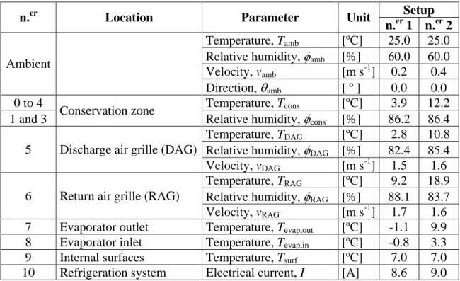
Table 2 shows for each experimental test (setups n.er 1: vamb = 0.2 m s-1 and n.er 2:
vamb = 0.4 m s-1) the average temporal and spatial values of the parameters since they
had been obtained in transient state and for different spatial locations along length.
Setup
n.er Location Parameter Unit
n.er 1 n.er 2
Temperature, Tamb [ºC] 25.0 25.0
Relative humidity, amb [%] 60.0 60.0
Velocity, vamb [m s-1] 0.2 0.4
Ambient
Direction, amb [ º ] 0.0 0.0
0 to 4 Temperature, Tcons [ºC] 3.9 12.2
1 and 3 Conservation zone Relative humidity, cons [%] 86.2 86.4
Temperature, TDAG [ºC] 2.8 10.8
Relative humidity, DAG [%] 82.4 85.4
5 Discharge air grille (DAG)
Velocity, vDAG [m s-1] 1.5 1.6
Temperature, TRAG [ºC] 9.2 18.9
Relative humidity, RAG [%] 88.1 83.7
6 Return air grille (RAG)
Velocity, vRAG [m s-1] 1.7 1.6
7 Evaporator outlet Temperature, Tevap,out [ºC] -1.1 9.9
8 Evaporator inlet Temperature, Tevap,in [ºC] -0.8 3.3
9 Internal surfaces Temperature, Tsurf [ºC] 7.0 7.0
10 Refrigeration system Electrical current, I [A] 8.6 9.0
Table 2. Average values of the parameters measured during the experimental setups. 3 CFD MODELLING
The ORDC model used in this study is a simplified 3D model based on the original one developed by Gaspar et al. [13-14]. The geometry was developed in SolidWorks CAD software, and transferred to Gambit software to build the computational mesh. The CFD code Fluent 6.3.26 was used to simulate the air flow and heat transfer in the ORDC. Since Gaspar et al. [14] made experimental measurements of air velocity, temperature and relative humidity based on this ORDC, the results of the simulation are compared to their experimental results.
The hardware used to run the models was a server with an Intel Xeon DualCore running at 2.33 GHz (4 MBytes internal cache) with 12 GBytes RAM.
3.1 Geometry and computational mesh
The 3D geometry for CFD models closely followed the real one. With the basic size of the model retained, these geometry modifications developed in SolidWorks include resizing food products according to the standard as well as the equipment’s location inside the test room to mimic the ambient air orientation parallel to the ORDC’s frontal opening. The geometry simplifications include removing all curvilinear parts of the cabinet and ignoring inner flow through the internal ducts, across fans and evaporator.
It was used an automatic orthogonal unstructured mesh generator included in Gambit software. The control volume discretization of the refrigerated cabinet and the external surroundings require a computational grid with 1269595 cells and 504368 nodes. The models require such high number of control volumes due to the geometrical distances variations near the end walls of the equipment. This mesh refinement allows the development of a high quality grid without high skewness levels and aspect ratios.
3.2 Mathematical formulation
These governing equations for the averaged flow of an incompressible fluid can be written in the general form by Equation 1 for a dependent variable (= 1 for the continuity equation, = vi , = T, for momentum and energy equations respectively) as
presented by Patankar [17]. is the diffusion coefficient and S represents the source term. S x v xi i (1)
The air is considered as an ideal gas, which state equation relates the parameters of the substance at equilibrium state accurately. The buoyancy-driven forces are treated as a source term in the momentum equations.
The energy equation is developed as a function of temperature in a permanent regime with constant specific heat. Further simplifications are accomplished despising viscous dissipation due to the flow characteristics.
The turbulence was modeled with two equation (one for turbulent kinetic energy and another for dissipation rate of turbulent energy) RNG k- model [18]. Although the RNG k- model is not assumed to be perfectly accurate [19], it’s a good method to simulate turbulence, when the computational capacity is limited. The set of model equations presented above (Equation 1) is suitable for fully turbulent flow. Near the walls, the viscous effects prevail over the turbulent ones. To account for viscous effects and high velocity and temperature gradients in the proximities of the walls, the turbulence model equations are used in conjunction with the empirical wall functions. The complete description and implementation details of the wall functions in turbulence models can be found in Rodi [20] and Launder et al. [21].
The influence of ambient relative humidity is ignored in order to simplify the process of computation. The heat gain of the display case through thermal radiation by surrounding heat sources is not considered due to the computation time and CPU-intensive calculation. These simplifications are considered for the engineering approximation models.
3.3 Numerical model
The mathematical model is a set of coupled non-linear partial differential equations, expressing mass, momentum and energy conservation which should be simultaneously
and interactively solved. The computational procedure applied is based on a numerical iterative process using the Coupled algorithm for the pressure-velocity coupling. It solves the momentum and pressure-based continuity equations together. The full implicit coupling is achieved through an implicit discretization of pressure gradient terms in the momentum equations, and an implicit discretization of the face mass flux, including the Rhie-Chow pressure dissipation terms [22-23]. This algorithm increases CFD robustness and reduces computation time although it needs more memory requirements [24-25]. The equations were discretized in the control volume form using the MUSCL (Monotone Upstream-Centered Schemes for Conservation Laws) differencing scheme. The MUSCL scheme proposed by Van Leer [26] relies on the Central Differencing Scheme (CDS) and on the Second Order Upwind (SOU) differencing scheme) [17]. It is a differencing scheme with higher spatial precision for all types of computational grids and for complex flows, since it reduces the numerical diffusion. Due to convergence difficulties, the First Order Upwind differencing scheme (FOU) was used to discretize the turbulent quantities [17].
3.4 Boundary conditions
The results of this work can be compared with those of Gaspar et al. [13], as most of the boundary conditions (BCs) have been assumed to be the same. The BC imposed on the computational domain are those of common practice in numerical simulations, defined for the climatic class n.er 3 of EN-ISO Standard 23953 [15] (Tamb = 25 ºC, amb
= 60 %). However, there are differences at the inlet and at the outlet boundary conditions. Also, for several models and simulations, the boundary conditions of DAG, RAG and PBP are different.
Inlet boundary conditions
DAG is simulated by a flow inlet BC where the experimental average values of temperature and velocity for each setup are specified (see Table 1).
The values of air temperature and velocity of climate class n.er 3 are imposed at the room inlet.
The mass flow rate at PBP, mPBP, is determined by mass conservation: DAG RAG PBP out in m m m m m (2)
The temperature of the air flowing through the PBP is assumed to follow the least squares of the third order polynomial of air temperature evolutions at DAG and downstream the evaporator due to the values similarity with experimental measurements.
The turbulence parameters for each flow inlet BC are specified in terms of hydraulic diameter, Dh, and turbulence intensity, It, like expressed by Equation 3.
Re
18 16 . 0 h D t I (3) Outlet boundary conditions
Outlet BCs are specified at RAG and room outlet. The values specified for each setup at RAG are based on experimental average values (see Table 1).
The value of air velocity of climate class n.er 3 leaving the computational domain is imposed at the room outlet. The turbulence parameters are specified as for inlet BCs.
Heat flux boundary conditions
The walls not considered in heat transfer calculus are assumed as adiabatic BC. However, the heat flux BC is used to simulate the heat generated by illumination (85% for fluorescent lamp) and the heat flux through conduction across material layers that compose the walls of the equipment. The conduction heat fluxes are specified as BC (see Table 3), using the Fourier Law with a global heat transfer coefficient based on conductive thermal resistances of each wall material. The experimental temperature values of the interior and exterior surfaces of the equipment are used. These BCs are the same in all setups.
Surfaces Variable Unit Value
Illumination (OSRAM L58W/20) qilum W m
-2
10.00
Top qduct,top W m-2 6.08
Rear qduct,rear W m
-2
7.63 Interior surfaces of the equipment
Down qduct,down W m
-2
6.96
Table 3. Walls heat flux boundary condition.
Wall boundary condition
Wall BCs are used to bound fluid and solid regions. At the walls a non-slip BC is considered. For the surfaces of the plastic sheet (polipropylene) that enclosure the food product is imposed a thin-wall BC to solve the heat conduction equation, computing the thermal resistance of the plastic. The values are: = 912 kg m-3; specific heat: Cp = 1.94 kJ kg-1 K-1; thermal conductivity: k = 0.25 W m-1 K-1; and thickness: = 25.410-6
m.
Product load (solid region)
Based on the EN-ISO standard 23953 [15], the product simulators are made of tylose, whose thermal characteristics are similar to meat. Its equivalent solid thermal characteristics are imposed considering the values given by ASHRAE [27].
3.5 Solution monitoring and control techniques
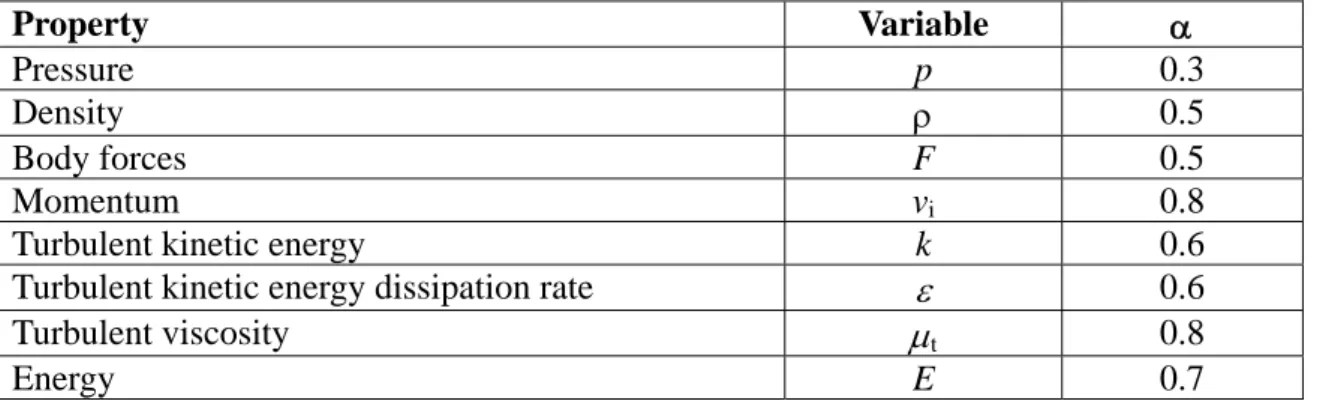
The linear relaxation method is used to reduce the high variation of dependent variables during the iterative process. Table 4 shows values of linear relaxation factors,
, for the scalar and vector quantities.
Property Variable
Pressure p 0.3
Density 0.5
Body forces F 0.5
Momentum vi 0.8
Turbulent kinetic energy k 0.6
Turbulent kinetic energy dissipation rate 0.6
Turbulent viscosity t 0.8
Energy E 0.7
The convergence monitoring process evaluates the sums of absolute residuals of mean field variables. Each simulation reaches the convergence criterion (required
110-6
for all residuals) after 2500 iterations. To obtain an optimal comparison between the different simulations, they have been stopped at 2500 iterations.
4 RESULTS AND DISCUSSION
The influence of ambient air velocity magnitude on the thermal behaviour of the ORDC is evaluated analyzing both experimental results and 3D numerical predictions of the CFD parametric study considering the air movement parallel to the equipment’s frontal opening plane with velocity values of 0.2 m s-1 (setup n.er 1) and 0.4 m s-1 (setup n.er 2)
4.1 Comparison with experimental data
The validation of numerical results is accomplished by its comparison with experimental measurements data obtained by Gaspar et al. [13]. The predicted steady state air flow and heat transfer inside ORDC present both a reasonable quantitative agreement and a qualitative similar trend, being the highest quantitative discrepancy in the proximity of air curtain. Considering air temperature and velocity variation drifts measured during experimental testing, the global average relative deviation between experimental data and numerical predictions of air temperature and velocity are acceptable in engineering situations. The non-overlapping of results (experimental and numerical) is due to experimental errors (measurements precision, physical phenomena perturbation, etc) and computational model assumptions (steady state, turbulence model, boundary conditions definition, etc). Nevertheless, the combined analysis of experimental and numerical results shows that the CFD model generally follows the pattern of the physical phenomena occurring in the real equipment.
4.2 Thermal entrainment factor calculation
The thermal performance of an ORDC taking into account the thermal barrier provided by the air curtain, is evaluated by the thermal entrainment factor (TEF) without PBP air flow, X0, calculation as proposed by [3, 8, 10] and defined in Equation
4. The TEF will be zero if there is no entrainment: hRAG = hDAG (unreachable condition)
and it will increase with air enthalpy at RAG. When return air is only from the surrounding ambient air, hRAG = hamb, the thermal entrainment factor will reach unity.
These studies considered the thermal entrainment factor expressed through temperatures, i.e., assuming the specific heat capacity of air, Cp, to be constant.
DAG amb DAG RAG DAG amb DAG RAG 0 T T T T h h h h X (4)
Yu et al. [27] deducted the TEF formula with PBP airflow (Equation 5) based on
TEF without PBP airflow.
PBP 0 0 ) 1 ( X X X TEF (5)
Where is the PBP airflow ratio given by:
DAG PBP PBP m m m (6)
And XPBP is the TEF for PBP airflow: DAG amb DAG PBP PBP T T T T X (7)
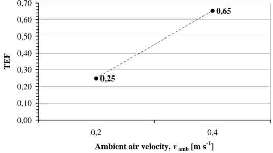
The TEF results from the experimental setups calculated with the average air
enthalpies show that the infiltration heat transfer rate is dependent on the magnitude of ambient air velocity, vamb. The TEF trend with the ambient air velocity magnitude is
shown in Figure 3. The increase of ambient air velocity value from 0.2 m s-1 to 0.4 m s-1 increases TEF almost three times. This means a very low thermal behaviour and performance of the ORDC.
0,25 0,65 0,00 0,10 0,20 0,30 0,40 0,50 0,60 0,70 0,2 0,4
Ambient air velocity, vamb [m s -1
]
TEF
Figure 3. Comparison of TEF calculation for different ambient air velocity magnitude. 4.3 Numerical predictions
The numerical simulations allow the analysis of air temperature and velocity distributions within the equipment to evaluate its thermal behaviour dependence of ambient air velocity magnitude.
Temperature fields along y-z
Figure 4 presents the temperature maps for selected vertical planes along length for each setup. Sections x/L = 0.03 and x/L = 0.97 are vertical planes near the equipment’s lateral walls. The temperature fields show the influence of the ambient air velocity magnitude on the aerothermodynamic performance of the air curtain and on the air temperature distribution inside the conservation space. It is shown that the equipment’s end walls promote air curtain instability and thus thermal entrainment. The numerical predictions indicate refrigerated air losses to the exterior by the bottom part of the equipment (near RAG) in both setups.For setup n.er 1 (vamb = 0.2 m s-1), the air curtain
instabilities are more significant at the left side (x/L = 0.03), i.e., the side from the ambient air comes in. Air leakage is much more obvious in setup n.er 2 (vamb = 0.4 m s-1)
which presents nearly no air curtain. One reason for much more air leakage near the lateral wall is that the ambient air entering parallel to the frontal opening causes both intense turbulence and vortex formation near the lateral wall than in other ambient air directions. However, comparing the setups’ sections, setup n.er 1 presents always better
thermal behaviour (lower average values of air and product temperatures). This condition is due to lower thermal entrainment across air curtain in middle length of the frontal opening plane than in other setup.
a1) section x/L = 0.03. b1) section x/L = 0.97. Setup n.er 1 (Ambient air velocity: vamb = 0.2 m s-1).
a2) section x/L = 0.03. b2) section: x/L = 0.97. Setup n.er 2 (Ambient air velocity: vamb = 0.4 m s-1).
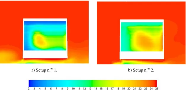
Temperature fields in air curtain plane
Figure 5 shows for each setup the air temperature fields for a vertical plane between DAG and RAG width middle sections. These numerical results show where the thermal entrainment is higher and how it spreads across air curtain. Considering that the air movement is mainly from left to right on figures a) and b) (setups n.er 1 and n.er 2), the vortex formation occurs after overcome the equipment’s lateral wall, increasing the thermal entrainment as the equipment's length increases. Nevertheless, air vortex occurs mainly near equipment’s extremities as is shown in figure. Setup n.er 1 presents comparably good thermal conservation with lowest temperature and slight vortex. It also can be seen that for setup n.er 2, the temperature average value prediction in the vertical plane between DAG and RAG is much higher than in other setup.
a) Setup n.er 1. b) Setup n.er 2.
Figure 5. Air temperature field maps, T [ºC], for a vertical plane between DAG and RAG width middle sections.
Temperature fields along x-y
Figure 6 presents the air temperature fields in x-y planes at different heights from RAG (z/H = 0.38) to DAG (z/H = 0.92) for each setup. For all setups, the air temperature numerical predictions at the air curtain interface show the air curtain stability increase with height. The air curtain is well defined along length (x/L) near the DAG (z/H = 0.92) for setup n.er 1. Setup n.er 2 presents nearly no air curtain close to RAG, resulting in air vortex for most part of the conservation zone.
As the air curtain height increases (< z/H), it can be observed that the thermal entrainment increases near the end walls for setups n.er 1 and n.er 2 and across the air curtain for all setups. The air turbulence predictions are very intense on the section close to RAG for both setups.
The ambient air direction is parallel relatively to the equipment’s frontal opening, promoting air vortices (visible in temperature fields by the mixture that is triggered) mostly near the area where the ambient air enters. Comparing the temperatures of two setups, obviously setup n.er 1 presents the lowest product temperature, thus the best food preservation.
The ambient air velocity near the re-circulated air curtain for all setups show an obvious increase than other areas, indicating intense turbulence near air curtain.
The numerical results show a higher influence of the ambient air movement (from top to down in figure 6) in the dimension of eddies structures located near the equipment’s end walls.
In figure 6 b1) and b2), it can be observed that between 2nd and 3rd shelves (z/H = 0.66), setups n.er 1 and n.er 2 still present air vortexes, of which the later is more intense.
c1) c2) Near DAG (z/H = 0.92).
b1) b2) Middle height between 2nd and 3rd shelves (z/H = 0.66).
a1) a2) Near RAG (z/H = 0.38).
Setup n.er 1. Setup n.er 2.
Figure 6. Air temperature field maps, T [ºC], along equipment’s non dimensional height, z/H.
Globally, it can be observed that the temperature between shelves presents obvious differences among setups, indicating that based on the same condition, the setup in which ambient air velocity has lower value presents better thermal behaviour.
As the ambient air velocity increases, there is a reduction of the air curtain aerothermodynamics performance.
The non uniformity of the refrigerated air temperature distribution along the spatial coordinates influences the food temperature differences depending on their location in the shelves.
5 CONCLUSION
A 3D CFD parametric study applied to an open refrigerated display cabinet has been developed to evaluate the influence of the ambient air velocity in the equipment’s thermal behaviour. The characterization of air flow and heat transfers allows the identification of equipment’s length impact in thermal entrainment. The thermal entrainment downward the air curtain is very dependent of the eddies formation that increases with the ambient air velocity magnitude. Eddies are developed by shear layer interactions and enhanced by turbulence intensity at the initial region of the air curtain jet that triggers mixture. The momentum reduction decreases the re-circulated air curtain stability as its distance from discharge air grille increases. The numerical results analysis revealed high values of the thermal entrainment at the initial and final linear dimensions due to side wall effects for setups. When the magnitude of the ambient air velocity is doubled (vamb = 0.4 m s-1), the thermal entrainment occurs at all length and
height of air curtain, being more significant at lower height due to momentum reduction of air curtain.
As the ambient air velocity increases, its influence on the thermal behaviour increases. These conditions will promote a non-uniform air temperature distribution inside the refrigerated display cabinet and influences variations in the product temperature. Additionally, the ambient air movement affects the return air temperature and consequently the energy efficiency of the equipment.
To optimize the thermal behaviour of open refrigerated display cabinets is required to select the optimum discharge air velocity, but also to ensure that the room conditions where the fixture will be installed take into account a location away from air conditioning system discharge grilles, reduced air mass flows originated by pressure differences due to openings to surroundings, among others.
NOMENCLATURE General Cp Specific heat, [J kg-1 K-1]. Dh Hydraulic diameter, [m]. F Force, [N]. h Entalpy, [J/kg]. H Height, [m].
I Electrical current, [A].
It Turbulence intensity, [%].
k Turbulent kinetic energy, [m2 s-2]; Thermal conductivity, [W m-1 K-1].
L Length, [m].
m Mass flow rate, [kg s-1].
p Pressure, [Pa].
q Heat flux, [W m-2].
Re Reynolds number.
S General source term.
T Temperature, [ºC].
v Average velocity, [m s-1].
W Width, [m].
x, y, z Spatial coordinates, [m].
X0 Thermal Entrainment Factor (without PBP airflow).
XPBP Thermal Entrainment Factor for PBP airflow.
Superscripts and subscripts amb Ambient. cons Conservation. DAG Discharge air grille. evap Evaporator.
i Index. ilum Illumination. in input. out Output. PBP Perforated back panel. prod Product.
RAG Return air grille. surf surface. Greek Symbols
Linear relaxation factor. PBP airflow ratio.
Thickness, [m].
Dissipation rate of k, [m2 s-3].
Relative humidity, [%]; General variable.
Convergence criterion. Dynamic viscosity, [kg m-1 s-1]. Angle, [ º ]. Density, [kg m-3]. Diffusion coefficient. Acronyms 2D Two-dimensional. 3D Three-dimensional. BC Boundary condition.
CAD Computer Aided Design. CDS Central Differencing Scheme. CFD Computational Fluid Dynamics. CPU Central Processing Unit.
DAG Discharge air grille.
FOU First Order Upwind.
MUSCL Monotone Upstream-Centered Schemes for Conservation Laws. ORDC Open Refrigerated Display Cabinet.
PBP Perforated back panel.
RNG Renormalization Group Theory.
SOU Second Order Upwind.
RAG Return air grille.
ACKNOWLEDGMENTS
The authors wish to acknowledge the support of University of Beira Interior – Engineering Faculty – Electromechanical Engineering Department and of the refrigerated display cabinet manufacturer JORDÃO Cooling Systems®, Guimarães, Portugal (www.jordao.com). Thanks also to the IAESTE (International Association for the Exchange of Students for Technical Experience) and FCT (Fundação para a Ciência e a Tecnologia) for the support of post-graduate students.
REFERENCES
[1] ASHRAE, 2006 ASHRAE Handbook: Refrigeration, American Society of Heating, Refrigerating and Air-Conditioning Engineers Inc, (2006).
[2] R. Faramarzi, Efficient display case refrigeration. ASHRAE Journal 41(11) (1999). [3] Y.-G. Chen and X.-L. Yuan, Experimental study of the performance of single-band air curtains for multi-deck refrigerated display cabinet. J. Food Engineering 69(3), pp. 261-267 (2005).
[4] I. Gray et al., Improvement of air distribution in refrigerated vertical open front remote supermarket display cases. Int. J. Refrigeration 31(5), pp. 902-910 (2008).
[5] G. Cortella, M. Manzan and G. Comini, CFD simulation of refrigerated display cabinets. Int. J. Refrigeration 24(3), pp. 250-260 (2001).
[6] H.K. Navaz, R. Faramarzi, M. Gharib, D. Dabiri and D. Modarress, The application of advanced methods in analyzing the performance of the air curtain in a refrigerated display case. Trans. ASME J. Fluids Eng. 124, pp. 756–764 (2002).
[7] M. Axell and P. Fahlén, Design criteria for energy efficient vertical air curtains in display cabinets, In proceedings of 21st IIR Int. Congress of Refrigeration, Washington DC, U.S.A. (2003).
[8] H.K. Navaz, B.S. Henderson, R. Faramarzi, A. Pourmovahed and F. Taugwalder, Jet entrainment rate in air curtain of open refrigerated display cases. Int. J. Refrigeration
28(2), pp. 267-275 (2005).
[9] A.M. Foster, M. Madge and J.A. Evans, The use of CFD to improve the performance of a chilled multi-deck retail display cabinet. Int. J. Refrigeration 28(5), pp. 698-705 (2005).
[10] P. D’Agaro, G. Cortella and G. Croce, Two- and three-dimensional CFD applied to vertical display cabinets refrigeration. Int. J. Refrigeration 29(2), 178-190 (2006).
[11] Y.-G. Chen, Parametric evaluation of refrigerated air curtains for thermal insulation. Int. J. Thermal Sciences 48(10), pp. 1988-1996 (2009).
[12] Y.T. Ge and S.A. Tassou, Simulation of the performance of a single jet air curtains for vertical refrigerated display cabinets. Int. J. Refrigeration 21(2), pp. 201–209 (2001).
[13] P.D. Gaspar, L.C.C. Gonçalves and X. Ge, Influence of ambient air velocity orientation in thermal behaviour of open refrigerated display cabinets. In proceedings of the of the ASME 2010 10th Biennial Conference on Engineering Systems Design and Analysis, ESDA2010, July 12-14, 2010, Istanbul, Turkey (2010).
[14] P.D. Gaspar, L.C.C. Gonçalves and R.A. Pitarma, Three-dimensional CFD modelling and analysis of the thermal entrainment in the open refrigerated display cabinets. In proceedings of the 2008 ASME Summer Heat Transfer Conference, Jacksonville, U.S.A. (2008).
[15] EN-ISO Standard 23953, Refrigerated display cabinets, parts 1 and 2. ISO - International Organization for Standardization (2005).
[16] P.D. Gaspar, L.C.C. Gonçalves and R.A. Pitarma, Experimental analysis of the thermal entrainment three dimensional effects in recirculated air curtains. In proceedings of 10th Int. Conf. on Air Distribution in Rooms – ROOMVENT 2007, Helsinki, Finland (2007).
[17] S.V. Patankar, Numerical Heat Transfer and Fluid Flow. Hemisphere Publishing Corporation (1980).
[18] V. Yakhot and S.A. Orszag, Renormalization Group Analysis of Turbulence: I. Basic Theory. J. of Scientific Computing 1(1), pp. 3-51 (1986).
[19] N.J. Smale, J. Moureh and G. Cortella, A review of numerical models of airflow in refrigerated food applications. Int. J. Refrigeration 29(6), pp. 911-930 (2006).
[20] W. Rodi, Turbulence models and their application in hydraulics. A state of the art review. International Association for Hydraulics Research (1980).
[21] B.E. Launder and D.B Spalding, The numerical computation of turbulent flows. Computer Methods in Applied Mechanics and Engineering 3(2), pp. 269-289 (1974). [22] Fluent, Fluent 6.3 User’s Guide. Fluent Inc. (2006).
[23] Fluent, Fluent 6.3 Theory Guide. Fluent Inc. (2006). [24] Ansys, ANSYS Advantage II(2). Ansys (2008).
[25] F. Moukalled and M. Darwish, A coupled finite volume solver for incompressible flows: Numerical analysis and applied mathematics, In proceedings of International Conference on Numerical Analysis and Applied Mathematics AIP 2008, Vol. 1048, pp. 715-718 (2008).
[26] B. Van Leer, Toward the ultimate conservative difference scheme, IV, a second order sequel to Godunov's method. J. of Computational Physics 32(1), pp. 101-136 (1979).
[27] ASHRAE, ASHRAE Handbook: Fundamentals, American Society of Heating, Refrigerating and Air-Conditioning Engineers Inc. (1997).
[28] K.-Z. Yu, G.-L. Ding and T.-J. Chen, A correlation model of thermal entrainment factor for air curtain in a vertical open display cabinet. Applied Thermal Engineering
![Figure 4. Air temperature field maps, T [ºC], along equipment’s non dimensional length, x/L](https://thumb-eu.123doks.com/thumbv2/123dok_br/18081202.865537/11.892.131.763.185.581/figure-air-temperature-field-along-equipment-dimensional-length.webp)
![Figure 6. Air temperature field maps, T [ºC], along equipment’s non dimensional height, z/H](https://thumb-eu.123doks.com/thumbv2/123dok_br/18081202.865537/13.892.120.775.247.1003/figure-air-temperature-field-maps-equipment-dimensional-height.webp)
