Income inequality, TFP, and human capital

(1)

Repositório ISCTE-IUL

Deposited in Repositório ISCTE-IUL:

2019-03-22

Deposited version:

Post-print

Peer-review status of attached file:

Peer-reviewed

Citation for published item:

Sequeira, T. N., Santos, M. & Ferreira-Lopes, A. (2017). Income inequality, TFP, and human capital. Economic Record. 93 (300), 89-111

Further information on publisher's website:

10.1111/1475-4932.12316

Publisher's copyright statement:

This is the peer reviewed version of the following article: Sequeira, T. N., Santos, M. & Ferreira-Lopes, A. (2017). Income inequality, TFP, and human capital. Economic Record. 93 (300), 89-111, which has been published in final form at https://dx.doi.org/10.1111/1475-4932.12316. This article may be used for non-commercial purposes in accordance with the Publisher's Terms and Conditions for self-archiving.

Use policy

Creative Commons CC BY 4.0

The full-text may be used and/or reproduced, and given to third parties in any format or medium, without prior permission or charge, for personal research or study, educational, or not-for-profit purposes provided that:

(2)

For Review Only

Income Inequality, TFP, and Human Capital

Journal: The Economic Record

Manuscript ID ECOR-2016-057.R1

Manuscript Type: Original Research

Keywords: income inequality, human capital, technology

(3)

For Review Only

Income Inequality, TFP, and Human Capital

Abstract

A fruitful recent theoretical literature has related human capital and technological development with income (and wages) inequality. However, empirical assessments on the relationship are relatively scarce. We relate human capital, total factor productivity (TFP), and openness with inequality and discover that, when countries are assumed as heterogeneous and dependent cross-sections, human capital is the most robust determi-nant of inequality, contributing to increase inequality, as predicted by theory. TFP and Openness revealed to be non significantly related to inequality. These results are robust to a number of robustness tests on specifications and data and open prospects for theo-retical research on the country-specific features conditioning the effect of human capital, technology and trade on inequality.

JEL Codes: I24, I32, O10, O33, O50. 1 2 3 4 5 6 7 8 9 10 11 12 13 14 15 16 17 18 19 20 21 22 23 24 25 26 27 28 29 30 31 32 33 34 35 36 37 38 39 40 41 42 43 44 45 46 47 48 49 50 51 52 53 54 55 56 57

(4)

For Review Only

1 Introduction

Understanding the causes of inequality is fundamental to indicate possible policy measures that ensure that the increased production and income of societies can be better shared among the whole population. Reducing inequality is important not just to achieve a fairer distribution of income and address the social concerns that widening disparities in income raise, but also to ensure a good environment for growth. As has been seen in some countries, these social concerns can lead to social instability. Income inequality may itself limit the growth potential of economies as social, economic, and political instability caused by inequality is associated with slower growth. Even in democracies, an increase in inequality may contribute to elect politicians that are against openness and globalization, which may deter the world integration process which is known to have positive effect on the growth prospects of the economy.

This paper contributes to our knowledge of the relationship between human capital, tech-nology and inequality in two crucial ways: first, it uses a large database on inequality, based on the Standardized World Income Inequality dataset, and combines it with the most recent data for human capital and TFP to explain cross-country patterns of inequality; second, for the first time, it takes into account country heterogeneity, cross-country dependence, and endogeneity to common factors in evaluating the effects of human capital and TFP on inequality. The exploration of a large dataset of over 150 countries across more than 50 years (since 1960) al-lowed us to explore issues such as panel heterogeneity, cross-country dependence and time-series features, such as stationarity and causality, which are absent from earlier contributions.

There is a fruitful theoretical literature interested in explaining the rise of inequality in the second-half of the twentieth century (mainly in the USA) together with the rise in the supply of human capital. Skill biased technical change and capital-skill complementarity have been crucial to explain this phenomenon. Generally, according to this theory, skill-premia increase due to two effects. First, the skill premium would reflect the productivity difference between sectors. Second, with full capital mobility, factor price equalization requires capital to flow to the sector operating the new technology, and thus workers in the new technologies sectors are

1 2 3 4 5 6 7 8 9 10 11 12 13 14 15 16 17 18 19 20 21 22 23 24 25 26 27 28 29 30 31 32 33 34 35 36 37 38 39 40 41 42 43 44 45 46 47 48 49 50 51 52 53 54 55 56

(5)

For Review Only

endowed with more capital, which boosts their relative wages (Acemoglu, 2002a, 2002b, 2003). An alternative development has argued that the diffusion of IT - General Purpose Technologies - may have raised the demand for adaptable skilled workers and made vintages of capital more adaptable. Therefore, this increases the premium of workers that show a lower learning cost and can adapt quickly from one sector to another. These ideas have been formalized by Galor and Tsidon (1997), Greewood and Yorukoglu (1997), Caselli (1999), Galor and Moav (2000) and Aghion, Howitt, and Violante (2002). Theoretically, skill-biased technological change is explained by the proportion of skills (education) in the economy, and wage inequality (typically measured by the wage ratio between skilled and unskilled workers) is proportional to the proportion of skills in the economy. Education is thus seen in the theory as a determinant of more technical change (and consequently growth) and more inequality.

Whatever the explanation is for the rise in inequality and its relationship to technology and human capital, there is little quantitative literature on the issue, as pointed out by Hornstein, Krusel and Violante (2005:1361). In fact, empirical attempts to evaluate the relationship are mostly country-specific as, e.g. Ding et al. (2011) and Rattsø and Stokke (2013) dealing with the effect of technology, and in Birchenall (2001) dealing with the effect of human capital. Micro evidence on the relationship between education and income inequality is mixed. While Martins and Pereira (2004) found a positive sign for the effect of education returns in inequality due to an increase in returns to education throughout the wage distribution for 16 European Countries, Wang (2011) found returns to education in China that are more pronounced for individuals in the lower tail of the earnings distribution than for those in the upper tail, in stark contrast to the results found in some developed countries.

We have found a handful of papers that evaluated this relationship using a large cross-section of countries. Some of these papers are solely concerned with the relationship between education and inequality. Milanovic (2000) reassessed the Kuznets (1955) initial contribution, adding institutional variables to the analysis of determinants of the income inequality. Teulings and van Rens (2008) found evidence for a negative relationship between increase in schooling and returns in a cross-section of countries, implying a contribution of schooling to reduce

1 2 3 4 5 6 7 8 9 10 11 12 13 14 15 16 17 18 19 20 21 22 23 24 25 26 27 28 29 30 31 32 33 34 35 36 37 38 39 40 41 42 43 44 45 46 47 48 49 50 51 52 53 54 55 56 57

(6)

For Review Only

inequality, a result that goes on the same direction that the obtained by Gregorio and Lee (2002).

Three other papers relate income inequality in cross-sections with several controls, among which particular attention is given to education,technology, openness and institutions. Barro (2000) presents fixed-effects estimations of equations of the Gini index on covariates such as GDP and GDP squared, schooling, democracy index, openness, rule of law index and several dummies. In his fixed-effects estimations, dummies for income or spending and secondary schooling are negatively related to inequality and higher schooling and openness are posi-tively related to inequality (with significant coefficients). Primary schooling and the dummy for individual or household data are insignificantly related to the Gini coefficient. There is a strong inverted-U relationship with GDP (the so-called Kuznets curve) in Barro’s estimations. Rodriguez-Pose and Tselios (2009) present positive and robust signs for secondary and tertiary education levels and income inequality among European regions. Additionally, these authors found that population ageing, female participation in the labor force, urbanization, agricul-ture, and industry are negatively associated to income inequality, while unemployment and a specialization in the financial sector positively affect inequality. Finally, income inequality is lower in social-democratic welfare states, in Protestant areas, and in regions with Nordic family structures. Recently, Jaumotte, Lall, and Papageorgiou (2013) re-assessed the determinants of inequality. They focus on the effect of globalization on inequality but avoid the relation-ship between inequality and GDP. They conclude that trade globalization decreases inequality while financial globalization increase inequality. Moreover, information and communication technologies and credit deepening increases inequality while the share of industry in the econ-omy decreases inequality. Interestingly, education variables and initial GDP (when included) are insignificantly related to inequality.

As can be noted, empirical evidence coming from a large cross-section of countries has quite ambiguous results regarding the determinants of inequality and does not confirm theories in crucial aspects such as the influence of education and technology. However, much criticism has affected data on inequality around the world. In fact, greater coverage across countries and

1 2 3 4 5 6 7 8 9 10 11 12 13 14 15 16 17 18 19 20 21 22 23 24 25 26 27 28 29 30 31 32 33 34 35 36 37 38 39 40 41 42 43 44 45 46 47 48 49 50 51 52 53 54 55 56

(7)

For Review Only

over time is available from these sources only at the cost of significantly reduced comparability across observations. There are currently three different projects that collect and make publicly available inequality data for many countries and periods around the world: the Luxembourg Income Study (LIS), the dataset assembled by Deininger and Squire (1996) for the World Bank (WIID) - recently updated and upgraded by the WIDER (World Institute for Development Economic Research) project, and the most recent standardized World Income Inequality dataset (SWIID), by Solt (2009). The LIS, which was used by Jaumotte, Lall, and Papageorgiou (2013), has generated the most-comparable income inequality statistics currently available but covers relatively few countries and years. The Deininger and Squire dataset and its successors, used by Barro (2000), on the other hand, provide much more observations, but only at a substantial loss of comparability. Solt (2009) implemented a sequence of steps in order to standardize income inequality data and provide data with more ample coverage than the WIID but at the highest quality as in LIS. However, in the process of standardization, not all countries had the sufficient data in the original sources. To handle this, Solt (2009) also calculated a standard-error of each Gini coefficient to account for the remaining uncertainty in data. The disadvantage of using cross-country data is that it may ignore some micro effects that can be studied in micro-data. The interesting feature of inequality data however and it is based in country micro studies on inequality. Exploring the heterogeneity of data concerning the determinants of inequality is especially important since the effects of different inequality determinants may differ considerably from country to country. In fact, and to give a few examples, the effect of technology adoption may differ if the country is on the technological frontier or lagging behind; the effect of human capital may differ between countries where brain-drain is more evident than in others; and the effect of openness may depend crucially on the level of integration and on the market size of the country. In general, historical and institutional (e.g. labor market related) country-specific factors that are not simply captured by fixed-effects estimations, are in fact dealt through heterogeneous panel estimations.

Our main conclusions point out to a clearly significant, worldwide relevant, positive effect of human capital on inequality, an effect that is stronger for the developed world. On the contrary,

1 2 3 4 5 6 7 8 9 10 11 12 13 14 15 16 17 18 19 20 21 22 23 24 25 26 27 28 29 30 31 32 33 34 35 36 37 38 39 40 41 42 43 44 45 46 47 48 49 50 51 52 53 54 55 56 57

(8)

For Review Only

our results indicate that the effects of technology and openness are not statistically significant, as well as dependent on different specifications. Overall, the common factors framework dismiss the existence of a Kuznets curve.

The remainder of the paper is organized as follows. Next, in Section 2 we describe our dataset. In Section 3 we describe our estimation strategy. In Section 4 we present our results, beginning with detailed evidence for cross-country dependence, stationarity, and evidence of (Granger-) causality and then showing the results from several different specifications based on heterogeneous panels methods. Section 5 concludes.

2 Sources and Data

We use data from the Standardized World Income Inequality database (SWIID), version 4.0, from Solt (2009), for the Gini coefficient.1,2 _{These include data on the Gini coefficient using}

post-taxes and post-transfers income (the net definition) and on the Gini coefficient using pre-taxes and pre-transfers income (the market definition), and the respective standard-errors by country and year. Previous data on inequality have presented variables divided by the type of underlying measure of inequality (income or consumption) and by the quality of data (e.g. defining different quality levels). Solt (2009) maintained the same concerns within their dataset. He divides data in net and market Gini indexes which may be roughly matched with consumption and (net) income Gini indexes, by one side, and (gross) income Gini indexes, by the other side. Additionally they provide the data with a standard-deviation, which intends to measure uncertainty in data, basically due to less availability of underlying data to calculate inequality measures in some countries. Thus, this can be interpreted as the information about

1_{Available at http : //thedata.harvard.edu/dvn/dv/fsolt/faces/study/StudyP age.xhtml?studyId =}

36908. This is the first time this source for inequality data is used to access the relative importance of the determinants of inequality. We explained above the reasons why this choice is superior to the previously used data.

2_{In a working-paper version of this article, we compare some results with inequality data coming from}

the Word Income Inequality database (WIID2c). In doing so, we followed some strict criteria to select data, separating Gini coefficients from net income, consumption and gross income and preferring data with wide coverage and higher quality. In that analysis, we also made clear that SWIID have more than four times the number of observations than the measures coming from the WIID, making SWIID more suitable (if not the unique suitable) for being studied with heterogeneous panel data methods.

1 2 3 4 5 6 7 8 9 10 11 12 13 14 15 16 17 18 19 20 21 22 23 24 25 26 27 28 29 30 31 32 33 34 35 36 37 38 39 40 41 42 43 44 45 46 47 48 49 50 51 52 53 54 55 56

(9)

For Review Only

the quality of the underlying data. In the majority of the analysis made in the paper, we will use a quality-adjusted measure of the SWIID gini coefficient which is simply given by dividing the Gini coefficient by the respective standard-deviation, provided by Solt (2009).3

We use GDP per capita, openness, human capital index, and TFP index from Penn World Tables (PWT), version 8.0 (Feenstra et al., 2013).4 _{Human capital in PWT 8.0 is measured}

by a ‘Mincerian’ combination of years of schooling (from Barro and Lee, 2013, version 1.3) and returns to education. The results from Psacharopoulos (1994) show that returns from schooling decrease across years of schooling. As the influence of human capital in inequality arguably changes through years of schooling (Barro’s results show negative signs for primary and secondary schooling and positive signs for tertiary schooling) and returns from schooling are essential to understand income inequality, we think this variable is the most appropriate human capital measure to enter in inequality regressions. In fact, as human capital measures corrected for returns for education weights more lower levels of education, they correct un-derestimations of human capital in less developed countries. Lower levels of education in less developed countries may have more influence in decreasing wage inequality than they have in more developed countries. The human capital measure provided by the PWT 8.0 is the one with the highest coverage until now, as it not only corrects years of schooling by different re-turns by levels of education, but it is also interpolated to provide annual measures. It is worth noting that returns to education differ between levels of education but not between different countries or years as these alternatives would result in lower coverage.

TFP is available in PWT 8.0 both as a ratio to the USA=1 level and on constant national prices. We construct our index departing from a final TFP level (related to the USA) in 2011 and then deflating year by year using growth rates of the national currency measure of TFP. This allows us to have a PPP measure of TFP that is independent of the USA level (at an

3_{The uncertainty-corrected measure is} GIN I

sd(GIN I), where GINI is the Gini index provided by SWIID and

sd(GINI) is the standard-deviation of the Gini index, also provided by the SWIID and that corrects for un-certainty or measurement error within the sources. Later on, on the Discussion section, we discuss the results obtained with an alternative uncertainty-corrected measure.

4_{Available at http : //www.rug.nl/research/ggdc/data/penn − world − table.}

1 2 3 4 5 6 7 8 9 10 11 12 13 14 15 16 17 18 19 20 21 22 23 24 25 26 27 28 29 30 31 32 33 34 35 36 37 38 39 40 41 42 43 44 45 46 47 48 49 50 51 52 53 54 55 56 57

(10)

For Review Only

Table 1: Descriptive Statistics

Variable N. Obs Mean Std. Dev. Min Max

Gini (net) 4597 3.5923 0.2960 2.7324 7.3871

Gini (market) 4597 3.7395 0.2234 2.8367 4.3740

Gini (net) - value/sd 4597 3.5613 0.9786 1.2658 9.5894

Gini (market) - value/sd 4597 3.2479 1.0049 1.0747 9.5410

Human Capital 6797 0.6905 0.3160 0.0198 1.2861

TFP 4994 0.5254 0.5287 -3.5389 1.1222

Openness 7760 1.1645 1.1020 -12.7415 3.2061

GDP per capita 7760 8.2779 1.1891 4.8890 10.9961

Notes: Gini variables are from SWIID - Standardized World Income Inequality Database, from Solt (2009). In the source, Gini variables are measured from 0 to 100 (in percentage). Human Capital, TFP, Openness = (Exports+Imports)/GDP - and GDP per capita are from PWT 8.0. When value/sd is indicated it means that the Gini coefficient is divided by its standard-error, a measure to account for uncertainty in the data for

each country-year pair. All variables are in natural logarithms.

year-by-year basis) in the time-series analyzed.5 _{Contrary to Barro (2000) but similar with}

Jaumotte, Lall, and Papageorgiou (2013), we used annual data.

We end up with an unbalanced panel database of 156 countries with an average of 31 years per country, from 1960 to 2011.6 _{Table 1 shows descriptive statistics for the variables included}

in the analysis.

3 Estimation and Methods

The first issue to deal with the estimation is to choose the explanatory variables to the equa-tion for inequality. The theory explains inequality through skill-biased technical change and thus human capital and technology seem to be the main theoretical determinants of inequal-ity. Additionally, openness to trade in the theory increases inequality, also suggesting that openness ratio may be considered also as a determinant of inequality. Thus, theory points out three main determinants of inequality: human capital, technology and openness (Acemoglu, 2002a,b). One must note however that according to the theory, technology is endogenous as the direction of technical change is also determined by human capital. From the observation of previous empirical contributions from Barro (2000) and Jaumotte, Lall, and Papageorgiou (2013) one may retain that common regressors should be linked with technology, human capital

5_{We began with the year 2011 in order to maximize the available data for the TFP index.}

6_{31 observations per country is the average number of time-series per country considering the pool of the}

mentioned variables although some variables may include nearly 50 years per country.

1 2 3 4 5 6 7 8 9 10 11 12 13 14 15 16 17 18 19 20 21 22 23 24 25 26 27 28 29 30 31 32 33 34 35 36 37 38 39 40 41 42 43 44 45 46 47 48 49 50 51 52 53 54 55 56

(11)

For Review Only

and openness. While Barro (2000) also include the estimation of the Kuznets’ curve, rule of law and democracy indexes and several dummies, Jaumotte, Lall, and Papageorgiou (2013) includes several variables for trade and financial globalization, shares and productivity series for industry and agriculture and private credit. Chakrabarti (2000) studied the effect of open-ness to trade on inequality but do not consider the effects of human capital and technology explicitly. We choose to estimate a more parsimonious specification.7 _{Our estimation method}

hereinafter is the common factor framework for heterogeneous panels from Pesaran (2006) and followers. Our baseline specification is thus as follows:

giniit= β1ihcapit+ β2iT F Pit+ β3iOpenit+ λ0ift+ αi+ uit (1)

where gini is the natural logarithm of the Gini coefficient, T F P is the natural logarithm of a measure of total factor productivity, hcap is the the natural logarithm of the human capital variable, Open is the the natural logarithm of the openness ratio, αi is the country fixed-effect,

ft is the vector of unobservable common factors, λ0i is the associated vector of factor loadings

and uit is the error term. As can be observed from (1), each coefficient is country-specific,

thus allowing for complete heterogeneity in the estimation. In particular, the empirical model incorporates that country-specific factors (such e.g. institutions) affect the effects of human capital, TFP and openness in inequality. Additionally, as each regressor can also depend on the common factor, the method is also robust to endogeneity of the observable factors toward the common factors determining inequality. As Pesaran and Tosetti (2011) explain, this method is robust to non-stationarity in both observables and non-observables and works well in the presence of weak and/or strong cross-sectionally correlated errors.8 _{As the analysis in Jaumotte,}

7_{We performed specification testing against the existence of the Kuznet’s curve (GDP per capita and GDP}

per capita squared) and our results indicate that those variables are not significant when added to our benchmark specification. Additionally, the inclusion of GDP per capita as a explanatory variable for inequality would imply obvious multi-collinearity with other variables, such as human capital and TFP. These results are available upon request.

8_{There are not many empirical applications with those heterogeneous panel methods. Notable exceptions}

are the recent papers from Markus Eberhardt and co-authors (Eberhardt and Presbitero, 2014; Eberhardt and Teal, 2013a, 2013b and Eberhardt, Helmers, and Strauss, 2013). Eberhardt and Teal (2011) explain why the standard cross-country regression framework and its panel cousins needs to be reconsidered. None of these papers deal with income inequality.

1 2 3 4 5 6 7 8 9 10 11 12 13 14 15 16 17 18 19 20 21 22 23 24 25 26 27 28 29 30 31 32 33 34 35 36 37 38 39 40 41 42 43 44 45 46 47 48 49 50 51 52 53 54 55 56 57

(12)

For Review Only

Lall and Papageorgiou (2013) might indicate, we suspect that the Gini coefficients, financial openness, and technological development may well be non-stationary and heterogeneous among different countries. Finally, we may consider that technology adoption is being determined by the same phenomena as inequality, say by common factors such as globalization or the entry of China into the world market, technology thus being an endogenous variable. Additionally, inequality evolution in each country might be hit by common shocks (e.g. the oil shocks in the 70s or the current financial/sovereign debt crisis).9 _{These are the reasons why we will apply}

the Pesaran (2006) estimator for heterogeneous panels.

4 Empirical Results

Our results section begins by presenting evidence of the time-series properties of inequality. Due to unbalance and holes in several time series, to perform some of those tests, we limit our variable of interest such that we include only countries with more than a given number of time-series observations (30) in the Gini index series.10 _{We consider both the Gini coefficient as}

provided by the source as well as an uncertainty-corrected version of the Gini coefficient which consists of dividing the coefficient by the standard-deviation (also provided by the source).

These new data on inequality provide, for the first time, the means for analyzing time-series features in a reasonable set of countries. This analysis occupies Sub-Sections 4.1 and 4.2.11 _{Then, in Section 4.3 we present evidence on the relationship between human capital,}

TFP and openness in inequality in a heterogeneous panel setup. Section 4.4. presents results for a number of different sub-samples of countries. Section 4.5. presents results for alternative specifications. Section 4.6. address a number of robustness analysis and discusses the results.

9_{For complete arguments toward reconsideration of traditional econometric methods to study moderate-T}

dimensional panel data of countries, see Eberhardt and Teal (2011).

10_{This would be the minimum number or time-series observations for the Gini index. However, due to the}

unbalanced nature of the panel, the observations that effectively enter in regressions may be lower than 30.

11_{It should be noted however, as stressed by Eberhardt and Teal (2011), that most of the unit-root and}

cointegration tests have low power in panels of moderate dimension such as the one under analysis. This does not invalidate that their results constitute important motivation to choose a heterogeneous common factor approach that is indeed appropriate to deal with moderate N, moderate T panels, typical in macroeconomic analysis. 1 2 3 4 5 6 7 8 9 10 11 12 13 14 15 16 17 18 19 20 21 22 23 24 25 26 27 28 29 30 31 32 33 34 35 36 37 38 39 40 41 42 43 44 45 46 47 48 49 50 51 52 53 54 55 56

(13)

For Review Only

Table 2: Cross-sectional dependence test

(1) (2) (3) (4) (5) (6) (7) Variable Gini Net Income (>30) Gini market (>30) Gini Net Income (>30, ./sd) Gini Market Income (>30, ./sd) Human Capital TFP Open-ness CD T est 23.33*** 19.79*** 96.40*** 79.47*** 554.05*** 53.81*** 240.32*** p-value (0.000) (0.000) (0.000) (0.000) (0.000) (0.000) (0.000) Number of Countries 82 82 82 82 128 106 155

Note: >30 indicates that only cross-sections with more that 30 time-series observations are included. Level of significance: *** for p-value <0.01; **for p-value<0.05;* for p-value<0.1. ./sd indicates when the Gini coefficient is divided by the source standard-deviation to account for data

uncertainty. All variables are in natural logarithms.

4.1 Initial Analysis: cross-country dependence and stationarity

The standard literature on the panel data analysis assumes cross-sectional independence. How-ever, there are several reasons why cross-sectional dependent error structure can arise in a large panel data of countries. Such cross-correlations can arise due to omitted common factors that affect the evolution of inequality, including technological cross-country spillovers, migration of workers, integration in international markets and international shocks. As Pesaran and Tosetti (2011) write, “conditioning on variables specific to the cross-section units alone does not deliver cross-section error independence, an assumption required by the standard literature on panel data models”, the one that has been applied in the existing analyses of the determinants of inequality. Table 2 shows results for the cross-sectional dependence test from Pesaran (2004) which tests the null of no cross-sectional dependence.

These tests constitute overwhelming evidence that the series of inequality (as well as their main determinants) are country related, thus inducing bias on estimations assuming cross-country independence. It is interesting to note that the series with the highest cross-dependence test is human capital, following by openness. Also worth noting is that the uncertainty cor-rected measures of the Gini coefficient present higher values for the test than the original Gini coefficients, indicating an increased correlation between countries in these

uncertainty-1 2 3 4 5 6 7 8 9 10 11 12 13 14 15 16 17 18 19 20 21 22 23 24 25 26 27 28 29 30 31 32 33 34 35 36 37 38 39 40 41 42 43 44 45 46 47 48 49 50 51 52 53 54 55 56 57

(14)

For Review Only

corrected measures. Although we provide results from the Gini coefficient from the market approach in this Table 2, from now on we will concentrate on the most interesting variable: the Gini coefficient from post-tax and post-transfers income. This variable incorporates the effects of progressive tax systems and is close to a measure of inequality related to disposable income.12

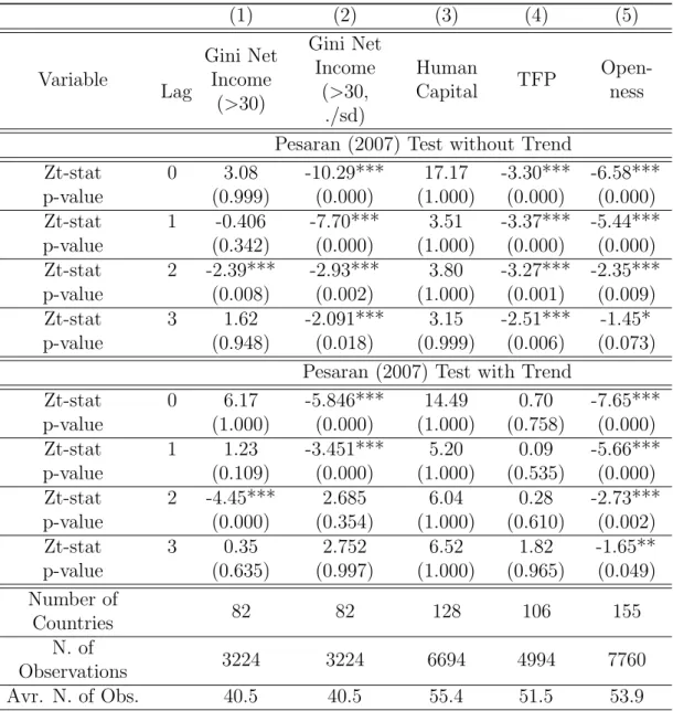
Another issue to be dealt with is the integration level of the series, i.e. its stationarity or non-stationarity. It is well-known that most macro time series are non-stationary even though the issue has received virtually no attention in traditional panel regression analyses (Phillips and Moon, 2000: 264). The graphic analysis in Jaumotte, Lall and Papageorgiou (2013: 277-283) is a means for observing non-stationarity of Gini coefficients and their determinants. Table 3 shows unit root tests. We use the Pesaran (2007) Panel Unit Root test whose null is that the variable is I(1). The analysis of results – with the majority of the tests on the level variables not rejecting – points out the non-stationarity of the Gini coefficients and some of their determinants, with particularly clear results for human capital. The only determinant of inequality for which the tests clearly reject non-stationarity is Openness. These results are confirmed by the tests on the differenced variables (see Table A.1), which clearly reject the unit root case.

This section provides clear empirical motivation that the heterogeneous panels unobserved common factors framework from Pesaran (2006) and followers is appropriate to analyze in-equality determinants. The availability of data in quality and quantity allow for its correct implementation.

The next section explores the causal relationship between inequality and human capital.

12_{Variables linked with disposable income have also been the focus of earlier papers. Barro (2000) uses a}

dummy to account for differences from the net income and consumption definition and gross income definition. This dummy is highly significant indicating that these variables measure in fact different phenomena. Jaumotte, Lall and Papageorgiou (2013: 276) also express concern about jointly analyzing income and expenditure-based Gini indexes. Results obtained with the market Gini coefficient (and its uncertainty-corrected version), which can compare with the ones presented in the paper, can be provided by the authors.

1 2 3 4 5 6 7 8 9 10 11 12 13 14 15 16 17 18 19 20 21 22 23 24 25 26 27 28 29 30 31 32 33 34 35 36 37 38 39 40 41 42 43 44 45 46 47 48 49 50 51 52 53 54 55 56

(15)

For Review Only

Table 3: Panel Unit-Root tests

(1) (2) (3) (4) (5) Variable Lag Gini Net Income (>30) Gini Net Income (>30, ./sd) Human Capital TFP Open-ness Pesaran (2007) Test without Trend

Zt-stat 0 3.08 -10.29*** 17.17 -3.30*** -6.58*** p-value (0.999) (0.000) (1.000) (0.000) (0.000) Zt-stat 1 -0.406 -7.70*** 3.51 -3.37*** -5.44*** p-value (0.342) (0.000) (1.000) (0.000) (0.000) Zt-stat 2 -2.39*** -2.93*** 3.80 -3.27*** -2.35*** p-value (0.008) (0.002) (1.000) (0.001) (0.009) Zt-stat 3 1.62 -2.091*** 3.15 -2.51*** -1.45* p-value (0.948) (0.018) (0.999) (0.006) (0.073)

Pesaran (2007) Test with Trend

Zt-stat 0 6.17 -5.846*** 14.49 0.70 -7.65*** p-value (1.000) (0.000) (1.000) (0.758) (0.000) Zt-stat 1 1.23 -3.451*** 5.20 0.09 -5.66*** p-value (0.109) (0.000) (1.000) (0.535) (0.000) Zt-stat 2 -4.45*** 2.685 6.04 0.28 -2.73*** p-value (0.000) (0.354) (1.000) (0.610) (0.002) Zt-stat 3 0.35 2.752 6.52 1.82 -1.65** p-value (0.635) (0.997) (1.000) (0.965) (0.049) Number of Countries 82 82 128 106 155 N. of Observations 3224 3224 6694 4994 7760 Avr. N. of Obs. 40.5 40.5 55.4 51.5 53.9

Note: All variables are in natural logarithms. >30 indicates that only cross-sections with more that 30 time-series observations are included. ./sd indicates when the Gini coefficient is divided by the source standard-deviation to account for data uncertainty. Level of significance: *** for

p-value<0.01; **for p-value<0.05;* for p-value<0.1. 1 2 3 4 5 6 7 8 9 10 11 12 13 14 15 16 17 18 19 20 21 22 23 24 25 26 27 28 29 30 31 32 33 34 35 36 37 38 39 40 41 42 43 44 45 46 47 48 49 50 51 52 53 54 55 56 57

(16)

For Review Only

4.2 Initial Analysis: causality between education and inequality

Trade and productivity (or technology) as determinants of inequality have been widely studied and the causal relationship from openness and technology to inequality is well founded in theory (see e.g. Hornstein, Krusel and Violante, 2005, Chakrabarti, 2000, and Richardson, 1995). However, the causality path from human capital to inequality is not so well founded. Despite the tremendous emphasis on the role of human capital in the skill-biased technological change and general purpose technology literatures, there are some microeconomic arguments that come from the economics of education field suggesting that inequality may decrease incentives to educate and thus decrease human capital (Stock´e et al, 2011 and Gutierres and Tanaka, 2009 are good examples that emphasize the causality channel from inequality to education). It is important then to evaluate evidence in our data from the causality channel between human capital and inequality. We do this using a cointegration test for the null of no cointegration, the Westerlund (2007) test.13 _{Table 4 presents the tests when the causality is evaluated between}

human capital and the uncertainty-corrected Gini coefficient. The intuition is as follows. If the null is rejected for a test in which the dependent variable is inequality and simultaneously the null is not rejected for a test in which the dependent variable is human capital, then human capital has a (Granger-) causal effect on inequality and inequality has no (Granger-) causal effect on human capital. The pattern of results clearly suggests a (Granger-) causal relationship from human capital to inequality and not the other way around, tending to validate an empirical strategy that estimates the relationship theoretically implied by the skill-biased technological change framework. This is valid for both the uncertainty-corrected measure presented in Table 4 and for the uncorrected measure.14 _{As in previous tests, we use only cross-sections that have}

availability of time-series data of 30 or more periods.

The next sections present results for the influence of human capital, TFP, and openness on inequality using heterogeneous panels methods.

13_{An example in the literature that use this test to motivate the underlying channel of causality is in Eberhardt}

and Presbitero (2014).

14_{Results for the uncorrected measure are in Table A.2.}

1 2 3 4 5 6 7 8 9 10 11 12 13 14 15 16 17 18 19 20 21 22 23 24 25 26 27 28 29 30 31 32 33 34 35 36 37 38 39 40 41 42 43 44 45 46 47 48 49 50 51 52 53 54 55 56

(17)

For Review Only

Table 4: Cointegration tests

(1) (5) (6) (7) (8)

Lag Trend Test Gt Test Ga Test Pt Test Pa

Dependent

Variable Gini Coefficient net income (>30, ./sd)

1 No -2.400*** -10.22*** -9.630*** -9.588*** p-value (0.001) (0.004) (0.002) (0.000) 1 Yes -2.653** -12.64 -10.79 -11.343** p-value (0.049) (0.332) (0.156) (0.033) 2 No -2.353*** -8.232 -7.195 -7.261*** p-value (0.001) (0.174) (0.342) (0.000) 2 Yes -2.689** -10.952 -7.660 -8.500 p-value (0.031) (0.768) (0.995) (0.630) Dependent

Variable Human Capital

1 No -1.826 -3.711 -5.713 -1.453 p-value (0.401) (0.998) (0.861) (0.998) 1 Yes -1.990 -7.607 -9.765 -6.089 p-value (0.985) (0.999) (0.565) (0.985) 2 No -1.879 -3.855 -5.448 -1.406 p-value (0.298) (0.998) (0.912) (0.999) 2 Yes -1.807 -7.110 -8.696 -5.479 p-value (0.999) (1.000) (0.917) (0.996)

Note: All variables are in natural logarithms. >30 indicates that only cross-sections with more that 30 time-series observations are included. All tests include a constant. ./sd indicates when the Gini coefficient is divided by the source standard-deviation to account for data uncertainty. Level of

significance: *** for p-value<0.01; **for p-value<0.05;* for p-value<0.1. Rejection of H0 in Ga and Gt tests should be taken as evidence of cointegration of at least one of the cross-sectional units. Rejection of H0 in Pa and Pt tests should therefore be taken as evidence of cointegration for

the panel as a whole. 1 2 3 4 5 6 7 8 9 10 11 12 13 14 15 16 17 18 19 20 21 22 23 24 25 26 27 28 29 30 31 32 33 34 35 36 37 38 39 40 41 42 43 44 45 46 47 48 49 50 51 52 53 54 55 56 57

(18)

For Review Only

4.3 Results: baseline specification

In this section we present the results for our baseline specification in equation (1).

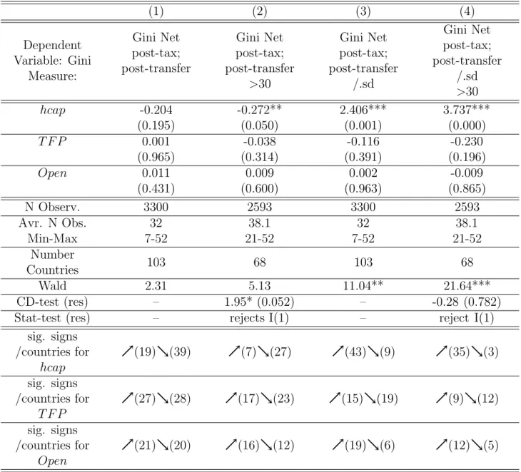
Results in Table 5 show that, for uncorrected Gini indexes, human capital, TFP and Open-ness are not quite significant which may mean that there is great heterogeneity concerning effects of the three determinants across countries. Human capital is significant only in the re-gression for the Gini coefficient - with a negative sign when the Gini coefficient is not corrected for uncertainty and for the restricted sample with longer time-series within panels - Table 5, column (2) and with a positive sign when the Gini coefficient is corrected for uncertainty -Table 5, columns (3) and (4). In the former case, an increase in 1% in human capital would imply a decrease of 0.27% in the uncorrected Gini coefficient. In the later, however, a 1% increase in human capital would increase the corrected Gini coefficient from 2.4% to 3.7%. Alternatively, it can be said that for the same level of precision of the Gini coefficient, a 1% increase in human capital would increase the Gini coefficient in values ranging from 2.4% to 3.7%. The variability of effects across countries can be observed by the count of significant effects by country, provided in the Table. The number of countries with significant results for each variable are usually more than 50% of the number of countries included in the regressions. While the overwhelming number of countries present significant positive coefficients for human capital, the number of significantly positive and negative coefficients for TFP and Openness are relatively balanced, possibly indicating the great variability in the relationship between TFP and Openness and inequality between countries.15

4.4 Results: sub-samples

In order to evaluate the effects of human capital, TFP, and openness in different groups of countries, we now split our sample according to the level of income, inequality, human capital,

15_{We follow Eberhardt and Presbitero (2014) in showing counts of significant effects. However, due to the}

fact that we cannot rely on country-specific estimates of standard-errors, we do not analyse the effects of each country. Alternatively, we construct sub-samples of countries to explore deeply that heterogeneity.

1 2 3 4 5 6 7 8 9 10 11 12 13 14 15 16 17 18 19 20 21 22 23 24 25 26 27 28 29 30 31 32 33 34 35 36 37 38 39 40 41 42 43 44 45 46 47 48 49 50 51 52 53 54 55 56

(19)

For Review Only

Table 5: Inequality, Human Capital, TFP, and Openness

(1) (2) (3) (4) Dependent Variable: Gini Measure: Gini Net post-tax; post-transfer Gini Net post-tax; post-transfer >30 Gini Net post-tax; post-transfer /.sd Gini Net post-tax; post-transfer /.sd >30 hcap -0.204 -0.272** 2.406*** 3.737*** (0.195) (0.050) (0.001) (0.000) T F P 0.001 -0.038 -0.116 -0.230 (0.965) (0.314) (0.391) (0.196) Open 0.011 0.009 0.002 -0.009 (0.431) (0.600) (0.963) (0.865) N Observ. 3300 2593 3300 2593 Avr. N Obs. 32 38.1 32 38.1 Min-Max 7-52 21-52 7-52 21-52 Number Countries 103 68 103 68 Wald 2.31 5.13 11.04** 21.64*** CD-test (res) – 1.95* (0.052) – -0.28 (0.782)

Stat-test (res) – rejects I(1) – reject I(1)

sig. signs /countries for hcap (19)(39) (7)(27) (43)(9) (35)(3) sig. signs /countries for T F P (27)(28) (17)(23) (15)(19) (9)(12) sig. signs /countries for Open (21)(20) (16)(12) (19)(6) (12)(5)

Note: Dependent Variables are natural logarithm of the Gini coefficients. All variables are in natural logarithms. hcap is human capital, TFP is total factor productivity and Open is Openness ratio. Values between parentheses below coefficients are p-values from robust (clustered) standard errors. Level of significance: *** for p-value<0.01; **for p-value<0.05;* for p-value<0.1. Wald test is a joint significance test for the regressors. CD-test is a

Pesaran (2004) cross-section dependence test on the null of cross-section independence done on the residuals from the regression (p-value presented between parentheses). Stat-test is the Pesaran (2007) unit root test made on the residuals. This test used 3 lags and rejects I(1) means that in all

lags the test of unit root rejects. sig. signs/countries for hcap, TFP or Open presents the count of countries with positive or negative statistical significant coefficient. /(sd) indicates when the Gini coefficient is divided by the source standard-deviation to account for data uncertainty. The list

of countries that enter in columns (3) and (4) are provided in the Appendix B. 1 2 3 4 5 6 7 8 9 10 11 12 13 14 15 16 17 18 19 20 21 22 23 24 25 26 27 28 29 30 31 32 33 34 35 36 37 38 39 40 41 42 43 44 45 46 47 48 49 50 51 52 53 54 55 56 57

(20)

For Review Only

TFP and openness. With this, we aim to deeply analyse the heterogeneity in this equilibrium relationship between inequality and its determinants. We used the sample median for real GDP per capita, the (corrected) Gini index, human capital, TFP and openness as the thresholds to split the sample in each case. For example, a country with an average of GDP per capita above the median would be classified as rich country.

Results in Table 6, Table 7 and Table 8 show that the positive effect of human capital on inequality, once it is corrected for uncertainty in data, occurs mainly in rich countries, in countries with high human capital and in countries with high TFP. In these countries a 1% increase in human capital would imply that the corrected Gini coefficient increase from 3.2% to 4.8%. The fact that the positive effect of human capital in inequality is particularly evident on the group of rich countries is consistent with the skill-biased technical change theory, according to which the increase in human capital stocks should be associated with the adoption of skill-biased technologies, which in turn positively influence the wages of the richest in the economy. This effect may overcome the supply effect and is present mostly in the rich countries (see e.g. Hornstein, Krusel and Violante, 2005: 1306). In the high human capital sample and in the low TFP sample, we obtain a negative statistically significant effect of TFP on inequality, which is not confirmed in the other subsamples.

Table 9 shows results for regressions of subsamples of high inequality countries and low inequality countries. The stronger result is confirmed for high inequality countries, but we have also obtained a statistically significant result for low inequality countries (in the restricted sample, column (4)). In this case, a 1% increase in human capital would imply that the corrected Gini coefficient increases 1.2%.

Finally, Table 10 shows results for regressions of subsamples of countries with high open-ness to trade and low openopen-ness to trade. In this case we obtain a slightly higher effect of human capital in inequality in highly opened countries than the obtained for countries with less openness to trade. However, the effect of human capital is highly significant in both groups of countries. While in the group of countries highly opened to trade a 1% increase in human capital would imply that the corrected Gini coefficient increases from 3.3% to 4.8%, in the

1 2 3 4 5 6 7 8 9 10 11 12 13 14 15 16 17 18 19 20 21 22 23 24 25 26 27 28 29 30 31 32 33 34 35 36 37 38 39 40 41 42 43 44 45 46 47 48 49 50 51 52 53 54 55 56

(21)

For Review Only

Table 6: Inequality, Human Capital, TFP, and Openness (Rich versus Poor countries)

Rich Sample Poor Sample

(1) (2) (3) (4) Dependent Variable: Gini Measure Gini Net post-tax; post-transfer (./sd)

Gini Net post-tax; post-transfer (>30, ./sd) Gini Net post-tax; post-transfer (./sd)

Gini Net post-tax; post-transfer (>30, ./sd) hcap 4.043*** 3.157*** 1.169 0.518 (0.002) (0.005) (0.239) (0.487) T F P -0.127 -0.251 -0.041 -0.030 (0.656) (0.444) (0.717) (0.860) Open 0.032 -0.119 0.001 -0.078 (0.784) (0.242) (0.985) (0.315) N Observ. 1657 1431 1643 1162 Avr. N Obs. 36.8 40.9 28.3 35.2 Min-Max 12-52 22-52 7-48 21-48 Number Countries 45 35 58 33 Wald 9.77** 9.98** 1.52 1.52 CD-test (res) – -1.40 (0.162) – -0.79 (0.430) Stat-test

(res) – reject I(1) – reject I(1)

Note: Dependent Variables are natural logarithm of the Gini coefficients. All variables are in natural logarithms. hcap is human capital, TFP is total factor productivity and Open is Openness ratio. A constant is included in all regressions but omitted from the Table. Values between parentheses

below coefficients are p-values from robust (clustered) standard errors. Level of significance: *** for p-value <0.01; **for p-value<0.05;* for p-value<0.1. Wald test is a joint significance test for the regressors. CD-test is a Pesaran (2004) cross-section dependence test on the null of cross-section independence done on the residuals from the regression (p-value presented between parentheses). Stat-test is the Pesaran (2007) unit root test made on the residuals. This test used 3 lags and rejects I(1) means that in all lags the test of unit root rejects. /(sd) indicates when the

Gini coefficient is divided by the source standard-deviation to account for data uncertainty.

group of countries less opened to trade, a 1% increase in human capital would imply that the corrected Gini coefficient increases from 2.2% to 2.7%.

Below, we present a set of robustness analysis to evaluate the effect of human capital and TFP on inequality, using the uncertainty-corrected measure of the Gini coefficient.

4.5 Results: alternative specifications

In the robustness analysis we have implemented slightly modified common correlated effects estimators as suggested in recent literature. We include in regressions one or more further covariates in the form of cross-section averages, which helps to identify the unobserved common

1 2 3 4 5 6 7 8 9 10 11 12 13 14 15 16 17 18 19 20 21 22 23 24 25 26 27 28 29 30 31 32 33 34 35 36 37 38 39 40 41 42 43 44 45 46 47 48 49 50 51 52 53 54 55 56 57

(22)

For Review Only

Table 7: Inequality, Human Capital, TFP, and Openness (High versus Low Inequality)

High Inequality Sample Low Inequality Sample

Gini Net post-tax; post-transfer (>30, ./sd) hcap 3.92*** 4.519*** 0.423 1.16** (1.304) (1.324) (0.680) (0.557) T F P -0.337 -0.172 -0.084 -0.007 (0.309) (0.376) (0.124) (0.167) Open 0.159 0.051 0.013 0.011 (0.107) (0.112) (0.046) (0.053) N Observ. 2017 1659 1283 934 Avr. N Obs. 35.4 40.5 27.9 34.6 Min-Max 9-52 22-52 7-52 21-52 Number Countries 57 41 46 27 Wald 12.43*** 12.07*** 0.92 4.39 CD-test (res) – -2.07** (0.039) – -1.87* (0.061) Stat-test

Gini coefficient is divided by the source standard-deviation to account for data uncertainty. 1 2 3 4 5 6 7 8 9 10 11 12 13 14 15 16 17 18 19 20 21 22 23 24 25 26 27 28 29 30 31 32 33 34 35 36 37 38 39 40 41 42 43 44 45 46 47 48 49 50 51 52 53 54 55 56

(23)

For Review Only

Table 8: Inequality, Human Capital, TFP, and Openness (High versus Low Human Capital Index)

High Human Capital Sample Low Human Capital Sample

Gini Net post-tax; post-transfer (>30, ./sd) hcap 3.92** 4.23*** 0.843 2.562 (1.572) (1.341) (1.200) (1.730) T F P -0.271 -0.424** -0.081 -0.224 (0.225) (0.209) (0.156) (0.308) Open 0.153* 0.112 -0.033 -0.013 (0.088) (0.089) (0.043) (0.101) N Observ. 2162 1849 1138 744 Avr. N Obs. 34.3 38.5 28.4 37.2 Min-Max 9-52 21-52 7-48 31-48 Number Countries 63 48 40 20 Wald 10.69** 15.64*** 1.35 2.74 CD-test (res) – -1.76* (0.078) – -0.22 (0.825) Stat-test

Gini coefficient is divided by the source standard-deviation to account for data uncertainty. 1 2 3 4 5 6 7 8 9 10 11 12 13 14 15 16 17 18 19 20 21 22 23 24 25 26 27 28 29 30 31 32 33 34 35 36 37 38 39 40 41 42 43 44 45 46 47 48 49 50 51 52 53 54 55 56 57

(24)

For Review Only

Table 9: Inequality, Human Capital, TFP, and Openness (High versus Low TFP)

High TFP Sample Low TFP Sample

Gini Net post-tax; post-transfer (>30, ./sd) hcap 4.851*** 4.687*** -0.564 0.974 (0.981) (0.974) (1.317) (1.374) T F P -0.164 -0.042 0.018 -0.264* (0.173) (0.220) (0.127) (0.142) Open -0.081 -0.118 -0.008 -0.135 (0.097) (0.081) (0.055) (0.094) N Observ. 1629 1463 1671 1130 Avr. N Obs. 38.8 41.8 27.4 34.2 Min-Max 8-52 31-52 7-51 21-51 Number Countries 42 35 61 33 Wald 26.05*** 25.28*** 0.22 6.03 CD-test (res) – -1.04 (0.298) – -1.24 (0.214) Stat-test

Gini coefficient is divided by the source standard-deviation to account for data uncertainty. 1 2 3 4 5 6 7 8 9 10 11 12 13 14 15 16 17 18 19 20 21 22 23 24 25 26 27 28 29 30 31 32 33 34 35 36 37 38 39 40 41 42 43 44 45 46 47 48 49 50 51 52 53 54 55 56

(25)

For Review Only

Table 10: Inequality, Human Capital, TFP, and Openness (High versus Low Openness)

High Openness Sample Low Openness Sample

Gini Net post-tax; post-transfer (>30, ./sd) hcap 3.34** 4.814*** 2.174** 2.71** (1.330) (1.413) (1.055) (1.374) T F P -0.098 -0.010 -0.042 -0.074 (0.227) (0.233) (0.160) (0.252) Open -0.006 -0.027 0.028 -0.069 (0.076) (0.083) (0.052) (0.073) N Observ. 1677 1296 1623 1297 Avr. N Obs. 32.9 39.3 31.2 37.1 Min-Max 12-52 22-52 7-52 21-52 Number Countries 51 33 52 35 Wald 6.5* 11.71*** 4.61 4.86 CD-test (res) – 0.21 (0.833) – -2.16** (0.031) Stat-test

Gini coefficient is divided by the source standard-deviation to account for data uncertainty. 1 2 3 4 5 6 7 8 9 10 11 12 13 14 15 16 17 18 19 20 21 22 23 24 25 26 27 28 29 30 31 32 33 34 35 36 37 38 39 40 41 42 43 44 45 46 47 48 49 50 51 52 53 54 55 56 57

(26)

For Review Only

factors (in the spirit of Pesaran, Smith and Yamagata, 2013). Moreover, we also follow Chudik and Pesaran (2013) in introducing lags of cross-section averages in order to account for possible feedback effect from inequality to human capital.16

To this end, we consider openness as a cross-section average, seeking to identify the unob-served common factors as linked with globalization and global integration (e.g. the entrance of China in global market or international crisis affecting all the countries which can hit coun-tries differently). Column (1) in Table 11 presents these results. In column (2) in the same table we present regressions in which we identify the common unobserved factors as, not only globalization and integration (using the variable openness as cross-section average) but also technological spillovers (using the variable TFP as cross-section average). In column (3) we add to the set of possible unobserved common factors, production spillovers, including GDP per capita as a cross-section average. In column (4) we consider only openness as cross-section average and eliminate TFP from the regression. This regression aims to show that the ro-bustness of the positive effect of human capital on inequality is not dependent on the presence of TFP, and thus, not dependent on the way this particular TFP measure is calculated. In columns (5) and (6) we also include lags of the cross-section averages.17

In this robustness analysis we consider as dependent variable the Gini coefficient (net defi-nition), using only cross-sections with more than (or equal to) 30 time-series observations. This is done to allow for diagnostic testing. We will also describe the results obtained with the same variable from all the cross-sections (independently of time-series coverage).

In regressions in which production spillovers are not considered as cross-country common factor - columns (1), (2) and (4) - the effect of human capital is highly significant meaning that a 1% increase in human capital would imply a rise in the level of inequality that is around 3.8%. From these, columns (1) and (2) present residuals that show no evidence of nonstationarity or cross-country dependence. Regression residuals from column (4) regression present some

16_{This is similar to what Eberhardt and Presbitero (2014) did in an empirical implementation for the}

rela-tionship between growth and debt.

17_{We closely follow the rule of thumb suggested by Chudik and Pesaran (2013) - p = T}1/3 _{- and include 3 to}

4 lags of the cross-section averages.

1 2 3 4 5 6 7 8 9 10 11 12 13 14 15 16 17 18 19 20 21 22 23 24 25 26 27 28 29 30 31 32 33 34 35 36 37 38 39 40 41 42 43 44 45 46 47 48 49 50 51 52 53 54 55 56

(27)

For Review Only

evidence of cross-country dependence (yet much lower than in the regressors) and no evidence of nonstationarity. In fact, as in Eberhardt and Prebistero (2014), the introduction of additional cross-country averages in regressions helps to obtain cross-country independence of residuals. In the regression that includes production spillovers as a possible common factor - column (3) - the effect of human capital decreases quantitatively but maintains the high level of significance. In this case, a 1% increase in human capital would imply a rise in the level of inequality of around 1.9%. Additionally residuals show no evidence for cross-country dependence or nonstationarity. For regressions robust to potential feedback effect from inequality to human capital - columns (5) and (6) - the effect of human capital is also significantly positive with comparable absolute effects (3.31% and 2.97% respectively) although the statistical significance is decreased from previous regressions. Wald tests point to high significance of the regressors.

Regressions that include all the cross-sections (and not only those with high time-series coverage, as those in the Table 11) would confirm those results. Regressions corresponding to those in columns (1), (2) and (4) slightly decrease the effect of human capital to a coefficient from 2.8 to 3.17 (with a high significance corresponding to p-values of 0.000). Regression corresponding to that in column (3) decreases the quantitative effect and the level of significance (to a value near 0.8 and a significance level of near 0.25). Regressions corresponding to those in columns (5) and (6) highly increase the statistical significance of the human capital coefficient and also its absolute value, with 4.7% increase in inequality deriving from a 1% change in human capital.

4.6 Discussion, Robustness and Policy implications

In this section we critically discuss our results and also present some information about ad-ditional tests that are not presented in the paper but that are available upon request. We present evidence on the effects of human capital, TFP and openness on inequality. To that end, we used a recent measure of inequality with high coverage (Solt, 2009) and also recently developed estimators that allow for country heterogeneity and are robust to country

depen-1 2 3 4 5 6 7 8 9 10 11 12 13 14 15 16 17 18 19 20 21 22 23 24 25 26 27 28 29 30 31 32 33 34 35 36 37 38 39 40 41 42 43 44 45 46 47 48 49 50 51 52 53 54 55 56 57

(28)

For Review Only

Table 11: Inequality, Human Capital, TFP, and Openness (Robustness) Dependent

Variable Gini Coefficient net income (./sd, >30)

Vars. only as

CS Avr. Open Open; TFP

Open; TFP; GDP p.c. Open; without TFP TFP Open; TFP Lags of CS Avr. 0 0 0 0 3 (TFP); 4 (other) 3 (TFP, Open); 4 (other) (1) (2) (3) (4) (5) (6) hcap 3.801*** 3.854*** 1.984*** 3.716*** 3.312** 2.974* (0.000) (0.000) (0.001) (0.000) (0.026) (0.075) T F P -0.204 – – – – – (0.248) N Observ. 2593 2855 2855 2855 2383 2240 Avr. N Obs. 38.1 38.6 38.6 38.6 32.2 33.9 Min-Max 21-52 21-52 21-52 21-52 17-48 24-48 Number Countries 68 74 74 74 74 66 Wald 78.80*** 97.11*** 75.50*** 133.90*** 49.13*** 36.07*** CD-test (res) -0.20 0.81 -1.01 1.89* 1.12 0.52 (0.839) (0.420) (0.314) (0.058) (0.261) (0.602) Stat-test

(res) Reject I(1) Reject I(1) Reject I(1) Reject I(1) Reject I(1) Reject I(1)

sig. signs /countries for hcap (37)(2) (44)(6) (22)(9) (42)(8) (13)(9) (14)(6) sig. signs /countries for T F P (12)(15) – – – – –

Note: Note: Dependent Variables are natural logarithm of the Gini coefficients. All variables are in natural logarithms. hcap is human capital, TFP is total factor productivity and Open is Openness ratio. A constant is included in all regressions but omitted from the Table. Values between parentheses below coefficients are p-values from robust (clustered) standard errors. Level of significance: *** for p-value <0.01; **for p-value<0.05;*

for p-value<0.1. Wald test is a joint significance test for the regressors. CD-test is a Pesaran (2004) cross-section dependence test on the null of cross-section independence done on the residuals from the regression (p-value presented between parentheses). Stat-test is the Pesaran (2007) unit root test made on the residuals. This test used 3 lags and rejects I(1) means that in all lags the test of unit root rejects. sig. signs/countries for hcap,

TFP or Open presents the count of countries with positive or negative statistical significant coefficient. /(sd) indicates when the Gini coefficient is divided by the source standard-deviation to account for data uncertainty. The list of countries that enter in columns (3) and (4) are presented in

Appendix B. 1 2 3 4 5 6 7 8 9 10 11 12 13 14 15 16 17 18 19 20 21 22 23 24 25 26 27 28 29 30 31 32 33 34 35 36 37 38 39 40 41 42 43 44 45 46 47 48 49 50 51 52 53 54 55 56

(29)

For Review Only

dence, stationarity and endogeneity toward unobserved common factors (generally described in the survey from Eberhardt and Teal, 2011). We found a positive robust effect of human capital on inequality and non-significant effects of TFP and Openness. We also discovered that the influence of higher human capital in higher inequality is totally dependent on correcting the Gini coefficient for its measurement uncertainty (with a measure of uncertainty provided by the source). According to Solt (2009) the provided standard-error for the Gini coefficient aims to correct the remaining uncertainty in the estimations for the inequality measure. This standard-error measures the remaining error due to lack or poorer information available for some country-year pairs. Interestingly, ignoring this correction would yield a negative and significant effect of human capital on inequality, thus implying allegedly that human capital investments would decrease inequality. A deep analysis of the data reveals that such a neg-ative sign of the coefficient for the uncorrected Gini index is due to poorer precision in Gini coefficients. For instance, restricting the regression of column (1) in Table 5 to values for the Solt (2009) standard-error above the third quartile (the most unprecise Gini coefficients) would yield a significantly negative coefficient of -0.788 (with a p-value of 0.000) and doing the same to the regression of column (2) in the same Table would yield a coefficient of -0.596 (with a p-value of 0.010). Thus, there is a clear need to account for these differences in quality of the source data when assessing the determinants of inequality.

There are two main issues that might compromise our results: (1) the use of a certain measure of human capital and (2) the correction of the Gini measure with the source standard-error to account for different data quality across the world. Would it be possible that this effect is linked with the specific human capital variable used in this paper? In fact, measurement of human capital has always been somewhat controversial in the literature. The measure of human capital that is most used in the literature is that of Barro and Lee (2001), which has been criticized by e.g. Cohen and Soto (2007) due to measurement errors and sources. In fact, Cohen and Soto (2007) argued to have crucially increased the data quality when compared to their predecessors. Barro and Lee (2013), in the version 1.3 of the database, updated the data to incorporate the criticism. The PWT 8.0 human capital variable used in this paper builds on

1 2 3 4 5 6 7 8 9 10 11 12 13 14 15 16 17 18 19 20 21 22 23 24 25 26 27 28 29 30 31 32 33 34 35 36 37 38 39 40 41 42 43 44 45 46 47 48 49 50 51 52 53 54 55 56 57

(30)

For Review Only

Barro and Lee database, version 1.3. Additionally, the authors of PWT 8.0 filled in the years between the 5 year intervals provided by Barro and Lee, using linear interpolation and corrected the years of schooling to different returns from schooling by level of education following a Mincerian approach. There are, of course, some limitations of this measure, especially the fact that it does not distinguish the returns from schooling by country and by year. An exploration of the returns to schooling variability in a human capital measure would certainly be obtained at the cost of reducing the country coverage and increasing measurement error. Thus, the human capital variable from PWT 8.0 is the human capital data with widest coverage, and thus the only that consistently allow for the use of heterogeneous panel data methods. In order to investigate if the use of returns to obtain the Mincerian-consistent measure of the PWT 8.0, we repeated the regressions in Tables 5, 6 to 11 using two original alternative variables from Barro and Lee (2013), educational attainment above 15 and 25 years (which were linearly interpolated to obtain comparable series to the one used in the benchmark analysis). The results showed very consistently with previous ones, showing a highly statistical significant and positive effect of human capital on inequality for both variables in all specifications. When comparing the obtained results with those of the tables above, we noted that despite the very high statistical significance (almost always with p-values equal to 0.000), coefficients are slightly lower than those presented on the tables, oscillating between 1.3 and 2.6, indicating that a 1% increase in years of schooling imply an increase in inequality from 1.3% to 2.6%. The remaining effect to those reported in the tables above should be attributed to differences in returns throughout the different levels of schooling. In order to investigate whether the interpolation approach would have eliminated the significance of our results, we ran regressions that eliminated the interpolated observations. This greatly decreased the number of observations available for each regression from nearly 3200 observations to nearly 500 observations. Nevertheless, all regressions corresponding to specifications presented earlier in Table 1118 _{maintain the highly}

significant positive signed human capital coefficient, with statistical significance of 5% or less.

18_{Considering specifications in columns (1) to (4), as the time-series requirements of specifications in columns}

(5) and (6) are not met when considering only five-year periods.

1 2 3 4 5 6 7 8 9 10 11 12 13 14 15 16 17 18 19 20 21 22 23 24 25 26 27 28 29 30 31 32 33 34 35 36 37 38 39 40 41 42 43 44 45 46 47 48 49 50 51 52 53 54 55 56

(31)

For Review Only

The human capital variable construction and the very robust results we have obtained give us confidence that the obtained results must be common to any correct measure of human capital given that it has the wide time-series and cross-country coverage as does this one. As a consequence our strong effect of human capital on inequality has non-negligible policy effects. Until now, and given the results in Barro (2000), the common wisdom has been that if some education increases inequality, it should be the higher levels of education. However, by con-struction, the employed measure of human capital strongly weights lower levels of education (due to higher returns for lower levels of education). Thus, the effect of education on inequality is particularly due to lower levels of education. This has policy relevance as politicians should be aware of this effect in promoting education, even at the lower levels. Notwithstanding, this effect is absent from the poorer countries, which indicates no influence of education in increas-ing inequality on those countries. Thus, generally, in poorer countries, policy may enhance education with no caution about rising inequality. On the contrary, on the rich countries, improvements in education may call for redistributive fiscal policy.

The second issue is related to the correction of the Gini coefficient. We did that by simply dividing the Gini coefficient by the standard-error, as explained above. This standard-error oscillates in the sample from 0.0016 to 15.43, which gives an idea of the difference in quality remaining in data and suggests the need to account for these quality heterogeneity. In fact, 25% of the observations present a standard-error below 0.5. Dividing the Gini coefficient by this standard-error would greatly magnify Gini coefficients in the case of high precision (i.e. when standard-deviations approach zero). A correction that would not present that property would be the division of the Gini coefficient by (1+standard-error).19 _{With this, a high}

precision Gini coefficient - with a standard-error close to 0 - would not be increased although a low precision coefficient would be decreased. The high significance of human capital positive coefficients hardly changes with this modification in the corrected Gini index in all the different specifications we present in the paper (corresponding to specifications in Tables 5 - columns

19_{The alternative proposed uncertainty-corrected measure is thus} GIN I

1+sd(GIN I), where GINI is the Gini index

provided by SWIID and sd(GINI) is the standard-deviation of the Gini index, also provided by the SWIID and that corrects for uncertainty or measurement error within the sources. Results are provided in Appendix C.

1 2 3 4 5 6 7 8 9 10 11 12 13 14 15 16 17 18 19 20 21 22 23 24 25 26 27 28 29 30 31 32 33 34 35 36 37 38 39 40 41 42 43 44 45 46 47 48 49 50 51 52 53 54 55 56 57