Dissertation
Master in Corporate Finance
The Housing Market in the District of Leiria:
A Hedonic Approach
Cláudia Patricia Ferreira Sousa Carreira
Master Dissertation performed under the supervision of Doctor Natália Maria Prudêncio Rafael Canadas, Professor in the School of Technology and Management of the Polytechnic
Institute of Leiria and co-supervision of Master Maria João Silva Jorge, lecturer in the School of Technology and Management of the Polytechnic Institute of Leiria.
i ACKNOWLEDGEMENTS
This dissertation is the result of much devotion and work hours, sometimes accompanied by many uncertainties and doubts. However, my willpower and persistence overcame all obstacles and, as a result, I managed to finish this work with satisfaction and enthusiasm.
My dissertation is the corollary of two years of effort and dedication. The frequency of the Master in Corporate Finance allowed me to obtain new knowledge, as well as recycling and learning new methods of research and study. The Master in Corporate Finance undoubtedly contributed to my personal and professional enrichment.
Thus, it is very important for me to kindly thank to all those who contributed and who helped me so that I could carry out this work.
Firstly, I would like to thank my supervisor, Professor Doctor Natália Canadas, for her unconditional support, and also thank my co-supervisor, Master Maria João Jorge, for her time, dedication, availability and suggestions that were crucial to the development of this dissertation.
Then, I would also like to thank Dr. Vanessa Santos from Casa Sapo, for her availability, which was central to the sampling.
Thanks also to my friends, Bárbara Melo and Luísa Morgadinho, for their patience and friendship.
I am also grateful to my dear parents, who supported me unconditionally and always showed patience and understanding. To them I must, in part, the realization of this dream because their help was very important during the past two years. To my husband, Nelson, and my daughters, Maria and Camila, who sometimes were harmed by my absence, and have always known to tolerate my mood changes in my darkest hours.
With all my heart, my thanks to all those who contributed to making this dream come true.
ii ABSTRACT
The real estate housing valuation is, even today, highly subjective. The sales comparison approach, which is based on the determination of housing value suported on sales price of similar housing in a particular market area, remains the most widely used method. Given this situation, the hedonic model should be seen as a solution to improve the quality of assessments, as it determines the price of housing according to the observable values of their different atributes.
This dissertation aims to develop a hedonic model for the housing market in the district of Leiria reported to 2010, in order to verify the characteristics of a house that most influence its price. It is proposed a hedonic model of house prices according to the characteristics of a housing listed by Angli and Gencay (1996), Goodman and Thibodaeu (1997), Maurer, Pitzer and Sebastian (2004), Morancho (2003), Ozzane and Malpezzi (1985), Pozo (2009), Rodrigues (2008), Selim (2008) and Wen, Jia and Guo (2005). The cubic functional form is used to proceed with the empirical study.
The results indicate that the price of a house is strongly influenced by some location variables, neighbourhood variables and structural variables. Some of these variables have a positive effect on the housing price, such as the location of housing in the county of Óbidos and the number of bedrooms of the housing, specifically housing with four or five bedrooms. Other variables have a negative effect on price, such as usage status of a house, namely used housing and the location of housing in the counties of Marinha Grande and Leiria.
Key words: hedonic model, housing market, real estate.
iii TABLE OF CONTENTS
ACKNOWLEDGEMENTS ... i
ABSTRACT ... ii
TABLE OF CONTENTS ... iii
LIST OF TABLES ... v
LIST OF FIGURES ... vi
1.INTRODUCTION ... 1
2.LITERATURE REVIEW ... 2
2.1. Characterization of the housing market and its efficiency ... 2
2.2. State of the art: review of various methods of real estate housing valuation... 3
2.2.1. Traditional valuation methods ... 3
2.2.2. Advanced valuation methods ... 5
2.2.2.1. Artificial neural network... 5
2.2.2.2. Spatial analysis method ... 6
2.2.2.3. Fuzzy logic ... 6
2.2.2.4. Autoregressive integrated moving average (ARIMA) ... 8
2.2.2.5. Hedonic pricing model ... 8
2.3. Brief historical review of hedonic price model ... 8
3.METHODOLOGY... 19
3.1. Problems associated with the hedonic price model ... 19
3.2. Functional form ... 20
3.3. Empirical model specification ... 21
3.4. Source of sample collection ... 22
3.5. Variables definition ... 23
3.5.1 Dependent variable... 23
3.5.2. Independent variables ... 23
4.PRESENTATION AND DISCUSSION OF RESULTS ... 26
4.1. Descriptive statistics ... 26
4.2. Multiple linear regression model ... 27
4.2.1. Selection of the best functional form for the regression model ... 28
4.2.2. Construction of the regression model ... 30
4.2.3. Construction of the regression model without outliers ... 35
iv
5.CONCLUSION ... 44 6.REFERENCES ... 46 Appendix A: Outliers’ analysis ... 51
v LIST OF TABLES
Table 1: Summary of empirical evidence of studies employing the hedonic model... 12
Table 2: Definitions and sources of independent variables... 23
Table 3: Summary statistics of dependent variable and continous independent variables 26 Table 4: Summary statistics of dummy independent variables... 26
Table 5: Determination coefficients and functional forms... 29
Table 6: Coefficients for the variables in the baseline model and significance level... 30
Table 7: Coefficients for the variables in the model and significance level... 33
Table 8: Coefficients for the variables in the final model and significance level... 35
Table 9: Summary of empirical results... 37
Table 10: Kolmogorov-Smirnov test... 41
Table 11: Tolerance and VIF test... 43
vi LIST OF FIGURES
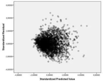
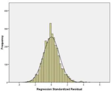
Figure 1: Distribution of observations by counties ... 22 Figure 2: Relationship between standardized residuals and standardized estimated values of the dependent variable ... 39 Figure 3: Relationship between studentized residuals and standardized estimated values of the dependent variable ... 40 Figure 4: Distribution of relative frequencies of residuals and the normal distribution curve ... 41 Figure 5: QQ graphs ... 42
1
1. INTRODUCTION
The housing market has a unique importance because the purchase of a home allows independence and privacy to a person so as to obtain a status in society. Moreover, this market is one of the great engines of a country’s economy. In Portugal, most people have as a priority to buy a house. In fact, this is associated with a sign of “growth in life” and, thus, from the point of view of investment, housing is an asset to which most families channel their economies.
However, due to the crisis that has been experienced in recent times, an adequate estimate of the value of housing is crucial. This forecast will influence the allocation of housing credit which, in turn, will influence the purchase of housing. Moreover, housing has, as main characteristics, durability and spatial fixity, which means that, when a purchase takes effect, there ought to be some reflection.
Despite its importance, the real estate housing valuation is, even today, highly subjective. The most widely used criterion is the one of comparing sales prices in the market, ie, determining the value of housing based on sales’ price of similar housing in a particular market area. Given this situation, the hedonic model should be seen as a solution to improve the quality of assessments, since it allows determining the price of goods according to their attributes. This model allows reducing the degree of subjectivity in the assessment of the value of houses, based on the size, age, architecture, number of the rooms and geographical location, among others.
Aware of the importance of this topic, we intended to develop the issue through an empirical research conducted for the housing market in the district of Leiria reported to 2010. The main objective is the specification of a hedonic model of housing prices. This study consists of four sections. The first section promotes a theoretical framework of the research problem. Specifically, it contains a brief characterization of the housing market, the review of various methods of housing valuation and a brief historical overview of the topic "hedonic price model." In the second section, we present the methodology and the data source. The third section describes and discusses the results. Finally, a fourth section describes the conclusions of the study and highlights also its limitations.
2
2. LITERATURE REVIEW
This section promotes a theoretical framework of the research problem. Specifically, it contains a brief characterization of the housing market, the review of various methods of housing valuation and a brief historical overview of the topic "hedonic price model”.
2.1. Characterization of the housing market and its efficiency
Housing stands out from other goods because it has a set of characteristics that makes it unique.
Durability
One of the most relevant is the durability of housing. Its high duration is a general characteristic. As a result, there is a reduced rate of substitution of such goods.
Spatial fixity
Also important, is the spatial fixity, i.e., such type of good is fixed at a specific location. This is one of the characteristics that will greatly influence the value of the housing. So, there will be a set of exogenous factors to the good that will significantly influence its value. Examples of these factors are:
access to infrastructure;
access to shopping;
transport routes;
quality of neighbourhood;
the jurisdiction of local government.
Heterogeneity
Real estate has, by nature, heterogeneous goods. There are not two equal housing, i.e., there is always some differentiating factor.
Other characteristics
Housing is also distinguished from other assets since the information and transaction costs are high, the liquidity is low, there is a high price for each item and this sector experiences big government intervention.
3
Fama (1970) identified three conditions that are sufficient to make an efficient market: absence of transaction costs, availability of information free of charge and existence of homogeneous expectations among consumers. Based on all the characteristics mentioned above, it may, then, be concluded that there is a low degree of efficiency in housing markets.
2.2. State of the art: review of various methods of real estate housing valuation Pagourtzi, Assimakopoulos, Hatzichristos and French (2003) argue that each country has a different culture and experience that will influence and determine the methods adopted for any particular valuation. The authors divide the methods of housing valuation in two large groups. On the one hand, the traditional methods, which are based on direct observation.These methods are grounded on the direct comparison or may be related with the collection of informations that allows the establishment of a regression model to determine their market value. On the other hand, the advanced methods, which are more quantitative and try to, indirectly, simulate the behaviour of players, in order to estimate the transaction price.
2.2.1. Traditional valuation methods
Next, we present each of the traditional methods: A) Comparable method
To Pagourtzi et al. (2003), the comparable method is the most widely used approach. The housing value is determined based on the sales price of similar housing in a given market area. To apply this method, there is a need to sometimes make adjustments in order to have comparable housing. If two housing are not identical, i.e., there are differences in size, age, construction quality, there must be an adjustment in the selling price to make them comparable. The authors speak of homogenization, i.e., set to be comparable. Thus, they advocate the need to perform the assessment in stages, when using the comparable method. Comparable sales analysis procedure may be viewed as a four-part process: (1) analysis of information on recent transactions of real estate, similar and comparable; (2) adjustment of the selling price, considering the different characteristics of each housing; (3) estimation of the market value and; (4) presentation of results in an accessible and visible set-up.
4
B) Income method
In the income method, the valuation of housing is identified with their ability to generate income. Pagourtzi et al. (2003) argue that income represents the return of money invested in the property by its owner.
C) Profits method
According Pagourtzi et al. (2003), the profits method is based on the analysis of potential income that the housing may generate, less the costs to be incurred to make the house operational to generate such income, here referred to as rent.
D) Residual method
The objective of residual method is to evaluate a vacant land or buildings that should be demolished. The evaluator will study its potential value, providing the revenue owners can get from the land for the development of a new venture. The residual value of land is calculated as the difference between the market value of the project ended and the alleged sum of all costs incurred during the development of the whole process. In short, the residual value of the land represents the maximum amount that an investor will be willing to give the land, so that, after all expenses incurred, he can still get the margin stipulated at the outset.
E) Cost method
The housing valuation by the cost method assumes the value of the reconstruction of a new building, with the same characteristics as the existing structure.
F) Multiple regression method
As its name implies, with the multiple regression method, the housing valuation is made by taking into account the analysis of a set of characteristics that influence the value of the housing. It means that the value of the housing is a variable that depends on a number of other explanatory variables, for example the characteristics of the housing.
G) Stepwise regression method
In the stepwise regression method, evaluation is performed also by a regression. It differs from the previous method since it interactively builds a sequence of regression models by adding or removing variables at each step.
5 2.2.2. Advanced valuation methods
2.2.2.1. Artificial neural network
According to Pagourtzi et al. (2003), an artificial neural network model must first be “trained” from a data set. Afterwards, the model is used to estimate the prices of new homes in the same market. Neural networks are artificial intelligence models originally designed to replicate the human brain’s learning processes.
Limsombunchai, Gan and Lee (2004) argue that neural network consists of three main layers: input data layer (housing attributes), hidden layer(s) (commonly referred to as “black box”), and output layer (estimated house price). In the artificial neural network model, for a particular input, an output is produced. Subsequently, the model compares the output model (estimated house price) to the actual output (actual house price). The accuracy of this value is determined by the total mean square error and then black propagation is used in an attempt to reduce prediction errors, which is done through the adjusting of the connection weights.
Collins and Evans (1994), in their study of housing values with an artificial neural network model, argue that are two phases in the application of the model to a problem: training and interrogation. In the training phase, sets of data are put into the networks, and processed as they pass forward through the layers to the output neurons. For each data set presented to the network, the output neurons give a set of values which at first almost certainly differ greatly from the correct result. The training process is repeated many thousands of times on the same data sets until the network has learnt the underlying pattern in the data. Then, a train network may be interrogated by test data sets. Particularly, as a method of real estate housing valuation, the artificial neural network employs a number of inputs which are physical housing attributes variables, neighbourhood variables and has one output neuron, the value of housing. When learning has been achieved, the network is tested on data which had not been included in the training data set (the control sample). The test results provided by the network are compared with the true selling values of housing in the control sample.
For Nguyen and Cripps (2001), the use of a feed forward artificial neural network with propagation learning presents methodological problems, such as number of hidden layers, number of neurons in each hidden layer, selection and size of training set, selection and
6
size of validation set and overtraining must be addressed. The authors refer that the level of training and the number of hidden neurons affect the memorization and generalized predictability of the model. The model is able to produce the correct results for the training set when the more extensive training and the more hidden neurons are used.
2.2.2.2. Spatial analysis method
According to Pagourtzi et al. (2003), one of the characteristics of the spatial analysis method is that it is able to detect, for example, additional neighbourhood factors that should be considered in explaining variability in the market.
Anselim (1998) argues that the spatial econometrics and spatial statistics are very important for empirical analysis of housing markets. The importance of the spatial aspects of housing markets is unquestioned. For Anselim (1998), the spatial regression approach consists of four main phases: model specification, estimation, diagnosis and model prediction. Typically, a model is first estimated without incorporating spatial effects. The result is the starting point for the diagnosis for spatial effects. On the other hand, the results of spatial regression analysis may also be usefully applied to create “predicted” values at locations or for area units for which no observations are available.
Can and Megbolugbe (1997) also made his contribution for the spatial analysis method, providing a spatial analytical framework for the use of the Geographic Information Systems (GIS) technology in housing market research. It discusses the nature of neighbourhood effects and their influence in housing market. The authors conclude that GIS, coupled with spatial analytical tools, offers an ideal environment for modelling housing data sets.
2.2.2.3. Fuzzy logic
The main characteristic of the fuzzy logic model is to treat or handle the data or information, especially the ambiguous, dubious or even inaccurate one, in innovative ways. A major objective of this method is to translate verbal expressions, often very vague and with a qualitative connotation, into numeric values. The association is made between the verbal expressions with numerical values ranging from 0, when the association is absent, to 1, when the association is total. Another critical aspect of this
7
method is the definition of rules. These rules are based on logical expressions of a kind "if," "or" and "then" with implications of the types:
- If… <condition> then ... ... <result>.
- If ... <condition1> ... and ... <condition2> ... then ... <result>. - If ... <condition1> ... or ... <condition2> ... then ... <result>.
Bagnoli and Smith (1998) demonstrated the application of fuzzy logic to housing market valuation. Fuzzy logic enables a rigorous processing of vague judgments and allows the formalization of the rules from which the judgments are derived. The method also allows their incorporation into formal investment and valuation methods. Bagnoli and Smith (1998), in order to demonstrate how fuzzy logic permits the formalization of the rules from which the judgments are derived, chose the attribute location and, for example, argued that we can interpret the fuzzy rating number as a result of fuzzy rules of the type: if distance is “Near” then the rating number is “Low”. Bagnoli and Smith (1998) believe that the estimated value of housing produced by a fuzzy system should be more realistic than the estimated value produced by a linear regression.
Perng, Hsueh and Yan (2005) analyzed a fuzzy logic decision system for sales-ratio evaluation. The authors argue that the fuzzy logic system consists of four components: fuzzifier, inference engine, rule base and defuzzifier. The process begins with the fuzzification of the key attributes, where the attributes are converted into fuzzy sets. Each fuzzy set consists of linguistic terms and associated memberships. Then the linguistic terms are matched with preconditions of fuzzy if-then rules. The last phase is the defuzzification of consequence terms.
Guan, Zurada and Levitan (2008) argue that, more recently, fuzzy logic has been proposed as non-conventional approach to house price valuation. The authors stated that, in simple cases, one can build membership functions and fuzzy rules using common sense. In the more complex cases, choosing the parameters for a membership is a trial and error process at best. A solution to this problem is to combine the advantages of a fuzzy system with the learning capability of artificial neural networks. The result is an adaptive neuro-fuzzy inference system that allows creation and refinement of fuzzy rules through neural networks.
8
2.2.2.4. Autoregressive integrated moving average (ARIMA)
Pagourtzi et al. (2003), note that ARIMA is the only assessment method that relies on time variables. The ARIMA model is essentially an approach to economic forecasting, based on data time series.
Tse (1997) argues that ARIMA produces forecasts that are likely to be more accurate than the forecasts produced by other approaches. Because short-term factors are expected to change slowly, ARIMA proved to be an excellent short-term model for a wide variety of times series. Tse (1997) asserted that, when a price series crosses its correct moving average, the price series will continue in the direction of the crossing. Briefly, for Tse (1997), the core of the ARIMA model is premised on the fact that the market price is revealed by the pattern of prior price movements.
Chen, Kawaguchi and Patel (2004) argue that ARIMA models suggest many cycles’ in house prices series for many years and these cycles may all be affected by a general business cycle. The authors also argue that a short one-year cycle is also found in all these series and all these cycles have a stochastic nature, suggesting the markets are not steady and are still changing.
2.2.2.5. Hedonic pricing model
Pagourtzi et al. (2003) describe the hedonic pricing model as an advanced method. It will be developed in later sections.
2.3. Brief historical review of hedonic price model
In 1939, Court, an experienced analyst in the American automobile industry, has established the first hedonic price model (Goodman, 1978). The analyst retained the term “hedonic” establishing the price of the car as a function of its different characteristics, which are by nature very heterogeneous.
Later, Lancaster (1966) addressed what was called the “new consumer theory”. This one is distinguished from previous approaches because the goods are not the direct subject of utility, but the utility is derived from their properties or characteristics. The author argues that consumption is an activity in which the goods, either individually or combined, are the inputs and in which the outputs are a collection of their characteristics. The new
9
theory represents a break with the traditional theory since: (1) the good itself does not supply utility or benefit to the consumer; in fact, what provides usefulness are its characteristics; (2) a good has more than one characteristic and some of these characteristics can be shared by more than one good; and (3) a good, when combined with another, has characteristics that are different from the ones it would have if it were considered separately.
To formalize his assumptions, Lancaster (1966) considered the following ones: (1) an individual good or a set of goods is seen as a consumer activity associated with a scale that is not more than the level of activity; (2) each consumption activity produces a vector of fixed characteristics, being its relationship linear; and, (3) one seeks to maximize the utility function of the characteristics of the good.
The model could be analyzed according to the model of Samuelson and Nordhaus (1993), in which the situation of consumption that maximizes its utility is considered taking into account specific budget constraints. In traditional theory, the budget constraint and utility function are related even in the graph of indifference curves. As Lancaster (1966) claims, the utility function can be related with the budget constraint only if they are defined after the same space. There are, then, two choices: to transform the utility function in “goods-space” and relate them directly to the budget constraint, or to change the budget constraint on “characteristics-space” and relate them to the utility function.
Another major driving force advancing towards the consolidation of the hedonic price theory was the work of Rosen (1974). To this researcher, the set called hedonic or implicit prices takes form with the observation of prices of goods and analysis of the characteristics associated with each good. For Rosen (1974), hedonic prices can be defined as the implicit prices of the attributes of different goods and the specific characteristics of each of these goods. The study by Rosen (1974) differs from the one from Lancaster (1966), since it examines not only consumer behaviour but also the market equilibrium. The producers and retailers tend to meet consumer demand at least cost, and buyers (consumers) value the utility of goods.
King (1977) stated that individuals do not buy a good as a good, but as a package of characteristics. It is the characteristics that are valued and the purchase decision depends
10
on the efficiency of each one of them. King (1977), using the hedonic price, estimated the price of a housing based on four characteristics. These are the so-called structural characteristics (Struck); quality interior and exterior (IS); interior space (SPACE); and the land, public services and quality of neighbourhood (SITE). Each characteristic has an associated set of components and each component is part of one and only one characteristic. The value of each characteristic is the sum of the hedonic prices of each of its components. Specifically, the researcher estimated the hedonic price equation based on 683 properties sold in New Haven, in the metropolitan area, between 1967 and 1970. The results were consistent with the “new consumer theory of Lancaster.”
Goodman (1978) also made his contribution to the development of hedonic models in the real estate appraisal, specifically by the sub-division of the market into submarkets. For each submarket, the researcher determined the changes in housing values through a set of components, which are ranked as the structural and neighbourhood. The author applied a hedonic model in his study on properties sold in New Haven between 1967 and 1969. Thus, he divided the market into submarkets, from the centre of New Haven to its suburbs. For each sub-area, he estimated a linear regression based on hedonic prices, and then analysed the differences between the submarkets. In each regression, the value of the housing could be measured based on two types of components: structural and neighbourhood.
Malpezzi (2002), in a selective review of hedonic pricing models, argues that the method of hedonic equations is the decomposition of housing value in measurable quantities and prices. The value of identical or different properties in different places can be predicted and compared. Simply put, a hedonic equation is a regression of the value of housing based on its characteristics. As Malpezzi (2002) discusses, the hedonic model arises because of heterogeneous housing stock and heterogeneous consumers. Not only does each house contain different characteristics, but those characteristics may be valued differently by different consumers.
The author broke down the hedonic equation in the following way:
11
Where:
R = value of housing S = structural characteristics N = neighbourhood characteristics L = location in the market
C = contract conditions
T = time that is given to sale or rent
The author also asserts that the hedonic price model arises due to the heterogeneity of the housing market. He also refers to the hedonic models as two phases models. In the first phase, we have a simple equation which estimates the hedonic price in a superficial way; it simply estimates the effect of characteristics on the value, and only in the second phase we take into account the structural parameters of each individual characteristic.
Malpezzi (2002), in his literature review, argues that:
The distinction between demand and supply, as well as their interaction, has been a “torment” for econometrics.
With the hedonic nonlinear models (logarithmic or other), prices and quantities are correlated. Thus, when consumers choose a quantity of some characteristics, they are implicitly choosing its price.
Another point made by the author is that the costs in the housing market are vast and that adjustments have to be made, assuming that the market is in equilibrium, which, in fact, is not the case. One possible approach to the problem of the imbalance is to estimate hedonic price functions using observations at, or near, equilibrium. We must, then, specify the nature of the process that distinguishes equilibrium from disequilibrium observations, which is not always obvious.
Ottensmann, Payton and Man (2005) also give their contribution to improving the theory of hedonic model of prices in the housing market. The hedonic model used by the authors includes structural characteristics, such as the number of bedrooms, area and the presence of other amenities and it also includes neighbourhood characteristics, such as the quality of schools, the percentage of population of a certain race, the distance to the city centre, among others. The main objective of the authors’ work is to test the performance of
12
alternative measures of location. To test this performance, they retain distance and time to the urban centre, the various centres of employment and measures of accessibility to employment. The authors conclude that the location with respect to employment should be included for the proper specification of hedonic housing price models. The combination of accessibility to employment and change in accessibility to employment provides the best specification of location.
In recent decades, based on housing as a bundle of characteristics, many authors have addressed this issue by giving their contribution to the implementation of the hedonic model in the housing market.
Table 1:
Summary of empirical evidence of studies employing the hedonic model
The table lists the theoretical predictions of influence of the house characteristics on the house price and corresponding empirical evidence. Those studies which provide significant evidence of the theoretical prediction appear after the word “Yes”. Those which findings provide significant evidence but are contrary to the theoretical prediction appear after the word “No”. Those studies that do not support the theoretical prediction appear after the word “No evidence”.
Theorical prediction Empirical Evidence
HOUSE PRICE: Structural Characteristics
House size
Increases when house size increases Yes: Angli and Gencay (1996), Bartik (1987), Bourassa and Peng (1999), Can and Megbolugbe (1997), Canavarro, Caridad and Ceular (2010), Furtado (2007), Goodman and Thibodeau (1995), Goodman and Thibodeau (1997), Morancho (2003), Palmiquist (1984), Pasha and Butt (1996), Parsons (1986), Pozo (2009), Rasmussen and Zuehlke (1990), Rodrigues (2008), Selim (2008), Tse (2002), Wen et al. (2005)
No evidence: Limsombunchai et al. (2004), Neto (2008) Number of bathrooms
Increases when the number of bathrooms increases
No: Angli and Gencay (1996)
Yes: Canavarro et al. (2010), Dubin (1998), Goodman and Thibodeau (1997), King (1977), Limsombunchai et al. (2004), Maurer et al. (2004), Morancho (2003), Ottensmann et
al. (2008), Ozanne and Malpezzi (1985), Palmiquist (1984),
Pasha and Butt (1996), Pozo (2009), Rodrigues (2008)
No evidence: Kain and Quigley (1970), Tarré (2009), Tse (2002), Vieira (2005)
13 Table 1 (continued):
Summary of empirical evidence of studies employing the hedonic model
Theorical prediction Empirical Evidence
HOUSE PRICE: Structural Characteristics
Type of House
Increases with a given type of house Housing:
No: Morancho (2003), Rodrigues (2008), Selim (2008) Yes: Pozo (2009)
Story Home:
Yes: Morancho (2003)
Flat:
No: Selim (2008)
Yes: Kain and Quigley (1970), Pozo (2009), Rodrigues (2008) Number of bedrooms
Increases when the number of bedrooms increases
Yes: Awan, Odling-Smee and Whitehead (1982), Angli and Gencay (1996), Canavarro et al. (2010), Kain and Quigley (1970), Morancho (2003), Ottensmann et al. (2008), Pozo (2009), Rasmussen and Zuehlke (1990), Selim (2008), Vieira (2005)
No evidence: Limsombunchai et al. (2004) House age
Increases when the house age increases No: Bourassa and Peng (1999), Can and Megbolugbe (1997),
Dubin (1998), Furtado (2007), Goodman and
Thibodeau (1995), Goodman and Thibodeau (1997), Kain and
Quigley (1970), Limsombunchai et al.(2004),
Morancho (2003), Ottensmann et al. (2008), Pozo (2009), Rasmussen and Zuehlke (1990), Selim (2008), Tse (2002) Vieira(2005)
Yes: Bartik (1987)
No evidence: Awan et al. (1982), Wen et al. (2005) Garage/private parking
Increases when the house has garage or parking
Yes: Angli and Gencay (1996), Canavarro et al. (2010), Dubin (1998), Goodman and Thibodeau (1997), King (1977), Limsombunchai et al. (2004), Maurer et al. (2004), Morancho (2003), Ottensmann et al. (2008), Palmquist (1984), Pozo (2009), Rodrigues (2008), Tarré (2009),Wen et
al. (2005)
14 Table 1 (continued):
Summary of empirical evidence of studies employing the hedonic model
Theorical prediction Empirical Evidence
HOUSE PRICE: Structural Characteristics
Garage/private parking Increases when the house has a garage or parking
No Evidence: Selim (2008), Vieira (2005) Pool
Increases when the house has a pool Yes: Goodman and Thibodeau (1997), Palmiquist (1984), Selim (2008)
Monthly condominium Increases when the monthly condominium increases
Yes: Furtado (2007)
Terrace
Increases when the house has a terrace Yes: Maurer et al.(2004) Garden
Increases when the house has a garden Yes: Limsombunchai et al. (2004), Maurer et al. (2004) No evidence: Morancho (2003)
Air conditioning Increases when the house has an air conditioning
Yes: Angli and Gencay (1996), Dubin (1998), Canavarro et
al. (2010), Goodman and Thibodeau (1997), Ottensmann et al. (2008), Palmquist (1984),
Elevator Increases when the house has an elevator
Yes: Maurer et al. (2004), Morancho (2003), Pozo (2009), Selim (2008)
No evidence: Tarré (2009) Sauna – Jacuzzi
Increases when the house has a sauna or jacuzzi
Yes: Selim( 2008) Cable television
Increases when the house has cable television
Yes: Selim(2008) Equipped kitchen
Increases when the house has an equipped kitchen
Yes: Rodrigues (2008) Usage status
Increases with a given housing usage status
New:
Yes: Maurer et al. (2004), Pozo (2009), Rodrigues (2008) Used:
Yes: Rodrigues (2008)
15 Table 1 (continued):
Summary of empirical evidence of studies employing the hedonic model
Theorical prediction Empirical Evidence
HOUSE PRICE: Location Characteristics
Near a lake / river / sea Increases when the the house is near a lake, a river or sea
No: Wen et al. (2005) Near urban green spaces
Increases when the house is near urban green spaces
Yes: Kong, Yin and Nakagoshi (2007), Morancho (2003) Centre of township
Increases when the house is located on the centre of township
No: Ottensmann et al. (2008), Ozanne and Malpezzi (1985) Yes: Pozo (2009)
Housing in a particular zone/district/county
Varys when the House is located in a particular zone / district / county
Yes: Goodman (1978), Goodman and Thibodeau (1997), Limsombunchai et al. (2004), Neto (2008), Pasha and Butt (1996), Pozo (2009), Rodrigues (2008)
No evidence: Kain and Quigley (1970) Neighbourhood Characteristics
Environmental quality Increases when the environmental quality increases
Yes: Wen et al. (2005) Sea View
Increases when the house has a sea view Yes: Pozo (2009), Tse (2002) Neighborhood quality
Increases when the neighborhood quality increases
Yes: King (1977), Parsons (1986) Near entertainment facility (tennis
court, healthy club,etc) Increases when the house is located near an entertainment facility
Yes: Wen et al. (2005), Tse (2002) Near public services (bank,
supermarket, hospital, post office, School, university etc)
Increases when the house is located near public services
Yes: Kong et al. (2007), Tse (2002)
No evidence: Limsombunchai et al. (2004), Wen et al. (2005)
Internationally, the hedonic models have integrated the framework of several studies. Pasha and Butt (1996) applied a conventional framework of analysis of implicit markets to determine the characteristics of demand of housing attributes of quantity and quality in the urban area of a large, low-income developing country like Pakistan. The data set consists of 650 urban owner-occupier households located in the 11 major cities of
16
Pakistan. This study is innovative because it includes a weighted factor score for measurement of housing quality and the incorporation of the effect of changes in housing prices on demand for housing attributes. The authors concluded that, due the slow growth in the real incomes and the double-digit inflation in Pakistan residential overcrowding, conditions tend to get worse and worse.
Bourassa and Peng (1999), focusing their study on an area with a relatively high percentage of Chinese households in New Zealand, used the hedonic price model to investigate whether house values are affected by lucky and unlucky house numbers. The results demonstrate that lucky house numbers are capitalized into house values.
Morancho (2003) analysed the link between housing prices and urban green areas endowments using the hedonic prices. To explain housing prices, three environmental variables are included in the model: the existence of views of a park or a public garden, the distance from housing to its nearest green area and the size of that open space. The sample is composed of 810 housing from the city of Castellón (Spain). The study shows that the living area of the housing is the most relevant variable on the price. Regarding the environmental variables, only the distance from a green area is significant and, there is an inverse relationship between the selling price of the housing as expected and its distance from a green urban area.
Wen et al. (2005) analyzed a hedonic price model for Hangzhou City, in China. The study uses the characteristic analysis frame of structure-neighbourhood-location, chooses 18 housing characteristics as the independent variables of the model. This research found that 14 out of 18 characteristics had significant influence on housing price, such as floor area, garage, distance to city centre, traffic condition, entertainment facilities, etc.
Kong et al. (2007) applied a hedonic price model to valuate the urban green space amenities. The study was conducted in Jinan City, the capital of Shandong Province in China. The sample was composed of 124 housing clusters. The housing clusters are located within the urban area and compared by roads. Results confirmed the positive amenity impact of proximity to urban green area spaces on house prices. The results should also provide insights to policy-makers involved in urban planning.
17
Selim (2008) analyzed the determinants of house prices in Turkey. The sample is composed of 2004 housing. The results showed that the most important variables that affect house rents are the type of house, type of building, number of rooms, size, and other structural characteristics such as water system, pool and natural gas.
Pozo (2009) analyzed the factors shaping the price of private housing in Spain, specifically in Malaga. The results obtained enable us to both identify the housing attributes that most influence price and quantify their impact in monetary terms. The study concluded that some structural attributes, such as surface area, number of bathrooms, private parking or poor natural light, and certain location attributes, such as proximity to the seaside or city centre and location within a given district, have a determinant effect on the price of housing.
In Portugal, hedonic pricing models have been a subject of some research.Vieira (2005), based on the island of São Miguel in Azores, developed his study analyzing the price that individuals are willing to pay for a house in view of its characteristics. The results showed that the most important variable that affect housing prices is the number of rooms. Overall, her results also demonstrated that the price of housing decreases with the increase of its age. However, there are housing with high age that, given their value and heritage, do not confirme the inverse relation between age and price. Finally, the study also noted that the fact that a person is unmarried and has a higher yield increases his/her predisposition to buy a more expensive housing.
Rodrigues (2008) developed his research with the aim of specifying a hedonic model of housing prices to Portugal. The study concludes that the housing price is positively affected if the housing is located in Coimbra, Lisboa, Porto and Setúbal. The inverse relation takes place when the housing is located in Leiria or Braga. The housing price is also positively influenced, although in different proportions, by the existence of garage, equipped kitchen, full bathroom and size. Finally, the typology of housing and the usage status also influence housing price.
Later that year, Neto (2008) restricted the application of a hedonic model for evaluation of housing in Gaia. The author divides the market into three zones of study and concludes
18
that, for each zone, the housing price is influenced by quality of construction, project quality and the housing location.
Tarré (2009) also made her contribution by implementing the hedonic model, at two distinct zones of Lisbon (parish of Benfica and São Domingos Benfica and parish of Lapa, Santo Condestável and Santa Isabel). The results show that the value of the evaluation per square meter of a housing situated in the parish of Benfica and São Domingos Benfica is strongly influenced by the usage status of housing, number of parkings and by the specificity of the property. In the parish of Lapa, Santo Condestável and Santa Isabel, the value is strongly influenced by the number of parkings, the specificity of the property and the existence of storage room.
In all these works, several different variables have been used. The authors resorted to a variety of sources of information from credit bureaus, rating agencies, real estate and real estate portals accessible on the Internet, where, instead of selling prices, there are bid values. A limitation pointed by most authors in this area, is the difficulty in obtaining data for the application of hedonic models.
19
3. METHODOLOGY
In this section, we present the problems associated with the hedonic price model and a brief review of possible functional forms. We also present, the methodology and the data source.
3.1. Problems associated with the hedonic price model
The housing market has, in itself, a behaviour that makes it distinct from other markets. The characteristics of the buildings are sometimes unique and an analysis of their value is at times not an easy task. On the one hand, there is no information from agents; on the other hand, there is some difficulty in understanding the mechanism of these markets.
Usually, the price analysis is done with the multiple regression analysis. However, the use of multiple regression analysis poses several problems affecting the statistical validity of the model.
According Gageiro and Pestana (2005), in order for the analysis of multiple regression analysis to be valid, it is necessary to check the following assumptions: (1) homoscedasticity of residues (the variance is constant); (2) the residues must follow a normal distribution; (3) absence of autocorrelation (independence between the residuals); and, (4) multicollinearity among independent variables (there is independence between the independent or explanatory variables).
On what concerns the housing market, which presents unique characteristics, there is always the risk of failing to observe any of these assumptions.
González and Formoso (2000) refer essentially two limitations of using multiple regression analysis: spatial correlation and the determination of functional form. When there is spatial autocorrelation, the estimators obtained by ordinary least squares are ineffective, thus causing restrictions on the models’ validity. Moreover, another problem is the determination of the appropriate functional form, that is, which variables to include and in what format. The authors also describe other problems associated with hedonic models, such as multicollinearity, caused by strong inter-relationships between the
20
independent variables, and heteroscedasticity caused by not proper account for spatial variations in the model.
Sheppard (1997) also points out two problems intrinsic to the econometric estimation of hedonic prices: collinearity and the lack of stochastic independence between observations. With respect to collinearity, the author argues that it is natural to expect collinearity associated with the estimation of hedonic prices, given the similarity in the preferences of housing and limits on the technology of constructing the building. The author argues that a solution to solve the problem of collinearity is to obtain more information. Regarding the problem of lack of stochastic independence between observations, the author argues that an error in an observation correlates with observations automatically located nearby.
Goodman and Thibodeau (1995) also refer to the problem of variance of residuals. The authors concluded that the variance of the residues in the hedonic equation increases with the age of housing. This conclusion has been challenged, particularly critics substantiate that the expression used by the authors was not appropriate because there are important structural characteristics omitted. On the other hand, it was argued that the heterogeneity observed could be attributed to the influences of neighbourhood, which occurred because the empirical analysis had not sufficient spatial detail. Two years later, Goodman and Thibodeau (1997) found that, the addition of a wider set of structural characteristics to the hedonic expression, as well as the subdivision of the market study, contributes to the segmentation control and by consequence seeks to control for heteroscedasticity.
3.2. Functional form
There is no theoretical basis for choosing the correct functional form for a hedonic regression. Several authors have tested different functional forms, such as linear, logarithmic, quadratic and cubic.
Follain and Malpezzi (1980 as cited in Malpezzi, 2002, pp. 20-21) tested the linear and logarithmic form and found that the logarithmic form has some advantages over the linear form. Five of these advantages are: (1) enhancement of the variation of each characteristic; (2) making easy the interpretation of coefficients, since a coefficient can be interpreted as the change in value given a change in an independent variable; (3) helping
21
to combat the statistical problem known as heteroscedasticity; (4) turn to be computationally simple and very adaptable to examples; and (5) has more flexible specification, since it allows the use of dummy variables in the estimation.
Cropper, Deck and McConnell (1988) examined how errors in measuring marginal attribute prices vary with the form of the hedonic price function. The authors conclude that when all attributes are observed, linear and quadratic Box-Cox forms produce lower mean percentage errors. In these cases, linear and quadratic functions of Box-Cox transformed variables provide the most accurate estimates of marginal prices. But when some attributes are unobserved or replaced by proxies, linear and linear Box-Cox functions perform better. In these cases, a simple linear hedonic price consistently outperforms the quadratic Box-Cox function, which provides badly biased estimates of “hard to measure” attributes.
Rasmussen and Zuehlke (1990) argue about the usefulness of quadratic models in the estimation of hedonic price functions. The authors conclude that a quadratic semi-log model outperforms the linear Box-Cox specification in terms of explanatory power without the corresponding loss in the ability to interpret the coefficient estimates.
More recently, Bello and Moruf (2010) advocate that different types of functional forms, such as linear form, semi-log form and log form have been applied in empirical studies. The authors used hedonic price models to study the house prices in Lagos, Nigeria. Three functional forms were used in the models: linear form, semi-log form and double-log form. From the whole three, semi-log functional form gives the best fit, especially with respect to the coefficient of determination, i.e., the results show the superiority of semi-log specification over other functional forms.
In our work, the linear, logarithmic, squared and cubic forms will be tested to choose the best functional form.
3.3. Empirical model specification
After having carried out a literature review, it appears that there are characteristics associated with housing that are common to various authors. The empirical study will use the independent variables listed by Angli and Gencay (1996), Goodman and Thibodeau
22
(1997), Maurer et al. (2004), Morancho (2003), Ozzane and Malpezzi (1985), Pozo (2009), Rodrigues (2008), Selim (2008) and Wen et al. (2005). According to what has been previously stated, many functional forms, such as linear, logarithmic, squared and cubic will be tested and only the best form is used to proceed with the empirical study. The general formula considered of the hedonic function is as follows:
P (X) = f (L, S, N) (3.1) Where: P(X) - Housing price L - Location characteristics S - Structural characteristics N - Neighbourhood characteristics
3.4. Source of sample collection
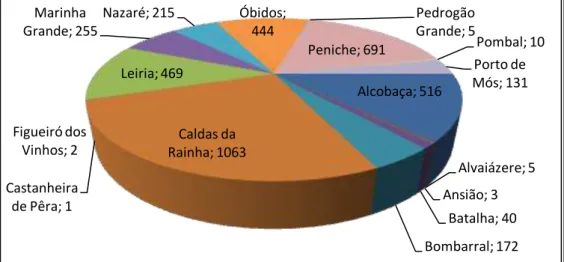
The collection of data necessary to proceed with the empirical research was carried out solely from information available on the Internet. For the compilation of the sample, Portal Casa Sapo was selected. The website chosen has a great coverage nationwide, so that will be used exclusively. Moreover, the use of multiple portals could bias the study, since there might be a risk of repeated observations. The period of data collection took place between the months of October 2010 and December 2010. We proceeded to market segmentation into submarkets, that is, the division was made from observations in 16 submarkets (counties belonging to the district of Leiria). The final sample is composed of 4022 housing, offered for sale, in Portal Casa Sapo , in the district of Leiria. Figure 1 shows the distribution of observations by the analyzed counties.
Figure 1: Distribution of observations by counties Alcobaça; 516 Alvaiázere; 5 Ansião; 3 Batalha; 40 Bombarral; 172 Caldas da Rainha; 1063 Castanheira de Pêra; 1 Figueiró dos Vinhos; 2 Leiria; 469 Marinha Grande; 255 Nazaré; 215 Óbidos; 444 Pedrogão Grande; 5 Peniche; 691 Pombal; 10 Porto de Mós; 131
23
The most represented county in the sample is Caldas da Rainha, followed by Peniche, Alcobaça and Leiria. Counties of Ansião, Castanheira de Pêra, Figueiró dos Vinhos and Pedrógão Grande are sparsely represented in the sample, so there will be difficulties on the convergence for these counties in the regression models.
3.5. Variables definition 3.5.1 Dependent variable
According, Canavarro et al. (2010), Kong et al. (2007) and Morancho (2003), as dependent variable, the offer price by housing available for sale, rather than sale value, was considered.
3.5.2. Independent variables
Independent variables were selected according to the characteristics set of housing, available on the portal Casa Sapo. For inclusion in the model, the transformation of qualitative variables in dummy variables was made.
Table 2:
Definitions and sources of independent variables
Variable Variable name Definition Source Expected sign
on price Structural characteristics
Age Age of housing
The difference between the current year, i.e., 2011, and the year when housing began to be built or restored Goodman and Thibodeau (1997) Negative (-) Hs House Size
Total floor area of one housing in square meters. For estimation of the model we use the useful area
Goodman and Thibodeau (1997)
Positive (+)
CTV Cable TV Dummy=1 if the housing has cable
TV; 0 otherwise Selim (2008) Positive (+)
PL Pool Dummy=1 if the housing has pool;
0 otherwise
Goodman and Thibodeau (1997)
Positive (+)
JZZ Jacuzzi Dummy=1 if the housing has
jacuzzi; 0 otherwise Selim (2008) Positive (+)
SN Sauna Dummy=1 if the housing has
sauna; 0 otherwise Selim (2008) Positive (+)
GRPK Garage or parking Dummy=1 if the housing has
garage or parking; 0 otherwise Pozo (2009) Positive (+) (continued)
24 Table 2 (continued):
Definitions and sources of independent variables
Variable Variable name Definition Source Expected
sign on price Structural characteristics
EQK Equipped kitchen Dummy=1 if housing has equipped kitchen; 0 otherwise
Rodrigues
(2008) Positive (+)
TYP Type of house We include 6 dummy variables
identifying the type of housing a)
Pozo (2009), Morancho (20 03) Selim (2008) Positive (+)/ Negative (-)
BED Number of bedrooms
We include 9 dummy variables identifying the number of bedrooms (1 to 9 bedrooms)
Angli and Gencay (1996)
Positive (+)/ Negative (-)
TRR Terrace Dummy=1 if housing has terrace; 0
otherwise
Maurer et
al. (2004) Positive (+)
US Usage status
We include 5 dummy variables identifying the usage status of housing b)
Rodrigues
(2008) Positive (+)
Location characteristics NRSL Near a river, sea, lake
Dummy=1 if housing is located near a river, sea or lake; 0 otherwise
Wen et al.
(2005) Positive (+)
NFGMP
Near green spaces (field, gardens,
mountains, pine
forest)
Dummy=1 if housing is located near green spaces; 0 otherwise
Morancho
(2003) Positive (+)
CT Housing is located in a particular county
To control for differences in housing prices between counties, we include 15 counties dummy variables c)
Pozo (2009) Positive (+)/ Negative (-)
DWT Downtown or in the city
Dummy=1 if housing has good access to the downtown; 0 otherwise Ozzane and Malpezzi (1985) Negative (-) Neighbourhood characteristics NEF Near entertainment facility (playground, shopping centre, tennis court, gym)
Dummy=1 if housing is located near entertainment facility; 0 otherwise
Wen et al.
(2005) Positive (+)
NPS
Near public services (schools, police station, pharmacy, supermarket, public transportations, health centre, hospital, banks, train, fire-brigade, church)
Dummy=1 if housing is located near public services; 0 otherwise
Wen et al.
(2005) Positive (+)
25 Table 2 (continued):
Definitions and sources of independent variables
Note. a) To represent the type of house variable we use 6 dummy variables TYP_1 (flat); TYP_2 (old house); TYP_3 (cottage); TYP_4 (story home); TYP_5 (housing) and TYP_6 (germinated housing). b) To Usage status Variable we use the following dummy variables: US_un (under construction); US_nw (new); US_tc (to recover), US_rc (recovered) and US_us (used). c) To represent the location of a housing in one of the existent counties (16 counties) at the Leiria district we creat 15 dummy variables: CT_al (Alcobaça); CT_av (Alvaiázere); CT_an (Ansião); CT_bt (Batalha); CT_bo (Bombarral); CT_cr (Caldas da Rainha); CT_fv (Figueiró dos Vinhos); CT_l (Leiria); CT_mg (Marinha Grande); CT_nz (Nazaré); CT_ob (Óbidos); CT_pg (Pedrogão Grande); CT_pe (Peniche); CT_pb (Pombal) and CT_pm (Porto de Mós).
26
4. PRESENTATION AND DISCUSSION OF RESULTS
This section describes and discusses the results. We present the descriptive statistics, and the multiple linear regression model.
4.1. Descriptive statistics
The sample integrates 4022 observations. Tables 3 and 4 provide summary statistics of the dependent variable and independent variables. In the sample, the price has a mean value of € 168 918.00, with a dispersion value of 108 028. The minimum and maximum values are, respectively, € 17 500.00 and € 1 500 000.00. The age has a mean value of 7.55 years, with a dispersion value of 11.65. The minimum and maximum values are, respectively, 0 and 111 years. The house size has a mean value of 183.38 m2, with a dispersion value of 161.82. The minimum and maximum values are, respectively, 20m2 and 2980 m2. In table 4, we present the percentage of each characteristic in the sample.
Table 3:
Summary statistics of dependent variable and continuous independent variables Std.
N Mean Deviation Minimum Maximum
Dependent Variable:
OFFER PRICE 4022 168 918 108 028 17 500 1 500 000
Independent Variables: Structural characteristics:
Age of housing 4022 7.55 11.65 0 111
House size: Floor area (m2) 4022 183.38 161.82 20 2980
Table 4:
Summary statistics of dummy independent variables
N % Structural Characteristics Cable TV 266 6.6% Pool 253 6.3% Jacuzzi 6 0.1% Sauna 10 0.2% Garage or parking 1389 34.5% Equipped kitchen 380 9.4% Terrace 310 7.7% Type of house: Flat 650 16.2% Old house 81 2.0% Cottage 88 2.2% Story home 3 0.1% Housing 2209 54.9% (continued)
27 Table 4 (continued):
Summary statistics of dummy independent variables
N % Structural Characteristics Type of house: Housing geminated 989 24.6% Number of bedrooms: Bed 1 327 8.1% Bed 2 973 24.2% Bed 3 1880 46.7% Bed 4 669 16.6% Bed 5 114 2.8% Bed 6 29 0.7% Bed 7 14 0.3% Bed 8 5 0.1% Bed 9 7 0.17% Usage status: Under construction 547 13.6% New 1725 42.9% To recover 61 1.5% Recovered 72 1.8% Used 1557 38.7% Location Characteristics County: Alcobaça 516 12.8% Alvaiázere 5 0.1% Ansião 3 0.1% Batalha 40 1.0% Bombarral 172 4.3% Caldas da Rainha 1063 26.4%
Figueiró dos Vinhos 2 0.1%
Leiria 469 11.7% Marinha Grande 255 6.3% Nazaré 215 5.3% Óbidos 444 11.0% Pedrogão Grande 5 0.1% Peniche 691 17.2% Pombal 10 0.2% Porto de Mós 131 3.3%
Downtown or in the city 560 13.9%
Near Green Spaces 616 15.3%
Near a River, Sea, Lake 208 5.2%
Neighbourhood Characteristics
Near entertainment facility 772 19.2%
Near public services 1097 27.3%
4.2. Multiple linear regression model
Analytically, our hedonic equation is defined as follows:
i i i i i j j j i i j i j j i i j j j i j j j i i i i i i i i i NPS NEF DWT CT NFGMP NRSL US TRR BED TYP EQK GRPK SN JZZ PL CTV Hs Age Y
49 48 47 , 15 1 31 31 30 5 1 , 24 24 , 9 1 14 , 6 1 8 8 7 6 5 4 3 2 1 0 (4.1)28
Yi is the dependent variable, in this case, the offer price. i represents the ith sample observation in n observations. k are the model parameters that indicate the variation on the expected value of Y, due to the variation of one unit in independent variables, when all the other independent variables in the model remain constant. i is the random term (or perturbation term), which represents all the variables with explainable power over the dependent variable not included in the model. To find “good” estimators of regression parameters, we use the least squares method.
As this is a multiple linear regression model, beyond the inference for each parameter, we must determine if the model is globally significant, through a test of significance of the coefficient of determination (F test), which allows checking if the multiple linear regression model is globally significant. This test, however, does not indicate if all the variables are significant, or which ones are most important; it is, therefore, necessary to apply the t test to determine the significance of each variable in particular.
The coefficient of determination (R2) appears as a measure of the effect of the explanatory variables in reducing the variation of Yi, i.e., in reducing the uncertainty associated with the prediction of Yi. Otherwise, the R2 measures the percentage or proportion of total variation of Yi explained by the model.
Adding more variables to the regression model can only increase the R2. To address this, it is usually suggested a measure that adjusts for the number of independent variables in the model – determination coefficient. The adjustment is simply to divide the two sums of squares by their degrees of freedom. This coefficient can assume a lower value, when introducing an additional explanatory variable, because a reduction in the sum of squared errors can be compensated for the loss of one more degree of freedom in the denominator.
4.2.1. Selection of the best functional form for the regression model
The linear, logarithmic, squared and cubic functional forms were tested, and the quality of the linear fit obtained, with the coefficient of determination (R2) and the adjusted coefficient of determination (Ra2) being used as a criterion to select the best functional form. In these linear regression models, all the independent variables are used.
29 Table 5:
Determination coefficients and functional forms
Model R Square Adjusted R Square
Linear 0.510 0.504
Logarithmic 0.494 0.488
Squared 0.546 0.540
Cubic 0.553 0.547
The quality of the obtained fit is better for the cubic functional form, with R2 = 55.3%, followed by the squared functional form, with R2 = 54.6%, being the quality of the adjustment lower for the linear (R2 = 51.0%) and logarithmic (R2 = 49.4%) functional forms. Among others, see Anglin and Gengay (1996) with R2 = 68.7%, Ozanne and Malpezzi (1985) with R2 = 56% and Pasha and Butt (1996) with R2 = 54.1%. The same remarks can be made upon the comparison of the adjusted coefficient of determination. Thus, we can easily conclude that the cubic functional form should be used. In the cubic functional form, we will use the dependent variable price and our hedonic equation is now defined as follows:
i i i i i j j j i i j i j j i i j j j i j j j i i i i i i i i i i i i i NPS NEF DWT CT NFGMP NRSL US TRR BED TYP EQK GRPK SN JZZ PL CTV Hs Hs Hs Age Age Age Y
53 52 51 , 15 1 35 35 34 5 1 , 28 28 , 9 1 18 , 6 1 12 12 11 10 9 8 7 3 6 2 5 4 3 3 2 2 1 0 (4.2)The cubic functional form has been used, for example, by Goodman and Thibodeau (1995) for capturing the effects age. We will have two types of reading in the cubic functional form:
For continuous independent variables, the rate at which an amenity adds to the price of a house does not stay constant, and can change at a rate that, it self, varies. For example, a case of decreasing additional returns followed by increasing additional returns. This would visually represented by an approximate S-shaped curve;