On long-run price comovements between paintings and prints

(1)

ISSN 0104-8910

ON LONG-RUN PRICE COMOVEMENTS BETWEEN

PAlNTINGS AND PRlNTS

Corinna Czujack, Renato Flôres e Victor Ginsburgh

(2)

On long-run price comovements between

paintings and prints

1

Corinna Czujack, Renato Flores and Victor Ginsburgh CEME, Université Libre de Bruxelles

July 1995

1 Introduction

The art market is the result of complex interactions, most of which can hardly be explained by economic theory. Signals such as the name of an artist, specificities of diHerent media, reactions of art galleries, critics, mu-seum directors and investors exert a large variety of influences on prices and values, which are difficult to model with accuracy.

It is however possible to address interesting questions, using sales prices as the basic information on values and relative scarcities. Indeed, if prices can be taken as synthesizing all the effects just mentioned, their dynamic interactions across artists and media may reveal some common patterns or, on the contrary, call attention to divergent behaviours. Both may turn out to be explainable by art history or aesthetical judgements. If so, further evi-dence would have been provided by a more quantitative analysis; otherwise, new directions for research could be opened.

In particular, if one accepts the idea of "a global market" for say, post-impressionnist paintings, one may ask whether artists like Braque or Picasso lead or follow this global market. One may also examine whether prices of prints and paintings for a given artist follow a common pattern; if so, one may construct portfolios of prints, which are cheaper, more liquid and probably less risky than portfolios of paintings.

In this paper, we try to answer questions of this type, using the infor-mation contained in prints' and paintings' price indices for global markets and for some individual artists who have been active both as painters and as lithographers or etchers - Braque, Chagall, Ernst, Miró and Picasso.

The analysis is carried out by estimating vector autoregressive models, using the techniques developed by Johansen (1988, 1991) and Johansen and

1 A previous version of this paper was presented at the conference Approches Compar-atives en Economie de la Culture, Paris, May 1995. We thank Ruth Towse and other participants for comments.

(3)

Juselius (1990, 1992). These methods make it possible

(i) to estimate possible steady-state relations between prices and isolate long-run from short-run behaviour, and

(ü) to test for exogenenous behaviour in an error-correction model setting. Though this methodology is known to many economists, it is much less widespread in the field of cultural economics.2 Therefore, Section 2 is de-voted to the basic framework and to the key concepts used in the paper.

Section 3 briefiy discusses the construction of the price indices on which our study is based. In Section 4, we analyze three kinds of relationships: (i) between the market for paintings and the market for prints (Section 4.1); (ii) between each individual artist and the global market for prints (Section 4.2);

(iü) between the print markets for the five artists (Section 4.3).

The discussion is kept informal, but the more technical details can be found in the Appendix. Section 5 concludes the paper.

In broad terms, we find that prices of prints and paintings have a common trend, but prints yield lower long-run returns. Relations between individual artists and the global market for prints vary from one artist to the next, but again, the series have common trends. Though each of the five artists is unique by himself, a separating line can be drawn between Braque-Ernst, and Chagall-Miró-Picasso. In particular, Picasso, as expected, plays a major role and Chagall, though being very connected to the others, behaves quite differently from them.

2 Cointegration and exogeneity

2.1 The error-correction model

Cointegration3 is loosely related to the concept of stationary linear combina-tions of nonstationary processes. Suppose that the interest lies in studying

I nonstationary time series of prices Yi,t, i

=

1,2, ... , I,

t

=

1,2, ... , T. Under certain conditions, it is possible to estimate the coefficients of the following

2See however Ginsburgh and Jeanfi1s (1995).

3In this section, we present an informal discussion of the key concepts that will be econometrically tested in this paper. The interested reader should go to the papers cited for a rigorous view on the subject. Chapters 2 and 3 in Urbain (1993) aIso provide a good insight on the issues.

(4)

system of equations:

J K I

tl.Yi,t

=

L

ai;Z;,t-l

+

L L

'Yii',ktl.Yi',t-k

+

'YiO

+

ei,t, i

=

1,2, ... , l. (1)

;=1 k=I~=1

Dne of the conditions is that the tl.Yi,t are stationary. The other is that the variables:

I

Z;,t =

L

(3i;Yi,t, i=1

j

=

1,2, ... , J :::; l - 1, (2)

obtained as linear combinations of the original Yi,t variables, are also sta-tionary. These last equations are calIed "long-run" or "steady-state" rela-tionships.

The parameters ai; in (1) measure the speed at which deviations from the steady-state are corrected, so that the mo dei is often refered to as an error correction mechanism (ECM). The vectors ({31,;,

132,;, ... ,

(3I,;),j = 1,2, ... , J

are calIed cointegrating vectors. The terms:

K I

L L

'Yii',ktl.Y~,t-k

+

'YiO (3)

k=1 i'=1

describe the short-run dynamics. The number of lags (K) should be chosen in such a way that the error processes ~t, i = 1,2, ... , l, are Gaussian white noise.

Form (1) is fairly general and some special cases can readily be obtained; in particular, it may happen-(a) that no cointegrating vectors exist, (b) that some or alI of the ai; coeflicients are zero, (c) that some or alI of the 'Yii' ,k

coeflicients are zero. These special cases wiIl be discussed in Section 2.2. Note that the ai; 's and the {3i; 's are undetermined up to scalar multi-plication; this explains why system (1) can also be written as:

I K I

tl.Yi,t =

L

7rWYi',t

+

L L

'Yii',ktl.Y~,t-k

+

'YiO

+

ei,t, i = 1,2, ... , l, (4)

~=1 k=l~=1

where the S<rcalIed impact coeflicients 7rii' are now uniquely determined. Note also that in the case of a two-variable system, there wiIl exist at most one cointegrating relation which, after suitable renormalization, can be written as:

(5)

~ -- - - -- - - ,

This implies that Ou should be negative and 021 positive. The reason is that, if in (5) ZI,t is positive, Yl,t is "higher" than its equilibrium value, so that the error-correction mechanism acts in lowering its next value and this entails Ou

<

O. A similar reasoning applies to 021.

Estimating model (1) for price indices of painters or media, allows us to obtain an insight on the joint short-run dynamics of the series. As pointed out, the long-run or steady-state term, present in these equations, acts in correcting the short-run deviations back to the "ideal" long-run equilibrium. Finding cointegration, say between paintings and prints by a specific artist, is a nontrivial fact because it implies that, in the long-run, the price series do not diverge and also that their short-run variations are infiuenced by this long-run equilibrium. In other words, this means that the series have a common nonstationary movement, which is eliminated in the cointegrating relation.

2.2 Exogeneity and causality

The issues of exogeneity and causality often appear in econometric mod-elling involving several variables. Though intuitively simple, the concept of exogeneity can have difIerent shades, as pointed out in the seminal paper by Engle et alo (1983). For our purposes, and in the context of model (1), a variable wiIl be weakly exogenous for a set of parameters if, conditioning the model with respect to that variable, no useful sample information for inference on those parameters is lost.

In the case of the ECM-model, the concept has some fine connotations. Consider a given equation, ~ay the first. It might happen that Ou is equal to zero; this would mean that the corresponding cointegration relationship ZI,t-l does not play any role in explaining the behaviour of the (difIerenced) price index Yl,t. If all 01j'S are zero, we say that the behaviour of Yl,t is weaklyexogenous4 _{with respect to the long-run relationships and (1) can be}

written as:

K I

6Yl,t =

L L

'"rli',k 6 Yi',t-k

+

'"rIO

+

el,t·

k=1 i'=1

(6) As a result, the system can be separated into two subsystems. The first comprises the equations corresponding to the weakly exogenous variables, while the second is formed by the remaining ones. Making the link with the 4This idea has received a finer treatment by Mosconi and Gianini (1993), which will

not be used in this paper.

(6)

informal definition of weak exogeneity stated above, as far as the long-run relationships are concemed, we can condition the second subsystem with respect to the first one, Le. we can study the behaviour of the indices in the second subsystem for each "fixed" set of values of the weakly exogenous variables. Note that performing the reverse would be meaningless, as the variables of the second subsystem do not convey any long-run information to the ones in the first subsystem.

Contrary to exogeneity, the concept of causality builds on ideas from common language and philosophy. In our context, causality will be defined in the lines of Granger (1969): Xt will (Granger-) cause Wt if and only if the

past of Xt influences Wt, but the opposite is not true. The "past" is here

understood as the collection of lagged values of Xt, influences being measured

in terms of linear regressions.

Weak exogeneity plus Granger causality makes for what Engle et alo (1983) suggested to call "strong exogeneity." It is evident that a group of variables (here, price indices) may be weakly but not strongly exogenous. This is easily seen if one remembers that lagged differences of all the indices appear in principIe in the short-run part of the equations in (1). For weakly exogenous variables to be strongly exogenous, it must be that the short-run behaviour of the other variables do not Granger-cause them, Le. that they do not appear in their equations. For example, Yl,t will be strongly exogenous, if the first equation of system (1) can be written as

K

L).,Yl,t =

L

1'll,kL).,Yl,t-k

+

1'10

+

el,t·

k=1

(7)

No other variable than the past of Yl,t itself contributes in explaining Yl,t.

2.3 Efficiency and returns

If, in addition to exogeneity of say, Yl,t, we find that there is no influence of the short-run either, and that 1'10 is not significantly different from zero, we are left with the following equation:

L).,Yl,t = el,t (8)

and the L).,Yl,t series is a random walk.

Given that Yl,t is a price series, (8) means that the underlying market is "weaklyefficient:" in the context of the model, no variable (contemporaneous

(7)

or past) has an influence on Yl,t and the current price is the best forecast for next period's price.

In the case of a two-equations system, there is also an interesting financiaI interpretation of the long-run relation. Taking the expectation of the first-difference of (5), we have:

(9) If the price series are expressed in logarithms, the differenced series represent returns, so that (9) gives a relationship between the two expected returns. If {3

>

1, (long-run) returns from Yl,t are higher than those generated by Y2,t. Since riskier assets yield higher returns, Yl,t should probably relate to an asset that is riskier than Y2,t. Note that if

f3

= 1, the expected returns of the two assets are equaI.

Finally, consider a two-equations ECM in which the first price series is weakly eflicient, while in the second equation, the long-run term is present. This means that differences in the first series are merely white noise, while in the second, some short-term forecasting is possible. It is then reasonable to expect that the first asset should provide higher returns, since it is riskier than the second one. This hypothesis can be tested on the

f3

coeflicient, which should be larger than one.

3 The data

3.1 PrincipIes or construction or the price indices

The price indices used in out calculations have been computed through he-donic regressions, as suggested in Chanel et aI. (1992). One estimates the following equation:

m

Pi,t =

L

akXik,t

+

c(t)

+

~i,t. k=l

(10)

In this equation, Pi,t is the (logarithm of the) price of a collectible i sold at time

t,

Xik,t is a time-variant idiosyncratic attribute of collectible (i,

t);

c(t)

is the market-wide price effect and ~i,t is an error termo Model (10) can be given a convenient interpretation if one isolates in the right-hand side the time effect and the random error. The left-hand side can then be thought of as representing the price of a work i sold in t, freed from the implicit prices of its characteristics. This "characteristic-free price" is assumed to include the

(8)

- - - ---.--- - - - -

-effect of time and a random error onlyj by averaging the characteristic-free prices of alI works i sold in t (or, equivalently, by regressing these prices on time dummies), one obtains the average price of a "standardized" work at time t. The specification of c(t) considered in that case is:

TT

C(t)

=

L

<Pt

6

t,

(11) t='Tb

where

[ro,7']']

is the time interval over which observations are availablej 6t

is a dummy variable which takes the value one if work i is sold in period t E

[ro,7']'],

and

zero

otherwisej the

<Pt'S

are parameters to be estimated. The sequence

[<p'Tb'

<PTlI ••. , <PTT]

is used to construct the price (or the value) index Yt.

Most of the work carried out in order to compute returns on art, uses repeat sales regressions (Le. regressions based on observations of collectibles sold at least twice) rather than hedonic regressions. The pros and cons of both methods are discussed in Chanel et alo (1992) and Ginsburgh (1994).5 Here, we merely note that it would be impossible to construct yearly (or half-yearly) indices using repeat sales only, since the number of resales for which prices are observed is quite limited.6

3.2 Original data available

The data used to calculate value indices are taken from Mayer's Annuaire

des Ventes (1963 to 1994). These yearbooks of public auctions are available

since 1963 (sales of 1962)j we thus cover the years 1962 to 1993. Two databases were compiled, one for paintings and one for prints. The first contains 25,073 sales for 84 well-known artists, selected in a fairly subjective way.7 The database for prints contains 10,028 sales for 25 artists.

In addition to global price indices based on the 84 and 25 artists respec-tively, we also constructed indices for five artists for whom the number of sales was large enough: Braque (359 paintings and 681 prints), Chagall (341 and 1,943), Ernst (435 and 280), Miró(288 and 1,708) and finally, Picasso (826 and 3,132).

In Mayer's compendia, each sale is described by a certain number of characteristics (see below) and by a sale number, corresponding to a specific

5See also Goetzmann (1990, 1993).

6This is certainly the case for paintings, but much less 50 for prints. See Pesando (1993).

(9)

auction describing the location and the date of the sale. It is therefore possible to construct semi-annual, quarter1y or even monthly price indices. The relatively smali number of salesB made us opt for semi-annual indices, taking the years 1962 to 1966 as base period.

The characteristics of the artworks are different for paintings and for prints. Those that describe paintings are rather limited; beside the name of the artist (and the title of the painting), the yearbooks provide only a very rough description: the size of the work (height and width), the year in which it was painted, the medium used, the place of the sale (saleroom, country) and the year of sale. Such a simple description is however hardly comprehensive enough to explain the price differences between artists and one is necessarily led to include some measure of the repute of the painter. We chose to work with dummy variables for artists.

The characteristics for prints are more numerous. Beside the name of the artist, the size of the work, the year of production, the medium used, the place of the sale (saleroom, country) , and the year of the sale, Mayer provides information concerning the technique used (etching, lithography, etc.), the type of paper (Arches, Chine, etc.), the fact that the print is black and white or coloured, the signature, some specials (épreuve d'essai, épreuve d 'artiste, etc.), the total number of copies and the number of the copy sold.9

Moreover, for the five individual artists considered and given that the year of production is (very often) available, it was possible to introduce dummy variables for the different "creation" periods (e.g. for Picasso, the "blue," the "pink," the "cubist" period, etc.), which are usually priced very differently.lO

Prices are given in current French francs by Mayer, who uses the ex-change rate prevailing during the day of the sale.

3.3 Indices constructed

The model we use combines (10) and (11) and is estimated on the fuH sample of sales and resales. Regressions were thus run for ali artists together 8Especially for the period 1962-1972, during which there are 50metimes less than ten observation per year for a given artist.

9See also Table 1, for more details.

l°lt is obviously difticult to define these periods (painters have seldom changed their style suddenly: changes occur gradually, and painters may also simultaneously paint in different styles) 50 that the indications given in the various art history books do not necessarily coincide. We have used Laclotte and Cuzin (1989). The authors are respectively Chairman and Chief Curator of the paintings department at the Musée du Louvre.

(10)

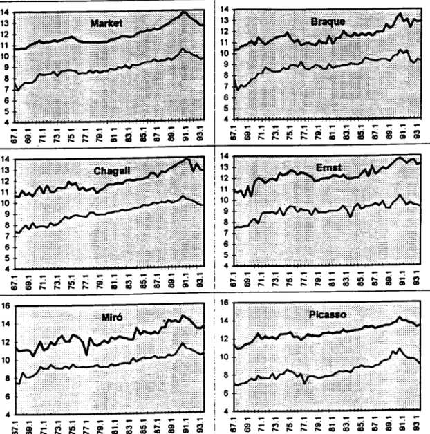
to obtain the "market" index as well as individually for Braque, Chagall, Ernst, Miró and Picasso. The indices are then defiated, using the French consumer price indexo They are reproduced in Figure 1.

3.4 Overall quality of the regression results

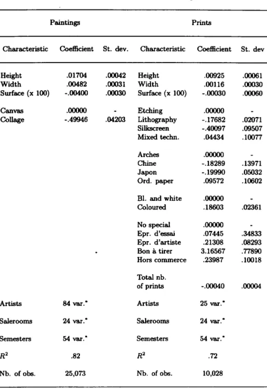
We illustrate the results with two regressions for paintings and for prints, run on the full sample (these are the regressions used to obtain the "market indices"). As can be seen from Table 1, the fit is quite good in both cases. All the coefficients (with the exception of the "paper" medium for prints, which should probably be negative) have the expected signo

4 Empirical results

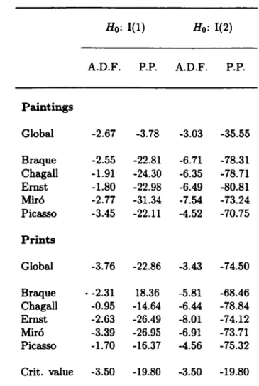
The analysis is split into three parts. First, we look for cointegration between prices for prints and paintings for the market as a whole, as well as for each of the five artists individually. We then examine the market for prints only and test whether prices for each artist are cointegrated with the global price indexo Finally, we construct a system of five equations (the price indices for the five artists') for prints and investigate their relations. Before setting up these models, we tested whether (the logarithms of) the price series used are integrated of order one, so that their first differences are stationary. The results of these tests, given in Table AI in the Appendix, indicate that alI series, with the exception of the global indexes can be considered as integrated of order one, at the 5% leveI. The global indexes also show evidence of a single unit rooJ; at the 10% leveI.

4.1 Cointegration between prints and paintings

We investigate the conjecture that the markets for paintings and prints -both globally and for each artist individually - move together in the long-run. We estimate in each case the following two-equations system:

K 2

fl.Yi,t

=

Oi(.81Yl,t-l +.8'2Y2,t-l)+

L L

T'ii',kfl.Yi',t-k+T'iO+ei,t, i

=

1,2 (12)

k=li'=1

where different values for K, the number of lags for short-run effects (in-cluding no lag at all), have been tried out and

.81

is normalised to unity.

Since only twO variables are considered, there exists at most one cointe-grating vector. The first and second equations concern paintings and prints,

(11)

-Table 1 Some results from the hedonic regressions

Paintings Prints

Characteristic Coeflicient St. devo Characteristic Coeflicient St. dev

Height .01704 .00042 Height .00925 .00061 Width .00482 .00031 Width .00116 .00030 Swface (x 1(0) -.00400 .00030 Swface (x 1(0) -.00030 .00060 Canvas .00000 Etching .00000 Collage -.49946 .04203 Lithography -.17682 .02071 Silkscreen -.40097 .09507 Mixed techn. .04434 .10077 Arches .00000 Chine -.18289 .13971 Japon -.19990 .05032 Ord. paper .09572 .10602 BI. and white .00000

Coloured .18603 .02361 No special .00000 Epr. d'essai .07445 .34833 Epr. d'artiste .21308 .08293 Bon à tirer 3.16567 .77890 Hors commerce .23987 .10018 Total nb. ofprints -.00040 .00004 Artists 84 var." Artists 25 var.·

Salerooms 24 var: Salerooms 24 var." Semesters 54 var.· Semesters 54 varo

.

R2 _.82 _R2 _.72

Nb. ofobs . 25,073 Nb.ofobs. 10,028

• For obvious reasons, we do not give the coefficients here. F-testa have been run and show that the coefficients within groups (artista, salerooms and semesters) are not equal.

(12)

respectively. The results are summarized in Table A2 in the Appendix, where a more technical discussion can also be found. The main findings follow.

The global market

For the global market, i.e. the one represented by the price indices pooling together many artists, the fitted model is:

6Yl,t = el,t

6Y2,t = 0.37(Yl,t-l - 1.24Y2,t-I)

+

e2,t·

This shows that, with respect to prints, paintings are weakly efficient: their short-run returns follow a white noise processo Therefore, as expected, their long-run returns are almost 25% higher than those of prints. Short-run re-turns for prints are corrected by the cointegration relationship: whenever the price for prints is higher than 0.81 (i.e. 1/1.24) times the price for paint-ings, the print index falls - on average - by 37% of the difference between Yl,t-l and 1.24Y2,t-l.

Individual artists

For individual artists, the results follow either of two patterns. In the case of Braque and Ernst, prices of paintings are also weakly exogenous, but short-run lags appear in both equations, 50 that weak efficiency of paintings does not apply.

For Chagall, Miró and Picasso - though no short-run lags were found to be significant -, no index is weakly exogenous with respect to the long-run relation. For Chagall, the model is:

6Yl,t = -0.35(Yl,t-l - Y2,t-I)

+

el,t

6Y2,t = 0.14"(Yl,t-l - Y2,t-I)

+

e2,t

showing that long-run returns for prints and paintings are identical. For Picasso, long-run returns for prints are even higher than for paint-ings, as shown by bis equations:

6Yl,t = -0.39(Yl,t-l - 0.71Y2,t-d

+

el,t

(13)

This result is probably a consequence of the very high prices that are already obtained for Picasso's paintings.

4.2 Prints: cointegration between individual artists and the

global market

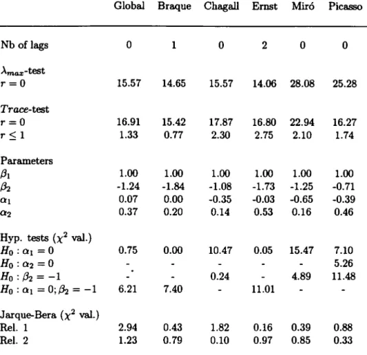
Here, we are interested in the relations between prices of prints for individual artists and the print market as a whole. We estimate a system similar to (12), where now the first equation is related to the artist and the second to the global market. Detailed results are given in Table A3 in the Appendix.

In Braque's and Ernst's cases, the global market is weakly efficient. Prints by these two artists have a lower long-run return than the one given by a notional portfolio, identical to the one used to construct the global indexo In the case of Braque, for example, the model is:

~YI,t = -O.51(YI,t-1 - O.87Y2,t-l)

+

el,t,

~Y2,t = e2,t·

For Chagall,l1 Miró and Picasso, the cointegrating relation influences the global index, and their long-run returns are higher than those of the indexo Picasso's prints are weakly efficient, and the final model fitted for him is:

~YI,t = el,t,

~Y2,t = O.20(YI,t-1 - 1.39Y2,t-d

+

e2,t·

Picasso prints can be thus considered as "leading" or "pushing" the mar-ket. Their long-run returns are 39% higher than those of the notional print portfolio. Moreover, if the global print index falls to leveis below 1/1.39 times the Picasso prints index, global short-run returns will have a higher probability of being negative.

4.3 Prints: cointegration between individual artists

We now consider the system of five equations in which only prices of prints for the five artists appear. The order is Braque (subscript B), Chagall (C), Ernst (E), Miró (M) and Picasso (P). Given our previous findings, we assume that Picasso's prices are weakly exogenous and we set to zero the

11 According to the >'maz-test, there is no cointegration at the 5% levei.

(14)

-OP,j coefficients in Picasso's equation. We then try to determine:

(i) who are the artists contributing to the long-run relationship(s) and who are the weakly exogenous ones;

(ti) are there artists who are strongly exogenous;

(m) what is the most parsimonious model to describe the five artists' short-run behaviour.

A technical discussion is provided in the Appendix, together with Tables A4 and

A5.

The findings are as follows.

Chagall and Miró may be left out from the long-run cointegrating rela-tionship. They thus follow long-run trends which are different from those of Braque, Ernst and Picasso. Therefore, it was interesting to check whether Chagall's and Miró's short-run lagged values could also be left out of the three other artists' equations. li so, this would indicate that neither the long-run nor the short-run of the former exerts any influence on the group of the latter, so that Braque, Ernst and Picasso would be strongly exoge-nous. However, this happens to be the case for Braque and Ernst, but not for Picasso, whose prices are partly explained by those of Miró.

The final, more parsimonious fitted model is:12

LlYB,t

= -

O.33z1,t - 0.49z2,t

+

eB,t

LlYc,t = - O. 17z1,t

+

O.06Z2,t - O.58LlYc,t-l

+

O.26LlYM,t-l

+

eC,t LlYE,t

=

1.02Z1,t - O.08Z2,t

+

eE,t

LlYM,t = O.05Z1,t - O. 26Z2,t

+

eM,t

LlYP,t = - 0.41LlYB,t-l

+

0.40LlYM,t-l - O.36Llyp,t

+

ep,t·

5 Conclusions

The analyses performed reveal that the prices of the five artists studied behave differently. We first have Braque and Ernst, who show a "follow the market" , more classical behaviour: the global prints index is, in both cases, weakly exogenous. The same holds if the global prints index is replaced by the paintings index of the artist.

The other three artists stand out as special individualities. For alI three, the paintings and prints markets are interrelated. Chagall is perhaps the most singular case. The other four are strongly exogenous w.r.t. him, in the joint, five artists' prints model. Moreover, his index for prints is the only 12This parsimonious representation is based on the model of Table A5, dropping the short-run coeflicient which are not significantly different from zero.

(15)

one that presents weaker e\"idence of being cointegrated (only at the 10% leveI) with the global indexo Everything seems to indicate that Chagall has a very special market of his own, in which prints as well as paintings are equally rewarding in the long-run.

Picasso is, naturally, the other singularity. He alone seems to be weakly exogenous in the prints market. Indeed, his price index is weakly efficient with respect to the global index, and he is the artist whose prints generate higher long-run returns than his paintings.

Miro prints are interrelated with the market, and their formal interrela-tionship with those of Picasso seems to corroborate a well-known historical facto

Finally, in financial terms, investing in prints the prices of which are weakly efficient would be a bad choice for speculators. These should go for prints whose price changes can be forecasted by exogenous variables which may signal - as fundamentais - the direction of the changes. On the other hand, the closer the indices are to efficiency, the higher is their (long-run) return (with respect to the other ones), given that they constitute riskier assets. As a consequence, buying prints by these artists is a good choice for long-run investors.

6 References

Anderson, R.C. (1974), Paintings as an investment, Economic Inquiry 12, 13-25.

Chanel, O., L.-A. Gérad-VEp"et and V. Ginsburgh (1992), The relevance of hedonic price indices: the case of paintings, manuscript.

de la Barre, M., S. Docclo and V. Ginsburgh (1994), Returns of Impres-sionist, Modern and Contemporary European Paintings, 1962- 1991,

Annales d'Economie et de Statistique 35, 143-181.

Engle, R.F.; D.F. Hendry and J.F. Richard (1983), Exogeneity,

Economet-rica 51, 277-304.

Ginsburgh, V. (1994), Objective properties of art and its price, paper pre-sented at the Annual Meeting of the Midwest Economics Association, Chicago, March.

Ginsburgh, V. and P. Jeanfils (1995), Long-term comovements in interna-tional markets for paintings, European Economic Review 38, 538-548.

(16)

Goetzmann, W.N. (1990), Accounting for taste: an analysis of returns over three centuries, First Boston Working Paper Series FB-90-11, November.

Goetzmann, W.N. (1993), Accounting for taste: art and financial markets over three centuries, American Economic Review 83, 1370-1376. Granger, C.W.J. (1969), Investigating causal relations by econometric

mod-eis and cross-spectral methods, Econometrica 37, 424-438.

Johansen, S. (1988), Statistical analysis of cointegration vectors, Journal

of Economic Dynamics and Control12, 231-254.

Johansen,S. (1991), Estimation and hypothesis testing of coointegration in Gaussian vector autoregressive modeIs, Econometrica 59, 1551-1580. Johansen, S. and K. Juselius (1990), Maximum likelihood estimation and

inference on cointegration - with applications to the demand for money,

Oxford Bulletin of Economics and Statistics 52, 169-210.

Johansen, S. and K. Juselius (1992), Testing structural hypotheses in a multivariate cointegration analysis of the PP and the UIP for the UK,

Journal of Econometrics 53, 211-244.

Laclotte, M. and J.-P. Cuzin (1989), Dictionnaire de la Peinture, Paris: Librairie Larousse.

Mayer, E. (1963-1994), Annuaire International des Ventes, Paris: Editions Mayer.

Mosconi,

R.

and C. Gianini (1993), Non-causality in cointegrated systems: representation, estimation and testing, Oxford Bulletin of Economics

and Statistics 55, 399-417.

Pesando, J.E (1993), Art as an investment. The market for modem prints,

American Economic Review 83, 1075-1089.

Urbain, J.-P. (1993), Exogeneity in Error Correction Models, Berlin-Heidelberg: Springer Verlag.

(17)

14 13 12 11 10 9 8 7 6 5 4

_...

.-:

...

,..;

_I

_;::: f"Í lI'i ,..;

_f!!

CD

...

... ...

; ₁₄ ; , ₁₃ , ! 12 11 , , ₁₀ : 9 , ₈ 7 6 5 ; ₄ .- .-: .- .-

...

.-,..; ai .- f"Í lI'i ,..; ai CD CD

... ... ... ... ...

16 14 12 10 8 6 4 .-: .-: .- .-

.-...

ai .- f"Í lI'i

...

ai CD co

... ... ...

... ...

14 13 12 11 10 9 8 7 6 5 4

...

.-:

...

.-:

...

c;

_:3

~

...

ao

I

ãi ljj ,..; CD

I

...

f"Í lI'i

... ...

,..; 14 13 12 11 10 9 8 7 6 5 4 .-: .-

...

.-:

...

.-: .-

...

.-c; f"Í lI'i ,..;

_!li

_ãi f"Í ,..; _lB .- f"Í lI'i ,..;

CD ao ao GI CD

...

10 8 6 4 .-: .-:

...

.- .-:

...

.-: .-: .- .-

...

c; (O) li)

...

m

ãi f"Í

...

a; .- f"Í lI'i ,..; CD ao ao GI co co

... ... ...

...

Figure 1 DeHated prices, in logarithms (fat line: paintings; thin line: prints)

...

.-:

ai _c;

_:3

_~,..;

_!li

_ãi (O)

...

CD GI

.-

...

.- .- _.-:

ai _c; f"Í lI'i ,..; ai _ãi (O)

...

ao CD CD CD GI

...

.-:

...

.-:

ai _c; (O) lI'i

...

a;

ãi (O)

(18)

7 Appendix

7.1 U nit root testing

Table AI presents the results for the augmented Dickey-Fuller and the Philipps-Perron tests. At the 5% probability leveI, the first test accepts the unit root null hypothesis in alI cases, except for the global prints indexo The second test rejects the null hypothesis in several cases. When applied to first-order difIerences, the Philipps-Perron test clearly rejects the second unit root in all cases; this root is however accpeted for both global indices by the Dickey-Fuller testo At the 10% probability leveI, the unit root null hypothesis is accepted in all cases by the ADF testo

7.2 Relations between paintings and prints

Table A2 presents the results, which are now also briefly discussed.

Cointegration relationships. At the 5% probability leveI, cointegration is

accepted by both tests in all cases. We may conclude that there exists a long-run relationship and that prices move together.

Number of shorl-run lags. The "optimal" number of lags is based both

on the Jarque-Bera test and the existence of cointegration. As can be seen,

K varies from one case to the other, but in four instances it is zero and the relationships are:

f).Yi,t

=

Oi(,8~Yl,t-l

+

!h.Y2,t-l)

+

ei,t, i

=

1,2.

Weak exogeneity of paintings. To check this hypothesis, we ran a test Ho : 01

=

O. If this assumption is accepted, the equation for paintings can be

written:

K 2

f).Yl,t =

L L

"fli',kf).Yi',t-k

+

"fIO

+

el,t·

k=1 i'=1

The hypothesis is accepted for the market as a whole, for Braque and for Ernst. It is rejected in the case of Chagall, Miró and Picasso.

Error correction mechanisms. In order for the equations to represent error

correction mechanisms, we must have 01 ~ O and 02 ~ O. This is verified in

(19)

the short-run, any over- or undershooting of prices is corrected.

On the proportionality of comovements. If the hypothesis Ho :

Ih.

= -1 is accepted, the ratio of prices is equal to unity and ex:pected long-run re-turns are the same. This assumption is accepted only for Chagall. For the global market, as well as for Braque, Ernst and Miró, prints have smaller re-turns than paintings. Picasso, is an ex:ception to this rule, and significant1y so, since his

Ih.

is much smaller than one.13

Weak efficiency of the market for paintings. For the global market, (i) prices of paintings are weakly exogenous (i.e. aI = O) and (ii) there are no lags in the short-run part of the relationj moreover, Ho : 1'10 = O is accepted, so that the global market for paintings is weakly efficient.

Retums on prints vs. retums on paintings. For the global market as well as for Braque and Ernst, the equation for prints includes the error-correction term, while for paintings it does not, so that, as discussed in Section 2.3, prints should have a smaller return than paintings and this is actually the case. Prints also have a smaller return than paintings for Chagall and Miró, while for Picasso, the opposite is true.

7.3 Prints: relations between individual artists and the global

market

Table A3 gives the results for the tive pairs. Cointegration is rejected at the 5% leveI for Chagall by ~he Àmax-test, but accepted by the Trace-test.

Cointegration is accepted at the same probability leveI for all other artists. For the remainder, the interpretation of the results can be made along the same lines as in section 7.2.

7.4 Cointegration between the five artists

As can be checked from the results of Table A4, both tests accept cointe-gration.

13Note that if Ho : 01 = O is accepted, we run a joint test Ho : 01 = O, Ih = -1; otherwise, we only run a test {32

=

-1.

(20)

The long-run relationship(s). The long-run cointegration relationships read:

Zj,t

=

{3BjYB,t

+

{3CjYC,t

+

{3EjYE,t

+

{3MjYM,t

+

{3PjYp,t, j

=

1,2, ... , J,

with J :$ 4. Both the Àmaz and the Trace-tests show that there are at most two cointegrating relations (at the 5% leveI), for 0:$ K :$ 3, where K is the number of short term lags. For K = 4, there is only one such relationship.

We are interested in relationships that are parsimonious, and contain a number of individual artists that is as small as possible. We tried all combinations excluding three artists from the above long-run relationship. As is seen from Table A4, the hypothesis is strongly rejected at the 5% probability leveI, whatever the number of lags in the short-run part of the relations. We then turned to test the exclusion of all possible couples of artists and found that, for

K

=

1, the hypothesis {3Cj

=

(3Mj

=

O could not be rejected at the usual 5% leveI. 14

This leads to accepting the following two long-run relationships:

Zl,t = YB,t - 1.32YE,t

+

O.04YP,t

and

Z2,t = YB,t

+

O.09YE,t - O.59YP,t,

in which Chagall and Miró do not contribute to the long-run.

The short-run relationship(s). In Table A5, we give the short-run behaviour for K = 1. Recall that Picasso is assumed to be weakly exogenous from the start. Given that only ~raque, Ernst and Picasso enter the long-run relations, we tested for strong exogeneity of these three artists. Table A5 shows the complete results for the short-run part (with K = 1). Though Chagall's and Miró's lagged price differences are not significant in the equa-tions for Braque and Ernst - and for Miró himself - (as can be seen from the last column of Table A5, HO/'"'fiC.l = '"'fiM,l = O is accepted), Miró's short run behaviour influences Picasso's - which is not too surprising, given the connection between their works. This means that the four other artists are strongly exogenous for Chagall.

14Note that when three artists are excluded, there can be at most one cointegration relationship, 50 that the X2 variable use<! to test the null hypothesis for exclusion of three artists has 3 d.f. When two artists are excluded, there may be one or two cointegrating relations, 50 that the X2-test has 2 or 4 d.f.

(21)

Table AI Unit root tests for the (logged) price series Ho: 1(1) Ho: 1(2) A.D.F. P.P. A.D.F. P.P. Paintings Global -2.67 -3.78 -3.03 -35.55 Braque -2.55 -22.81 -6.71 -78.31 Chagall -1.91 -24.30 -6.35 -78.71 Ernst -1.80 -22.98 -6.49 -80.81 Miró -2.77 -31.34 -7.54 -73.24 Picasso -3.45 -22.11 -4.52 -70.75 Prints Global -3.76 -22.86 -3.43 -74.50 Braque • -2.31 18.36 -5.81 -68.46 Chagall -0.95 -14.64 -6.44 -78.84 Ernst -2.63 -26.49 -8.01 -74.12 Miró -3.39 -26.95 -6.91 -73.71 Picasso -1.70 -16.37 -4.56 -75.32 Crit. value -3.50 -19.80 -3.50 -19.80

A.D.F.

=

augmented Dickey-Fuller; P.P.

=

Philipps-Perron. Ali tests include a constant term and a time trend. The criticai values shown reCer to the 5% probability leveI.

20

FUNDAÇÃO GFT::lUO VARGAS Biblioteca f\!i;.'l",,,,;; .' Simonsen

(22)

Table A2 Cointegration between paintings (ReI. 1) and prints (ReI. 2)

Global Braque Chagall Ernst Miró Picasso

Nb of lags O 1 O 2 O O Àmaz-test r=O 15.57 14.65 15.57 14.06 28.08 25.28 Trace-test r=O 16.91 15.42 17.87 16.80 22.94 16.27 r:::; 1 1.33 0.77 2.30 2.75 2.10 1.74 Parameters /3} 1.00 1.00 1.00 1.00 1.00 1.00

Ih

-1.24 -1.84 -1.08 -1.73 -1.25 -0.71 o} 0.07 0.00 -0.35 -0.03 -0.65 -0.39 02 0.37 0.20 0.14 0.53 0.16 0.46

Hyp. tests (X2 val.)

Ho: o} = O 0.75 0.00 10.47 0.05 15.47 7.10 Ho: 02 = O 5.26 Ho : /32 = -1 0.24 4.89 11.48 H_o:o}=O;Ih=-1 6.21 7.40 11.01 Jarque-Bera (X2 val.) ReI. 1 2.94 0.43 1.82 0.16 0.39 0.88 ReI. 2 1.23 0.79 0.10 0.97 0.85 0.33

The criticai values at the 5% probability levei are:

14.04 for the Àma",-test and 15.20 and 3.96 for the Trace-test.

3.84 and 5.99 for the x2-test with 1 and 2 dJ. 5.99 for the Jarque-Bera test (X2 _with_{2 d.f.).}

(23)

- - - ~---I

!

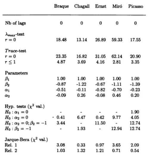
Table A3 Cointegration between individual artists (ReI. 1) and the global market (ReI. 2)

Braque Chagall Ernst Miró Picasso

Nb of lags O O O O O Àmax-test r=O 18.48 13.14 26.89 59.33 17.55 Trace-test r=O 23.35 16.82 31.05 62.14 20.90 r ~ 1 4.87 3.69 4.16 2.81 3.35 Parameters f31 1.00 1.00 1.00 1.00 1.00 f32 -0.87 -1.22 -0.67 -1.11 -1.39 01 -0.51 -0.11 -0.82 -0.70 -0.23 02 -0.09 0.26 -0.08 0.46 0.20

Hyp. tests (X2 val.)

Ho: 01 = O 1.90 Ho: 02 =0 • 0.41 6.47 0.42 9.77 4.05 Ho : 02 = O; f32 = -1 3.44 11.50 12.74 Ho : f32 = -1 1.93 12.94 12.74 Jarque-Bera (X2 val.) ReI. 1 3.08 0.33 0.97 3.65 2.09 ReI. 2 1.03 1.32 1.21 0.71 0.54

The criticai values at the 5% probability levei are:

14.04 for the Àmoz-test and 15.20 and 3.96 for the Trace-test.

3.84 and 5.99 for the :e-test with 1 and 2 d.f. 5.99 for the Jarque-Bera test (X2 with 2 d.f.).

(24)

I

i i

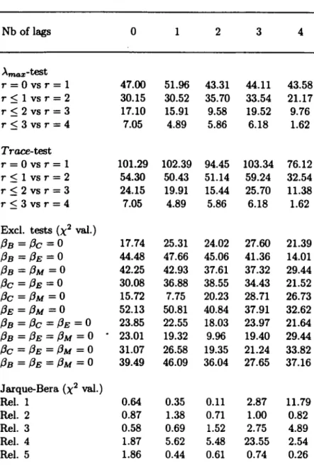
Table A4 Cointegration between the tive individual artists and exclusion tests for two and three artists

Nb of lags O 1 2 3 4 Àmaz-test r=Ovsr=l 47.00 51.96 43.31 44.11 43.58 r:$lvsr=2 30.15 30.52 35.70 33.54 21.17 r:$2vsr=3 17.10 15.91 9.58 19.52 9.76 r:$3vsr=4 7.05 4.89 5.86 6.18 1.62 Trace-test r=Ovsr=l 101.29 102.39 94.45 103.34 76.12 r:$lvsr=2 54.30 50.43 51.14 59.24 32.54 r:$2vsr=3 24.15 19.91 15.44 25.70 11.38 r:$3vsr=4 7.05 4.89 5.86 6.18 1.62

ExcI. tests (X 2 val.)

13B

=

13c

= O 17.74 25.31 24.02 27.60 21.39

13B

=

13E

= O 44.48 47.66 45.06 41.36 14.01

13B

=

13M

= O 42.25 42.93 37.61 37.32 29.44

13c

=

13E

= O 30.08 36.88 38.55 34.43 21.52

13c

=

13M

= O 15.72 7.75 20.23 28.71 26.73

13E

=

13M

= O 52.13 50.81 40.84 37.91 32.62

13B

=

13c

=

13E

= O 23.85 22.55 18.03 23.97 21.64

13B

=

13E

=

13M

= O

.

23.01 19.32 9.96 19.40 29.44

13c

=

13E

=

13M

= O 31.07 26.58 19.35 21.24 33.82

13B

=

13E

=

13M

= O 39.49 46.09 36.04 27.65 37.16 Jarque-Bera (X2 val.) ReI. 1 0.64 0.35 0.11 2.87 11.79 ReI. 2 0.87 1.38 0.71 1.00 0.82 ReI. 3 0.58 0.69 1.52 2.75 4.89 ReI. 4 1.87 5.62 5.48 23.55 2.54 ReI. 5 1.86 0.44 0.61 0.74 0.26

The criticaI values at the 5% probability leveI are: 27.17,20.78,14.04 and 3.96 for the À"'G",-test 47.18, 29.51, 15.20 and 3.96 for the Trace-test. 5.99, 7.81 and 9.49 for the :e-test with 2, 3 and 4 d.f. 5.99 for the Jarque-Bera test (X2 _{with 2 dJ.).}

(25)

- - - -- ~---- _ .

-Table A5 Cointegration between the five individual artists Model coefficients (K = 1

Relation Oil Oi2 'riB,1 'riC.I 'riE,1 'riM, I riP,1 Ho : 'riC,1 =

'riM,1

=

O Braque -0.33 -0.49 -0.02 -0.19 -0.23 0.02 0.01 (-0.15) (-1.06) (-1.86) (0.17) (0.10) 0.54 Chagall -0.17 0.06 0.07 -0.58 0.05 0.26 -0.02 (0.06) (-4.29) (0.55) (2.67) (-1.79) 9.93 Ernst 1.02 -0.08 -0.11 0.10 -0.12 0.23 0.02 (-0.52) (0.43) (-0.69) (1.30) (0.15) 1.30 Miró 0.05 -0.26 -0.15 -0.32 0.08 0.16 0.11 (-0.85) (-1.47) (0.54) (-1.04) (0.80) 2.49 Picasso 0.00 0.00 -0.41 0.11 0.03 0.40 -0.36 (-) (-) (-2:66) (0.48) (0.22) (2.52) ( -2.52) 4.19

t-statistics are given between brackets, under the coefficients.

The statistic in the last column is ao F-variable with 2 aod 45 d.r. Its criticai value at 5% is 3.21.

(26)

A

Et'ISAtOS ECOt'IOJ'/UCOS

OJ.\

EPGE

200. A VISÃO TEÓRICA SOBRE MODELOS PREVIDENCIÁRIOS: O CASO BRASILEIRO

-Luiz Guilhenne Schymura de Oliveira - Outubro de 1992 - 23 pág. (esgotado)

201. HIPERINFLAÇÃO: CÂMBIO, MOEDA E ÂNCORAS NOMINAIS - Fernando de Holanda

Barbosa - Novembro de 1992 - 10 pág. (esgotado)

202. PREVIDÊNCIA SOCIAL: CIDADANIA E PROVISÃO - Clovis de Faro - Novembro de

1992 - 31 pág. (esgotado)

203. OS BANCOS ESTADUAIS E O DESCONTROLE FISCAL: ALGUNS ASPECTOS

-Sérgio Ribeiro da Costa Werlang e Annínio Fraga Neto - Novembro de 1992 - 24 pág.

(esgotado)

204. TEORIAS ECONÔMICAS: A MEIA-VERDADE TEMPORÁRIA - Antonio Maria da

Silveira - Dezembro de 1992 - 36 pág. ( esgotado)

205. THE RICARDIAN VICE AND THE INDETERMINA TION OF SENIOR - Antonio Maria

da Silveira - Dezembro de 1992 - 35 pág. (esgotado)

206. HIPERINFLAÇÃO E A FORMA FUNCIONAL DA EQUAÇÃO DE DEMANDA DE

MOEDA - Fernando de Holanda Barbosa - Janeiro de 1993 - 27 pág. (esgotado)

207. REFORMA FINANCEIRA - ASPECTOS GERAIS E ANÁLISE DO PROJETO DA LEI

COMPLEMENTAR - Rubens Penha Cysne - fevereiro de 1993 - 37 pág. (esgotado)

208. ABUSO ECONÔMICO E O CASO DA LEI 8.002 - Luiz Guilhenne Schymura de Oliveira e

Sérgio Ribeiro da Costa Werlang - fevereiro de 1993 - 18 pág. (esgotado)

209. ELEMENTOS DE UMA ESTRATÉGIA PARA O DESENVOLVIMENTO DA

AGRICULTURA BRASILEIRA Antonio Salazar Pessoa Brandão e Eliseu Alves

-Fevereiro de 1993 - 370pág.

210. PREVIDÊNCIA SOCIAL PÚBLICA: A EXPERIÊNCIA BRASILEIRA -

Hélio

Portocarrero de Castro, Luiz Guilhenne Schymura de Oliveira, Renato Fragelli Cardoso e

Uriel de Magalhães - Março de 1993 - 35 pág - (esgotado).

211. OS SISTEMAS PREVIDENCIÁRIOS E UMA PROPOSTA PARA A REFORMULACAO

DO MODELO BRASILEIRO - Helio Portocarrero de Castro, Luiz Guilhenne Schymura de

Oliveira, Renato Fragelli Cardoso e UrieI de Magalhães Março de 1993 43 pág.

-(esgotado)

212. THE INDETERMINATION OF SENIOR (OR THE INDETERMINATION OF WAGNER)

AND SCHMOLLER AS A SOCIAL ECONOMIST - Antonio Maria da Silveira - Março de

1993 - 29 pág. (esgotado)

213. NASH EQUILIBRIUM UNDER KNIGHTIAN UNCERTAINTY: BREAKING DOWN

BACKWARD INDUCTION (ExtensiveIy Revised Version) - James Dow e Sérgio Ribeiro

da Costa Werlang - Abril de 1993 36 pág.

214. ON THE DIFFERENTIABILITY OF THE CONSUMER DEMAND FUNCTION - Paulo

(27)

-215.

DETERMINAÇÃO DE PREÇOS DE ATIVOS, ARBITRAGEM, MERCADO A TERMO E

MERCADO FUTURO Sérgio Ribeiro da Costa Werlang e Flávio Auler Agosto de 1993

-69 pág. (esgotado).

216. SISTEMA MONETÁRIO VERSÃO REVISADA - Mario Henrique Simonsen e Rubens

Penha Cysne - Agosto de 1993 - 69 pág. (esgotado).

217. CAIXAS DE CONVERSÃO - Fernando Antônio Hadba - Agosto de 1993 - 28 pág.

218. A ECONOMIA BRASILEIRA NO PERÍODO MILITAR - Rubens Penha Cysne - Agosto de

1993 - 50 pág. (esgotado).

219. IMPÔSTO INFLACIONÁRIO E TRANSFERÊNCIAS INFLACIONÁRIAS

-

Rubens

Penha Cysne - Agosto de 1993 - 14 pág. (esgotado).

220. PREVISÕES DE Ml COM DADOS MENSAIS Rubens Penha Cysne e João Victor Issler

-Setembro de 1993 - 20 pág.

221. TOPOLOGIA E CÁLCULO NO

Rn -

Rubens Penha Cysne e Humberto Moreira

-Setembro de 1993 - 106 pág. (esgotado)

222. EMPRÉSTIMOS DE MÉDIO E LONGO PRAZOS E INFLAÇÃO: A QUESTÃO DA

INDEXAÇÃO - Clovis de Faro - Outubro de 1993 - 23 pág.

223. ESTUDOS SOBRE A INDETERMINAÇÃO DE SENIOR, vol. 1 - Nelson H. Barbosa,

Fábio N.P. Freitas, Carlos F.L.R. Lopes, Marcos B. Monteiro, Antonio Maria da Silveira

(Coordenador) e Matias Vemengo - Outubro de 1993 - 249 pág (esgotado)

224. A SUBSTITUIÇÃO DE MOEDA NO BRASIL: A MOEDA INDEXADA - Fernando de

Holanda Barbosa e Pedro Luiz Valls Pereira - Novembro de 1993 - 23 pág.

225. FINANCIAL INTEGRA TION AND PUBLIC FINANCIAL INSTITUTIONS - Walter

Novaes e Sérgio Ribeiro da Costa Werlang - Novembro de 1993 - 29 pág

226. LA WS OF LARGE NUMBERS FOR NON-ADDITIVE PROBABILITIES - James Dow e

Sérgio Ribeiro da Costa Werlang - Dezembro de 1993 - 26 pág.

227. A ECONOMIA BRASILEIRA NO PERÍODO MILITAR - VERSÃO REVISADA - Rubens

Penha Cysne - Janeiro de 1994 - 45 pág. (esgotado)

228. THE IMP ACT OF PUBLIC CAPITAL AND PUBLIC INVESTMENT ON ECONOMIC

GROWTH: AN EMPIRICAL INVESTIGA TION - Pedro Cavalcanti Ferreira - Fevereiro de

1994 - 37 pág. (esgotado)

229. FROM

THE

BRAZILIAN

PAY

AS

VOU

GO

PENSION

SYSTEM

TO

CAPITALIZATION: BAILING OUT THE GOVERNMENT - José Luiz de Carvalho e

Clóvis de Faro - Fevereiro de 1994 - 24 pág.

230. ESTUDOS SOBRE A INDETERMINAÇÃO DE SENIOR - vol. 11 - Brena Paula Magno

Fernandez, Maria Tereza Garcia Duarte, Sergio Grumbach, Antonio Maria da Silveira

(Coordenador) - Fevereiro de 1994 - 51 pág.(esgotado)

231. ESTABILIZAÇÃO DE PREÇOS AGRÍCOLAS NO BRASIL: AVALIAÇÃO E

PERSPECTIV AS - Clovis de Faro e José Luiz Carvalho - Março de 1994 - 33 pág.

(esgotado)

232. ESTIMA TING SECTORAL CYCLES USING COINTEGRA TION AND COMMON

FEA TURES - Robert F. Engle e João Victor Issler - Março de 1994 - 55 pág

(28)

233. COMMON CYCLES IN MACROECONOMIC AGGREGATES - João Victor Issler e Farshid Vahid - Abril de 1994 - 60 pág.

234. BANDAS DE CÂMBIO: TEORIA, EVIDÊNCIA EMPÍRICA E SUA POSSÍVEL APLICAÇÃO NO BRASIL - Aloisio Pessoa de Araújo e Cypriano Lopes Feijó Filho - Abril de 1994 - 98 pág. (esgotado)

235. O HEDGE DA DÍVIDA EXTERNA BRASILEIRA - Aloisio Pessoa de Araújo, Túlio Luz Barbosa, Amélia de Fátima F. Semblano e Maria Haydée Morales - Abril de 1994 - 109 pág. (esgotado)

236. TESTING THE EXTERNALITIES HYPOTHESIS OF ENDOGENOUS GROWTH USING

COINTEGRA TION - Pedro Cavalcanti Ferreira e João Victor Issler - Abril de 1994 - 37 pág. (esgotado)

237. THE BRAZILIAN SOCIAL SECURITY PROGRAM: DIAGNOSIS AND PROPOSAL FOR REFORM - Renato Fragelli; Uriel de Magalhães; Helio Portocarrero e Luiz Guilherme Schymura - Maio de 1994 - 32 pág.

238. REGIMES COMPLEMENTARES DE PREVIDÊNCIA - Hélio de Oliveira Portocarrero de Castro, Luiz Guilherme Schymura de Oliveira, Renato Fragelli Cardoso, Sérgio Ribeiro da Costa Werlang e Uriel de Magalhães - Maio de 1994 - 106 pág.

239. PUBLIC EXPENDITURES, TAXATION AND WELFARE MEASUREMENT - Pedro Cavalcanti Ferreira - Maio de 1994 - 36 pág.

240. A NOTE ON POLICY, THE COMPOSITION OF PUBLIC EXPENDITURES AND ECONOMIC GROWTH - Pedro Cavalcanti Ferreira - Maio de 1994 - 40 pág.

241. INFLAÇÃO E O PLANO FHC - Rubens Penha Cysne - Maio de 1994 - 26 pág. (esgotado) 242. INFLATIONARY BIAS AND STATE OWNED FINANCIAL INSTITUTIONS - Walter

Novaes Filho e Sérgio Ribeiro da Costa Werlang - Junho de 1994 -35 pág.

243. INTRODUÇÃO À INTEGRAÇÃO ESTOCÁSTICA - Paulo Klinger Monteiro - Junho de 1994 - 38 pág. (esgotado)

244. PURE ECONOMIC THEORIES: THE TEMPORARY HALF-TRUTH - Antonio M. Silveira - Junho de 1994 - 23 pág. (esgotado)

245. WELFARE COSTS OF INFLATION - THE CASE FOR INTEREST-BEARING MONEY AND EMPIRICAL ESTIMA TES FOR BRAZIL - Mario Henrique Simonsen e Rubens Penha Cysne - Julho de 1994 - 25 pág. (esgotado)

246. INFRAESTRUTURA PÚBLICA, PRODUTIVIDADE E CRESCIMENTO - Pedro Cavalcanti Ferreira - Setembro de 1994 - 25 pág.

247. MACROECONOMIC POLICY AND CREDIBILITY: A COMPARATIVE STUDY OF THE FACTORS AFFECTING BRAZILIAN AND ITALIAN INFLATION AFTER 1970-Giuseppe Tullio e Marcio Ronci - Outubro de 1994 - 61 pág. (esgotado)

248. INFLATION AND DEBT INDEXATION: THE EQUIVALENCE OF TWO

ALTERNA TIVE SCHEMES FOR THE CASE OF PERIODIC PA YMENTS - Clovis de Faro - Outubro de 1994 -18 pág.

(29)

-~.-

-249. CUSTOS DE BEM ESTAR DA INFLAÇÃO - O CASO COM MOEDA INDEXADA E

ESTIMA TIV AS EMPÍRICAS PARA O BRASIL - Mario Henrique Simonsen e Rubens Penha Cysne - Novembro de 1994 - 28 pág. (esgotado)

250. THE ECONOMIST MACHIA VELLI Brena P. M. Femandez e Antonio M. Silveira -Novembro de 1994 - 15 pág.

251. INFRAESTRUTURA NO BRASIL: ALGUNS FATOS ESTILIZADOS - Pedro Cavalcanti Ferreira - Dezembro de 1994 - 33 pág.

252. ENTREPRENEURIAL RISK AND LABOUR'S SHARE IN OUTPUT - Renato Fragelli Cardoso - Janeiro de 1995 - 22 pág.

253. TRADE OR INVESTMENT

?

LOCA TION DECISIONS UNDER REGIONAL

INTEGRATION - Marco Antonio F.de H. Cavalcanti e Renato G. Flôres Jr. - Janeiro de 1995 - 35 pág.

254. O SISTEMA FINANCEIRO OFICIAL E A QUEDA DAS TRANFERÊNCIAS INFLACIONÁRIAS - Rubens Penha Cysne - Janeiro de 1995 - 32 pág.

255. CONVERGÊNCIA ENTRE A RENDA PERCAPITA DOS ESTADOS BRASILEIROS -Roberto G. Ellery Jr. e Pedro Cavalcanti G. Ferreira - Janeiro 1995 - 42 pág.

256. A COMMENT ON liRA TIONAL LEARNING LEAD TO NAS H EQUILIBRIUM" BY PROFESSORS EHUD KALAI EHUD EHUR - Alvaro Sandroni e Sergio Ribeiro da Costa Werlang - Fevereiro de 1995 - 10 pág.

257. COMMON CYCLES IN MACROECONOMIC AGGREGATES (revised version) - João Victor Issler e Farshid Vahid - Fevereiro de 1995 - 57 pág.

258. GROWTH, INCREASING RETURNS, AND PUBLIC INFRASTRUCTURE: TIMES SERIES EVIDENCE (revised version) Pedro Cavalcanti Ferreira e João Victor Issler -Março de 1995 - 39 pág.( esgotado)

259. POLÍTICA CAMBIAL E O SALDO EM CONTA CORRENTE DO BALANÇO DE PAGAMENTOS -

Anais do Seminário realizado na Fundação Getulio Vargas no dia 08 de

dezembro de

1994 - Rubens Penha Cysne (editor) - Março de 1995 - 47 pág. (esgotado) 260. ASPECTOS MACROECONÔMICOS DA ENTRADA DE CAPITAIS -

Anais do Seminário

realizado na Fundação Getulio Vargas no dia 08 de dezembro de

1994 - Rubens Penha Cysne (editor) - Março de 1995 - 48 pág. (esgotado)

261. DIFICULDADES DO SISTEMA BANCÁRIO COM AS RESTRIÇÕES ATUAIS E COMPULSÓRIOS ELEVADOS -

Anais do Seminário realizado na Fundação Getulio

Vargas no dia 09 de dezembro de

1994 Rubens Penha Cysne (editor) Março de 1995 -47 pág. (esgotado)

262. POLÍTICA MONETÁRIA: A TRANSIÇÃO DO MODELO ATUAL PARA O MODELO CLÁSSICO -