Sónia Daniela Paredes Rodrigues
abril de 2017
Do cash holdings protect firms from
a takeover bid?
Sónia Daniela P
ar
edes Rodrigues
Do cash holdings pro
tect firms from a t
ak
eo
ver bid?
UMinho|20
Sónia Daniela Paredes Rodrigues
Do cash holdings protect firms from
a takeover bid?
Trabalho efetuado sob a orientação do
Professor Doutor Gilberto Ramos Loureiro
Dissertação de Mestrado
Acknowledgments
I would like to express my deep gratitude to my supervisor, Professor Gilberto Loureiro, for accepting to be my supervisor, the constant support and the constructive comments. I also want to thank Professor João Paulo Silva for his insightful comments and suggestions about my English, which increased the quality of my dissertation. Last but not least, I am grateful to my family and friends, especially Ricardo Ferreira, for all the encouragement and support throughout my dissertation.
Do cash holdings protect firms from a takeover bid?
Abstract
In my research, I study the relationship between a firm’s cash holdings and its probability of being acquired. The sample consists of 428 Euro zone targets, of which 13 are hostile targets, between 2000 and 2015 and includes a control sample that were not targets of acquisitions during the period. In the literature the conventional wisdom states that firms with more cash holdings are more likely to be targets of mergers & acquisitions (M&A) because they are more liquid and attractive to potential buyers. Alternatively, Pinkowitz (2002) finds the opposite result and argues that, due to agency costs of excessive cash, cash-rich firms are less likely to be acquired. In support of this view, and contradicting the conventional wisdom, I find, for the group of firms with poor growth opportunities, evidence that higher levels of cash holdings decreases the likelihood of being targets. However, in the overall sample, this result is not robust as I only find some marginal evidence to support this view. In contrast, using the overall sample, I do find that higher levels of negative excess cash reduce the probability of being a target. I also find that firms with less cash holdings are exposed to a higher probability of an acquisition being successful. In addition, I test whether targets firms with high cash holdings are more likely to have higher bid premiums, which I find to be an accurate statement, supporting Stulz’s (1988) research.
As reservas de caixa protegem as empresas de uma oferta pública de aquisição? Resumo
O presente estudo teve como propósito avaliar a relação entre as reservas de caixa que uma empresa detém e a sua probabilidade de ser adquirida. Para isso, utilizo uma amostra constituída por 428 empresas da zona Euro que foram alvo de propostas de aquisição, entre 2000 e 2015, das quais 13 foram alvo de aquisições hostis, e incluo também uma amostra de controlo. Recorrendo à literatura, a maioria dos autores afirma que as empresas com mais reservas em caixa estão mais propensas a serem alvo de fusões e aquisições, porque são mais líquidas e atrativas para potenciais compradores. Por outro lado, Pinkowitz (2002) defende o oposto, argumentando que, devido aos custos de agência resultantes de excessivas reservas de caixa, as empresas ricas em reservas de caixa são menos suscetíveis de serem adquiridas. Os resultados deste estudo demonstram que, para o grupo de empresas com menores oportunidades de crescimento, elevados níveis de caixa reduzem a probabilidade de serem adquiridas. Contudo, considerando a amostra total, este resultado não é robusto, sendo apenas marginalmente significativo. Contrariamente, usando a amostra total, os resultados sugerem que elevados défices de caixa reduzem a probabilidade de uma empresa ser adquirida. Para além disso, é possível concluir que as empresas com menores reservas de caixa estão expostas a uma maior probabilidade de uma aquisição se concretizar. Adicionalmente, as empresas que têm mais reservas de caixa têm tendência a receber prémios de oferta mais elevados, tal como defende Stulz (1988). De uma forma geral, com este estudo concluo que existe uma relação direta entre o dinheiro em caixa e a probabilidade da empresa ser adquirida, bem como com os prémios de oferta.
Palavras-chave: dinheiro em caixa, alvos de fusões e aquisições, probabilidade de aquisição, prémio de oferta
Table of Contents Acknowledgments ... iii Abstract ... v Resumo ... vii Table of Contents ... ix List of Tables ... xi 1. Introduction ... 1 2. Literature Review ... 2
2.1. Likelihood of becoming a takeover target ... 4
2.2. Bid Premium ... 6
3. Methodology ... 8
4. Data ... 11
5. Results ... 17
5.1. Probability of an acquisition ... 17
5.2. Probability of being targeted ... 24
5.3. Robustness test ... 28
5.4. Probability of completion ... 28
5.5. Bid premium ... 30
6. Hostile targets ... 33
6.1. Probability of an acquisition ... 33
6.2. Probability of being targeted ... 34
7. Conclusion ... 35
References ... 37
Appendix A – Description of the variables ... 42
List of Tables
Table 1 – Description of the targets by country ... 12
Table 2 – Summary statistics ... 13
Table 3 – Correlation table ... 16
Table 4 – Probit regression for the likelihood of being acquired ... 18
Table 5 – Probit regression in determining the likelihood of being acquired for firms with poor investment opportunities ... 20
Table 6 – Probit regression determining the likelihood of being acquired and gaining control .... 22
Table 7 – Probit regression determining the likelihood of being targeted ... 24
Table 8 – Probit regression determining the likelihood of being targeted for firms with poor investment opportunities ... 26
Table 9 – Probit regression determining the likelihood of completion ... 29
1. Introduction
In this study, I analyse the relationship between a firm’s cash holdings and its probability of being acquired. The aim of my research is to understand whether firms use their levels of cash holdings to affect the outcome of potential takeovers. The conventional wisdom states that firms with more cash holdings are more likely to be targets of mergers & acquisitions (M&A) because they are more liquid and attractive to potential buyers. Thus, managers who want to prevent their companies from being acquired should reduce their levels of cash holdings. Jensen (1986) uses this argument to conclude that the market for corporate control monitors the levels of firms’ cash holdings. Alternatively, Pinkowitz (2002) finds the opposite result – firms with more cash holdings are less likely to be acquired. In fact, excessive cash holdings raise concerns about agency costs and increase the likelihood of expropriation of minority shareholders. Moreover, these firms may even be more difficult to value as managers can easily cash out liquid assets to pay their shareholders. Therefore, cash holdings may have the effect of repelling potential acquirers.
In this study, I examine the European market, more specifically the Euro zone, for corporate control and test alternative explanations. My sample consists of 428 targets, of which 13 are hostile targets of acquisitions occurred between 2000 and 2015, and a control sample of firms that were not targets of acquisitions in this period. In addition to studying the effect of excessive cash holdings on the likelihood of being a target, I also test whether excessive cash holdings affect the acquisition bid premium. For this analysis, I include the control factor to test its effect on the bid premium.
In order to test my hypotheses and reinforce my results, I use different sub-analyses and a robustness test. The sub-analyses consist in restricting the sample in different ways, such as firms with poor investment opportunities, successful targets and successful targets where the acquirer got more than 50% control of the target. In the robustness test I perform the same analysis using a sample of matched firms by year and size. Apart from examining the probability of a cash rich firm being targeted or acquired, I use another probabilistic regression to examine the marginal effect of a targeted firm effectively being acquired. In other words, I test the probability of completion of a takeover attempt.
As I draw on the Pinkowitz (2002) study and he uses hostile targets, I do an additional analysis of my hypothesis using just the hostile targets. Although I have a reduced number of hostile targets, I compare the results in order to see whether there are any differences between a friendly and a hostile target.
The next main sections of my dissertation include the literature review in section 2 explaining my three main hypotheses, the methodology in section 3, a short description of the data in section 4, and the results in section 5. Section 6 shows the results for the hostile targets and in the last section 7, I present my conclusions.
2. Literature Review
The literature provides several possible determinants which explain why firms may retain excess cash and its possible influence on the probability of a firm being a target of a takeover bid. Couderc (2005) investigates the determinants of cash holdings and their consequences on the firms’ profitability from 1989 to 2002 in Canada, France, Germany, Great-Britain and the USA. The author finds a positive relationship between corporate cash holdings and firm size, cash flow level and cash flow variability. Opler, Pinkowitz, Stulz & Williamson (1999) and Pinkowitz & Williamson (2007) find that firms with strong growth opportunities and firms with riskier activities hold more cash than other firms. In addition, Opler, Pinkowitz, Stulz & Williamson (1999) explain that firms that have greater access to capital markets tend to hold less cash, which avoids costs for external funding. At the same time, the easier access to capital markets allows the firm to increase its cash holdings whenever it is needed, for example to avoid being targeted. Additionally, Faulkender & Wang (2006) show through an event study that the value of cash is higher when there are low levels of cash holdings, low leverage and constraints in accessing financial markets. Moreover, Ferreira & Vilela (2004) also investigate the determinants of cash balances but for firms in EMU countries from the years 1987 to 2000. In this paper, they show that cash holdings have a positive relationship with investment opportunities, but a negative relationship with the value of liquid assets and leverage. Furthermore, they provide evidence of a significant negative relationship between bank debt and cash holdings. Ali & Yousaf (2013) examine the determinants of cash holdings in non-financial firms by taking a sample of 876 German firms between the years 2000 to 2010. They find that cash holdings are negatively correlated with the size of the firm, market-to-book value and leverage, in line with the existing literature. Furthermore, Bates, Kahle & Stulz (2009) document the dramatic increase in the average cash ratio for US firms from 1980 to 2006. They find that the cash ratio increases due to a fall in inventories and capital expenditures and an increase in cash flow risk and R&D expenditures.
Dittmar & Mahrt-Smith (2007) show that entrenched managers are more likely to build excess cash balances. They provide evidence that cash is less valuable when agency problems between shareholders are greater, which is consistent with the findings of Pinkowitz, Stulz & Williamson (2006). The agency problems lead to agency costs and dissatisfaction of the shareholders, which can benefit a hostile takeover.
In order to examine if the style of corporate governance influences the firm’s decision to liquidate assets, Anderson & Hamadi (2006) use a panel data set of Belgian firms. They show strong risk aversion by family firms, which leads to higher cash holdings. La Porta, Lopez-de-Silanes & Shleifer (1999) add that in countries with poor shareholder protection even the largest firms tend to have controlling shareholders. In addition, La Porta, Lopez-de-Silanes, Shleifer & Vishny (1998) analyse the investor protection laws and the quality of their enforcement in 49 countries. They conclude that the Common-Law countries tend to protect investors more than the Civil-Law countries, especially the French speaking Civil-Law countries, and that the law enforcement is also stronger in Common-Law countries than in French- speaking Civil-Law countries. Low protection of shareholders and controlling shareholders make it easier for managers to cash out liquid assets whenever there is a takeover threat.
However, Han & Qiu (2007) test publicly traded firms from 1997 to 2002 and show empirically that there is a significantly positive relationship between cash flow volatility and cash holdings in financially constrained firms. On the other hand, they show that the same relationship is not significant in financially unconstrained firms, which is consistent with the empirical findings from Almeida, Campello & Weisbach (2004).In other words, the more cash volatility a firm has, the more cash it holds in order to overcome unexpected losses and avoid excessive costs for external fund raising.
Furthermore, previous literature shows that there is an impact of investors’ preferences on cash holdings’ policies. Baker & Wurgler (2004) and Breuer, Rieger & Soypak (2016) provide evidence that companies adjust dividend payouts, while Baker Greenwood & Wurgler (2009) find that they adjust mergers and acquisitions according to investors’ preferences.
Overall, all the previous mentioned determinants are predicted by the pecking order and the trade-off theories. These two theories play an important role in explaining the determinants of firms’ cash holdings and their benefits. Excessive cash holdings do not only reduce the likelihood of financial distress and provide flexibility, but they also decrease information asymmetries. Moreover,
they reduce agency costs, provide safety reserves to prepare for unexpected losses and avoid excessive costs for external fund raising. According to Pinkowitz (2002, p. 36), “firms boost their cash when takeover probability increases”. Therefore, the previous mentioned determinants of cash holdings may serve to increase the firm’s cash amount and prevent them from a takeover bid.
2.1. Likelihood of becoming a takeover target
The conventional wisdom states that firms with large cash holdings are more likely to become takeover targets. Jensen (1986) is one of the authors that argues that firms with free cash flow that refuse to pay out to shareholders are more likely to become takeover targets. Therefore, the author argues that the market for corporate control can monitor cash holdings of firms. Dittmar, Mahrt-Smith & Servaes (2003) use a sample of more than 11, 000 firms from 45 countries and find that firms from countries with low shareholder protection hold twice as much cash as their peers from countries with high shareholder protection. La Porta, Lopez-de-Silanes, Shleifer & Vishny (2000) also find that countries with better protection of minority shareholders pay higher dividends, which may cause shareholders to start a proxy fight to trigger a potential acquisition to replace the current manager. According to Faleye (2004), firms which are proxy fight targets hold 23% more cash than non-targets, which supports the conventional wisdom. In addition, Gao (2015) finds that targets hold more cash to attract acquirers since it can reduce future acquisitions costs.
However, there are many authors contradicting the conventional wisdom. Harford (1999) finds that cash rich firms are more likely to attempt acquisitions and, therefore, are less likely to be takeover targets. High cash holdings provide flexibility to the firm and enable it to defend itself from takeover bids. A way to prevent being a target is to pay out the excess cash to the shareholders or repurchase its stocks from the market. Dann & DeAngelo (1988) find that stock repurchase prevents firms from being acquired. The more stocks outstanding, the less ownership control the management has. Also, Stulz (1988) and Harris & Raviv (1988) argue that a way to hamper an acquisition is to use its cash holdings to repurchase stocks in order to increase the ownership control of the firm.
Pinkowitz (2002) investigates whether the market for corporate control monitors cash holdings. Using hostile takeover attempts, Pinkowitz analyses the impact of cash on acquisition probability and concludes that cash holdings do not make a firm more likely to be acquired. The author
extended his research by examining cash holdings when antitakeover laws are enacted and cash holdings of non-target firms in industries where hostile takeovers occur. He concludes that firms hold significantly less cash once the law is effective and that the takeover market does not monitor cash holdings. Moreover, Schauten, van Dijk & van der Waal (2013) use different European firms to show the positive relationship between the value of excess cash and the takeover defences governance score. They observe this positive relationship especially for firms from Common-Law countries, namely the UK and Ireland, rather than for firms from Civil-Law countries, which in this case were Germany and Scandinavian countries. This means that the excess cash of these firms has a lower value due to the insufficient supervision of the law. Another author who shows evidence against the conventional wisdom is Gao (2015). He builds an infinite-horizon dynamic model to investigate the relationship between corporate takeovers and cash holdings. The author finds a positive relationship between acquisition opportunities and cash reserves, justifying that acquirers hold more cash because they have larger incentives to reduce external financing costs.
Pinkowitz & Williamson (2001) examine the relationship between bank debt and cash holdings and the effect of bank power on the cash holdings of industrial firms from USA, Germany and Japan. They find a positive relationship between bank debt and cash holdings and, also, that countries with high bank power have higher levels of cash, which is the case of Japan. But there is also research that proves that several firm and industry-specific variables, such as firm size, liquidity and growing opportunity, influence the takeover probability, as is the case of Powell & Thomas (1994). In addition, Ambrose & Megginson (1992) find that the probability of receiving a takeover bid is positively related with tangible assets and negatively related with firm size and to the net changes in institutional holdings.
With the purpose of applying Pinkowitz’s (2002) study to the European market, I formulate the following main testable hypotheses:
H1A: Firms with higher levels of cash holdings are less likely to be targets in a takeover bid. H1B: Firms with poor investment opportunities and higher levels of cash holdings are less likely
to be targets in a takeover bid.
For the hypothesis H1A I do several sub-analyses in order to reinforce my results. The aim of the hypothesis H1B is to restrict my sample by using the targets with poor investment opportunity
and to analyse whether the poor investment opportunities do have any influence on the takeover probability. An environment of poor investment opportunity can lead to a poor performance of a firm. According to Palepu (1986) there is a negative relationship between the probability of takeover and the poor performance of a firm. On the other hand, Franks & Mayer (1996) conclude the opposite in their study for the UK market.
Pinkowitz’s (2002) study tests just hostile takeovers and finds no evidence of a positive relationship between cash holdings and its probability of being acquired. A hostile takeover is defined as more aggressive than a friendly takeover, since the acquirer tries to overcome the company's board of director by gaining control or persuading existing shareholders. However, even the friendly and hostile takeovers can be distinguished, Schwert (2000) finds no evidence in economic terms, which means that there should not exist any differences in the results of my study using all targets and not just hostile targets.
In addition, in order to test whether the cash holdings protect firms from being successfully acquired once it is already a takeover target, I formulate the following testable hypothesis:
H2: Firms with higher levels of cash holdings are less likely to be successfully acquired once it is a target in a takeover bid.
According to Pinkowitz (2002), the excess cash holdings do avoid an acquisition being successfully completed. In other words, once a firm is targeted, the acquisition can be avoided by boosting their cash holdings.
2.2. Bid Premium
The literature provides several possible factors which affect the bid premium. Dimopoulos & Sacchetto (2014) find that the magnitude of the bid premium is related with the target resistance. The higher the resistance of the target, the higher the bid premium. Also, Fishman (1989) finds that cash holdings are negatively related with the target resistance. The larger the cash holdings, the lower the target resistance. This hypothesis is supported by Pinkowitz’s (2002) argument that excessive cash holdings make firms less attractive as targets. Another determinant of a higher bid premium is the cost that the bidder is willing to pay in order to deter other rival bidders, according to Fishman (1988) and Jennings & Mazzeo (1993). Bris (2002) shows that the bidder must pay a cost in order to gain control. In addition, the author studies the strategies that the bidder should
consider depending on the size of the toehold. There are other determinants that influence the bid premium. For example, Bargeron’s (2012) sample includes tender offers from 1995 to 2010, where more than half contain a Shareholder Tender Agreement1, and finds that they are related with lower premiums. Moreover, Flanagan & O’Shaughnessy (2003) conclude from their research that the bid premium depends on whether the bidder’s core business is related to the target. If various bidders are competing for the same target, the bidder with a related core business will offer a lower premium. Eckbo (2009) argues that the bid premium is higher when the offer is made in cash rather than in stocks.
On the one hand, Bange & Mazzeo (2004) find that a high bid premium is related to the characteristics of the target board. In other words, the firm will require a higher bid premium in order to compensate the personal losses from the takeover. Chatterjee, John & Yan (2012) show that the higher the divergence of investors’ opinion, the higher the bid premium is. But, in general, the bidder offers a positive bid premium because the beliefs about the value of the target is similar. On the other hand, according to Betton & Eckbo (2000), Walkling (1985), Betton, Eckbo & Thorburn (2009) the toehold of the bidder is positively related to the probability of successfully acquiring a target. For instance, Betton, Eckbo & Thorburn (2009) use a sample of over 10,000 U.S. public targets and show that the higher the bidder’s toehold on the target company before the acquisition is, the higher the probability of completing the acquisition and gaining control of the target is.
If the bidder holds a high toehold, it facilitates acquiring information about the target and thereby gaining advantage over its rival competitors. According to Jennings & Mazzeo (1993, p. 907), “situations in which information about the target appears to be plentiful are associated with greater likelihoods of resistance and competition.” Betton & Eckbo (2000) add in their conclusions that the toehold is negatively related with the bid premium, indicating that the toehold has a deterrent effect. In other words, the higher the toehold, the lower the bid premium, because the toehold provides power to the acquirer and, therefore, there will be no need to offer a high bid premium for the target.
Considering what the literature states about the bid premium, I formulate a third testable hypothesis:
H3: Target firms with higher levels of cash holdings are more likely to have higher bid premiums.
For this hypothesis, I also perform several sub-analyses in order to reinforce my results. Therefore, I also test the hypothesis by restricting my sample and using just the targets with poor investment opportunity. The aim of this hypothesis is to test if my sample supports the argument of Stulz (1988), who finds a positive relationship between cash and bid premium.
3. Methodology
In order to test my main hypothesis, I first have to define the variable Excess Cash. As Pinkowitz (2002) does in his research, I use the following OLS regression:
(1) 𝐸𝑥𝑐𝑒𝑠𝑠 𝐶𝑎𝑠ℎi,t= 𝛼 +β1𝑆𝑖𝑧𝑒i,t+β2𝐼𝑛𝑑𝑢𝑠𝑡𝑟𝑦𝑆𝑖𝑔𝑚𝑎i,t+β3NWCi,t +β4𝐿𝑒𝑣𝑒𝑟𝑎𝑔𝑒i,t+β5MarkettoBooki,t+β6Capexi,t+β7R&D/Salesi,t
+β8𝐷𝑖𝑣𝑖𝑑𝑒𝑛𝑑𝐷𝑢𝑚𝑚𝑦i,t+β9CashFlowi,t+ 𝜂 + 𝜔 + 𝜀𝑖,𝑡
(1) The dependent variable of this regression is the natural logarithm of the ratio between Cash and Assets (=Cash divided by the Total Assets). The variable Size is the natural logarithm of Total Assets, where the Total Assets is deflated into 2015 prices. The Industry Sigma is the mean of the standard deviations of Cash Flow divided by Total Assets over 15 years for firms in the same industry defined by the 2 digit SIC codes. The Market to Book is the ratio (Total Assets minus the Common Equity plus the Market Value) divided by the Total Assets. The Net Working Capital (hereafter, NWC) is the (Current Total Assets minus the Current Liabilities minus the Cash Short Term Investment) divided by the Total Assets. The Capex are the Capital Expenditures divided by the Total Assets. The Total Leverage is the (Long Term Debt plus the Short Term Debt) divided by the Common Equity. The R&D are the Research and Development Costs divided by the Sales. The Dividend Dummy equals 1 if a firm paid a dividend and 0 otherwise. The CashFlow is (Earnings Before Interest and Taxes, Depreciations and Amortizations minus the Interest minus the Taxes minus the Dividends) divided by the Total Assets. The control variables are also based on the determinants of cash holdings from the study of Opler, Pinkowitz, Stulz & Williamson (1999). I
include the fixed-effects year (represented by η) and country (represented by ω) and the error term (represented by 𝜺) to define the variables of Excess Cash.
In my research I use three different Excess Cash variables: Excess Cash 1 includes all the variables of the model; Excess Cash 2 excludes the ratio Cash Flow; and Excess Cash 3 includes only the variables Size and Industry Sigma. I separate the residuals of each Excess Cash by sign, so positive Excess Cash equals excess cash when the residual is positive and zero otherwise. The same for the negative Excess Cash.
For my main hypothesis, to test whether the firms with higher levels of cash holdings are less likely to be targets, I use the following probit regression:
(2) 𝑃𝑟𝑜𝑏𝑎𝑏𝑖𝑙𝑖𝑡𝑦 𝑜𝑓 𝐴𝑐𝑞𝑢𝑖𝑠𝑖𝑡𝑖𝑜𝑛𝑠i,t= 𝛼 +β1𝑅𝑂𝐸i,t+β2𝑆𝑎𝑙𝑒𝑠 𝐺𝑟𝑜𝑤𝑡ℎi,t+
β3NWCi,t+β4𝐿𝑒𝑣𝑒𝑟𝑎𝑔𝑒i,t+β5BooktoMarketi,t+β6Sizei,t+ β7CashFlowi,t +β8𝑃𝑟𝑖𝑜𝑟𝑆𝑡𝑜𝑐𝑘𝑅𝑒𝑡𝑢𝑟𝑛𝑠i,t+β9Cashi,t+ 𝜂 + 𝜔 + 𝜀𝑖,𝑡
(2) The dependent variable in this regression is a dummy variable that is equal to 1 if the firm is a target of an acquisition and zero otherwise. Regarding the explanatory variables, ROE is the return on equity and is measured as (Net Income divided by the Common Equity); Sales Growth is measured on a year-to-year basis as (Net Sales minus the Net Salest-1) divided by (Net Salest-1); NWC is defined as (Current Total Assets minus the Current Liabilities minus the Cash Short Term Investment) divided by the Total Assets; Total Leverage is (Long Term Debt plus the Short Term Debt) divided by the Common Equity; Book to Market is defined as the Total Assets divided by (Total Assets minus the Common Equity plus the Market Value); Cash Flow is defined as (Earnings Before Interest and Taxes plus the Depreciation and the Amortization minus the Interest minus the Taxes minus the Dividends) divided by the Total Assets; Prior Stock Returns are the compounded raw returns for the previous 12 months; Cash is defined as (Cash plus the Cash Short Term Investment) divided by the Total Assets. These variables are used in the studies of Palepu (1986), Ambrose & Megginson (1992), Song & Walkling (1993), Comment & Schwert (1995) and Harford (1999). Also, I include the fixed-effects year (represented by η) and country (represented by ω) and the error term (represented by 𝜺).
In addition, I use a probit regression to test the probability of a target being acquired with control successfully:
(3) 𝑃𝑟𝑜𝑏𝑎𝑏𝑖𝑙𝑖𝑡𝑦 𝑜𝑓 𝐶𝑜𝑚𝑝𝑙𝑒𝑡𝑖𝑜𝑛i,t= 𝛼 +β1𝑃𝑖𝑙𝑙i,t+β2𝐶𝑎𝑠ℎ𝑂𝑓𝑓𝑒𝑟i,t+ β3TenderOfferi,t+β4Auctioni,t+β5Toeholdi,t+β6Premiumi,t+
β7Cashi,t+ 𝜂 + 𝜔 + 𝜀𝑖,𝑡
(3) In this regression the dependent variable is equal to 1 if the bidder acquires control and 0 otherwise. Pill, Cash Offer, Tender Offer and Auction are dummy variables. Pill equals 1 if the target had a pill in place and 0 otherwise. Cash Offer equals 1 if the bid was for all cash and 0 otherwise. Tender Offer equals 1 if the bid was made as a Tender Offer and 0 otherwise. Auction equals 1 if there were multiple bidders for the firm and 0 otherwise. The variable Toehold is the percentage of shares that the bidder owns from the target firm before the announcement date of the bid. The Premium is the price offered to the target relative to the target’s stock price 20 trading days before the announcement of the bid. The Cash refers to the three Excess Cash variables mentioned before in this section. Moreover, I include the fixed-effects year (represented by η ) and country (represented by ω) and the error term (represented by 𝜺).
For my third hypothesis, to test whether the firms with higher levels of cash holdings are more likely to have higher bid premiums, I use the following OLS regression:
(4) 𝐵𝑖𝑑 𝑃𝑟𝑒𝑚𝑖𝑢𝑚i,t= 𝛼 +β1𝑃𝑖𝑙𝑙i,t+β2𝐴𝑢𝑐𝑡𝑖𝑜𝑛i,t+β3CashOfferi,t+
β4𝑇𝑒𝑛𝑑𝑒𝑟𝑂𝑓𝑓𝑒𝑟i,t+β5𝐿𝑒𝑣𝑒𝑟𝑎𝑔𝑒i,t+β6BooktoMarketi,t+
β7Toeholdi,t+β8Cashi,t+ 𝜂 + 𝜔 + 𝜀𝑖,𝑡
(4) The dependent variable in this regression is the price offered to the target relative to the target’s stock price 20 trading days before the announcement of the bid. Also in this regression, Pill, Auction, Cash Offer and Tender Offer are dummy variables. Pill equals 1 if the target had a poison pill in place and 0 otherwise. Auction equals 1 if there were multiple bidders for the firm and 0 otherwise. Cash Offer equals 1 if the bid was for all cash and 0 otherwise. Tender Offer equals 1 if the bid was made as a tender offer and 0 otherwise. The Total Leverage is (Long Term Debt plus the Short Term Debt) divided by the Common Equity. The Book to Market is the ratio of Total Assets divided by (Total Assets minus the Common Equity plus the Market Value). The variable Toehold is the percentage of shares that the bidder owns on the target firm before the announcement date
of the bid. Lastly, Cash refers to the three Excess Cash variables mentioned before in this section. Again, I include the fixed-effects year (represented by η) and country (represented by ω) and the error term (represented by 𝜺).
The Datastream mnemonic of the variables mentioned above and the ratios are provided in Appendix A.
4. Data
The aim of my dissertation is to study the public target firms of the European market, more specifically from the 182 Euro zone countries, during the period January 2000 until January 2015. The data on takeovers are from SDC Platinum; firm financial data from Thomson’s Worldscope and stock return data are from Thomson’s Datastream. The frequency of the data is yearly except for the returns, which are monthly. All the variables measured in prices (Euro) are adjusted for inflation, using the consumer price index (Base=2015) obtained from Thomson’s Datastream. Moreover, to avoid outliers effect I winsorize all data items at the one percent levels. As Pinkowitz (2002) does, I exclude the financial sector and utilities which have the Standard Industry Classification (SIC) codes between 4900-4949 and 6000-6999 from the sample. I also eliminate firms with negative Total Leverage and Net Sales. Deal characteristics, such as whether the bid was for cash or stock, the target had a poison pill in place or whether there was a tender offer, are also obtained from SDC Platinum. Another important variable defined by the SDC Platinum is whether the takeover attempt is hostile or not. Furthermore, I include many deal specific information, such as the bid premium and toehold (number of shares held by the bidder before the takeover announcement day). There are some firms which may not have values for all the variables and are excluded in some models. Because of this the number of observations varies across the different analyses.
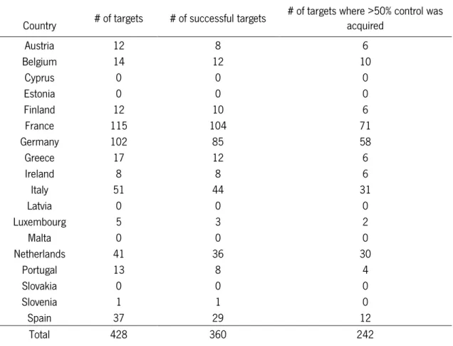
In total, the sample counts 428 targets, of which 13 are hostile targets. These targets do not have any restrictions regarding the shares that the acquirer obtains and have a deal value of at least 1 million. From the 428 targets, 360 were successful takeovers and 242 were successful and the acquirer got more than 50% control of the target firm. For the hostile targets, there are 10 successful takeovers and 5 targets, which were successful and the acquirer got more than 50%
control of the target firm. Table 1 shows the distribution of the targets by country. It can be clearly seen that France and Germany are the countries with a higher number of targets.
TABLE 1–DESCRIPTION OF THE TARGETS BY COUNTRY
Table 1 reports the total number of targets, the number of successful targets and the number of targets where the acquirer got more than 50% control, all by country. The targets were extracted from SDC Platinum and includes the 18 Euro Zone countries. The sample period is from 2000 until 2015. I exclude the financial sector and utilities which have the Standard Industry Classification (SIC) codes between 4900-4949 and 6000-6999 from the sample.
Country # of targets # of successful targets # of targets where >50% control was acquired
Austria 12 8 6 Belgium 14 12 10 Cyprus 0 0 0 Estonia 0 0 0 Finland 12 10 6 France 115 104 71 Germany 102 85 58 Greece 17 12 6 Ireland 8 8 6 Italy 51 44 31 Latvia 0 0 0 Luxembourg 5 3 2 Malta 0 0 0 Netherlands 41 36 30 Portugal 13 8 4 Slovakia 0 0 0 Slovenia 1 1 0 Spain 37 29 12 Total 428 360 242
Moreover, I use a control sample with all the public firms listed on the local exchange of each country from 2000 to 2015. These are firms which were not targets of a takeover attempt.
Table 2 shows the summary statistics of all the targets and the control sample using cash and control variables.
Table 2 shows the summary statistics of the cash and control variables from the targets and the control sample. The CashAssets is defined as Cash Short Term Invest divided by the Total Assets. The ExcessCash 1, 2 and 3 are the residual from the regression (1) predicting cash to assets. I separate the residuals of each Excess Cash by sign, so positive Excess Cash equals excess cash when the residual is positive and zero otherwise. The same for the negative Excess Cash. The CashFlowAssets is the CashFlow divided by the Total Assets. The NWCAssets is the NWC divided by the Total Assets. The control variable RealSize is the natural logarithm of the Total Assets where Total Assets are deflated into 2015 prices using the CPI. The BooktoMarket are the Total Assets divided by the Total Assets excluding the Common Equity and including the Market Value. The ROE is the Net Income divided by the Common Equity. The SalesGrowth is a ratio measured on a year-to-year basis using the Net Sales from year t minus the Net Sales from the previous year (t-1), divided by the Net Sales from the previous year (t-1). The PriorStockReturns are measured monthly using the compounded raw returns from the previous 12 months. The TotalLeverage is the Long Term Debt and the Short Term Debt divided by the Common Equity. The targets were extracted from SDC Platinum and the control sample includes all firms which were listed in the respective exchange-list. The sample period is from 2000 until 2015. The differences of means are tested using a t-test while the differences in medians are tested with a Wilcoxon rank-sum.
all Targets ControlSample Differences in Means
Differences in Medians
Variable N Mean Median Std. Dev. N Mean Median Dev. Std.
Cash Variables CashAssets 5522 0.1125 0.0794 0.1126 17457 0.1333 0.0905 0.1206 0.0208* 0.0111 ExcessCash3 5522 0.0291 0.1321 1.1109 17457 -0.0092 0.1429 1.1857 -0.0383** 0.0108 ExcessCash2 4628 0.0469 0.1746 0.9913 12926 -0.0168 0.1392 1.0568 -0.0637*** -0.0354*** ExcessCash1 4483 0.0484 0.1812 0.9847 12635 -0.0172 0.1329 1.0516 -0.0656*** -0.0483*** CashFlowAssets 5249 0.0476 0.0556 0.0806 16791 0.0559 0.05973 0.0646 0.0083*** 0.00413 NWCAssets 5357 -0.0148 -0.0166 0.1772 17078 0.0101 0.0058 0.1651 0.0249*** 0.0224*** Control Variables RealSize 5531 13.5966 13.3088 1.6156 17462 14.9572 14.2787 1.8366 1.3606** 0.9699 BooktoMarket 4996 1.8303 1.5082 1.0791 13695 1.9219 1.6052 1.0988 0.0916*** 0.0970*** ROE 5537 0.0318 0.0801 0.4028 17478 0.0651 0.0946 0.3556 0.0333*** 0.0145*** SalesGrowth 5269 0.1221 0.0486 0.6272 16900 0.0951 0.0314 0.5611 -0.0270*** -0.0172*** PriorStockReturns 10796 0.0005 0.01 0.1175 37798 0.2839 0,0000 1.8862 0.2834*** -0.0100*** TotalLeverage 5441 1.2483 0.7561 2.0322 17291 1.1297 0.6577 1.8689 -0.1186*** -0.0984***
Robust z-statistics in parentheses *** p<0.01, ** p<0.05, * p<0.1
I use the t-test for the difference of means between the two groups, and the t-Wilcoxon test for the difference of medians. The Cash variable is not the same in the two groups, the control sample seems to hold more cash than the targets. In contrast, there are some significant differences for the Excess Cash. Excess Cash 3, which includes just the Size and Industry Sigma, is higher in the median for the control sample than for the other targets. This difference is just significant at the mean. For the Excess Cash 2, which excludes just the Cash Flow, and the Excess Cash 1, which includes all the variables of the Excess Cash regression, it is the other way around. The targets seem to hold more cash than the non-targets with significant difference at mean and median. On the other hand, the Cash Flow and NWC are higher for the control sample than for the targets, with significant difference at the mean on the Cash Flow and significant difference at the mean and median on the NWC. The cash variables lead us to different conclusions. The Cash seems to contradict the conventional wisdom whereas the various Excess Cash seem to support it. However, this analysis is only univariate and has to be complemented with the multivariate analysis, in which I use different variables of the same regression in order to test whether the different cash variables have any different impact on the results.
Regarding the control variables, the Size is lower for the targets than for the control sample and their difference is significant just on the mean. The Book-to-Market is for all targets smaller than for the control sample, whose difference is significant at the mean and median. The same is noticeable for the ROE regarding the significant mean and median. For the Sales Growth, exactly the opposite is observable. For the targets, the Sales Growth is higher than the one of the control sample with significant difference in the mean and median. The Prior Stock Returns do not show a noticeable difference between the two groups in contrast to the Total Leverage. The control variable Total Leverage has a significant difference, both in the mean and median, by showing higher values for the targets than for the non-targets. The control variables Book-to-Market, ROE, Sales Growth and Total Leverage are different for targets and non-targets. Also, this conclusion is just based on a univariate analysis and has to be tested through the regressions, in order to conclude consistency or not with the literature. In addition, I check if the variables are correlated with each other. Table 3 presents the correlation between all the control and cash variables of the regressions. Based on the results of this table, there should not be any problem using the variables simultaneously in the regressions, because the correlation is not very high.
Table 3 presents the correlations among the cash and control variables. The ROE is the Net Income divided by the Common Equity. The SalesGrowth is a ratio measured on a year-to-year basis using the Net Sales from year t minus the Net Sales from the previous year (t-1), divided by the Net Sales from the previous year (t-1). The NWCAssets is the NWC divided by the Total Assets. The TotalLeverage is the Long Term Debt and the Short Term Debt divided by the Common Equity. The BooktoMarket are the Total Assets divided by the Total Assets excluding the Common Equity and including the Market Value. The control variable RealSize is the natural logarithm of the Total Assets where Total Assets are deflated into 2015 prices using the CPI. The CashFlowAssets is the CashFlow divided by the Total Assets. The PriorStockReturns are measured monthly using the compounded raw returns from the previous 12 months. The CashAssets is defined as Cash Short Term Invest divided by Total Assets. The ExcessCash 1, 2 and 3 are the residual from the regression (1) predicting cash to assets. I separate the residuals of each Excess Cash by sign, so positive Excess Cash equals excess cash when the residual is positive and zero otherwise. The same for the negative Excess Cash. The numbers which are presented in parentheses are the p-values, testing that the correlation equals 0.
ROE Growth Sales Assets NWC Leverage Total Bookto Market Real Size CashFlow Assets PriorStock Returns Assets Cash Excess Cash3 Excess Cash2 ROE Sales Growth 0.0285 (0.0000) NWC Assets 0.0654 (0.0000) 0.0152 (0.0000) Total Leverage (0.0000) -0.3773 (0.0000) 0.0229 (0.0000) -0.2108 Bookto Market 0.0521 (0.0000) 0.0310 (0.0000) 0.2827 (0.0000) -0.2883 (0.0000) Real Size (0.0000) 0.0820 (0.0000) 0.0217 (0.0000) -0.1886 (0.0000) 0.1705 (0.0000) -0.1880 CashFlow Assets (0.0000) 0.4261 (0.0000) 0.0373 (0.0000) 0.1676 (0.0000) -0.1163 (0.0000) 0.0798 (0.0000) 0.0747 PriorStock Returns 0.0922 (0.0000) 0.0039 (0.0000) 0.0761 (0.0000) -0.0740 (0.0000) 0.0631 (0.0000) 0.0446 (0.0000) 0.1280 (0.0000) Cash Assets 0.0613 (0.0000) 0.0308 (0.0000) -0.0814 (0.0000) -0.1471 (0.0000) 0.3452 (0.0000) -0.0773 (0.0000) 0.0235 (0.0005) 0.0701 (0.0000) Excess Cash3 0.0583 (0.0000) 0.0180 (0.0074) -0.0703 (0.0000) -0.0998 (0.0000) 0.1493 (0.0000) 0.0000 (0.0000) 0.0347 (0.0000) 0.0297 (0.0000) 0.7627 (0.0000) Excess Cash2 (0.0000) 0.0433 (0.0000) 0.0493 (0.0000) 0.0007 (0.0000) 0.0002 (0.0006) 0.0258 (0.0000) 0.0000 (0.0000) 0.0316 (0.0000) 0.0397 (0.0000) 0.6634 (0.0000) 0.9412 Excess Cash1 (0.0000) 0.0311 (0.0000) 0.0509 (0.0000) 0.0005 (0.0000) 0.0010 (0.0001) 0.0294 (0.0000) 0.0004 (0.0000) 0.0002 (0.0000) 0.0386 (0.0000) 0.6661 (0.0000) 0.9412 (0.0000) 0.9992
5. Results
5.1. Probability of an acquisition
In this section, I test whether firms with higher levels of cash holdings are less likely to be acquired in a takeover bid. Nevertheless, as I mention in the previous section, I test every regression with different combinations of variables in order to examine whether there is any difference. In addition, to get more precise results, I include in every single regression the fixed effect of industry (using the 2-digit SIC code), target nation and year. The probit regression that I use to determine the probability of acquisition, which corresponds to my hypothesis H1A, is equation (2). In this regression, the dependent variable equals 1 if the target was successfully acquired and 0 otherwise. It is defined as successful when a firm was acquired by any bidder.
The results are presented in Table 4 using 360 targets and where columns (1) to (4) exclude the control variables Cash Flow and NWC and each column includes one different cash variable. From column (5) to (8) all control variables are included and once again each column tests one different cash variable. It is observable that in the interest variables, there is no significant value for Cash. However, the positive Excess Cash 3 is negative and significant by including the Cash Flow and NWC. Negative Excess Cash 1, 2 and 3 are positive and significant, which means that firms with too little cash are less likely to be acquired. This is not consistent with the positive Excess Cash 3, which is negative and significant, and shows that firms with excess cash are less likely to be acquired. Regarding the control variables, it is observable that the Sales Growth has a positive relationship with the probability of being acquired. In other words, the higher the Sales Growth, the higher the probability of a firm being acquired. Having a positive sales growth is a sign of a good management and seems to attract acquirers. The same positive relationship I find with the Size of the firm. The larger the firm, the higher the probability of it being acquired.
TABLE 4–PROBIT REGRESSION FOR THE LIKELIHOOD OF BEING ACQUIRED
Table 4 exhibits the results of the probit regression (2) with the dependent variable being equal to 1 if an announced target is a successful takeover and 0 otherwise. A takeover is defined as successful when the target firm was acquired by any bidder. The sample includes all successful takeover targets from 2000 until 2015, reported by SDC Platinum. The control sample includes all exchange listed firms, in the respective countries, from 2000 to 2015. The ROE is the Net Income divided by the Common Equity. The SalesGrowth is a ratio measured on a year-to-year basis using the Net Sales from year t minus the Net Sales from the previous year 1), divided by the Net Sales from the previous year (t-1). The TotalLeverage is the Long Term Debt and the Short Term Debt divided by the Common Equity. The BooktoMarket are the Total Assets divided by the Total Assets excluding the Common Equity and including the Market Value. The control variable RealSize is the natural logarithm of the Total Assets where Total Assets are deflated into 2015 prices using the CPI. The PriorStockReturns are measured monthly using the compounded raw returns from the previous 12 months. The CashFlowAssets is the CashFlow divided by the Total Assets. The NWCAssets is the NWC divided by the Total Assets. The CashAssets is defined as Cash Short Term Invest divided by the Total Assets. The positive and negative ExcessCash 1, 2 and 3 are the residual from the regression (1) predicting cash to assets, I separate the residuals of each Excess Cash by sign, so positive Excess Cash equals excess cash when the residual is positive and zero otherwise. The same for the negative Excess Cash. The numbers which are presented in parentheses are z-statistics with standard errors. The regression includes the fixed effects industry, country and year.
VARIABLES (1) (2) (3) (4) (5) (6) (7) (8) ROE 0.0081 0.0085 -0.0005 -0.0001 -0.0026 -0.0019 -0.0059 -0.0059 (0.46) (0.92) (-0.05) (-0.01) (-0.18) (-0.19) (-0.58) (-0.58) SalesGrowth 0.0177*** 0.0177*** 0.0199*** 0.0229*** 0.0200*** 0.0197*** 0.0228*** 0.0228*** (3.61) (3.44) (3.34) (3.68) (3.75) (3.43) (3.70) (3.69) TotalLeverage 0.0022 0.0025 -0.0006 -0.0000 -0.0010 -0.0008 -0.0013 -0.0013 (0.52) (1.32) (-0.30) (-0.02) (-0.25) (-0.40) (-0.69) (-0.68) BooktoMarket -0.0039 -0.0021 -0.0062* -0.0052 -0.0007 0.0008 -0.0008 -0.0009 (-0.65) (-0.63) (-1.82) (-1.52) (-0.09) (0.23) (-0.23) (-0.26) RealSize 0.0089 0.0081*** 0.0088*** 0.0089*** 0.0072 0.0060*** 0.0070*** 0.0070*** (1.52) (4.34) (4.67) (4.70) (1.27) (3.11) (3.69) (3.68) PriorStockReturns -0.0833*** -0.0833*** -0.0843*** -0.0839*** -0.0804*** -0.0802*** -0.0825*** -0.0826*** (-8.63) (-40.03) (-39.82) (-39.39) (-7.89) (-37.77) (-38.16) (-38.16) ExCash3Positive -0.0008 -0.0108* (-0.12) (-1.65) ExCash3Negative 0.0138*** 0.0206*** (3.24) (4.43) CashAssets 0.0571 0.0168 (0.75) (0.21) ExCash2Positive 0.0110 0.0075 (1.61) (1.08) ExCash2Negative 0.0116** 0.0138*** (2.52) (2.93) ExCash1Positive 0.0103 0.0080 (1.49) (1.16) ExCash1Negative 0.0121*** 0.0135*** (2.58) (2.87) CashFlowAssets 0.0761 0.0714 0.0799* 0.0847* (0.87) (1.56) (1.73) (1.83) NWCAssets -0.1239** -0.1290*** -0.1186*** -0.1186*** (-2.39) (-6.46) (-5.99) (-5.99) Observations 17,087 17,087 16,333 15,955 16,244 16,244 15,955 15,955 Pseudo R-squared 0.0773 0.0778 0.0826 0.0831 0.0823 0.0834 0.0853 0.0853 Actual Prob. 0.230 0.230 0.228 0.227 0.226 0.226 0.227 0.227
Robust z-statistics in parentheses *** p<0.01, ** p<0.05, * p<0.1
This conclusion contradicts the argument of Ambrose & Megginson (1992), whereas Couderc (2005) finds that the Size influences positively the cash holdings. However, the control variable Prior Stock Returns shows exactly the opposite. There is a negative relationship between the variable and the probability of being acquired. This might be because of bad management and, consequently, the shareholders are dissatisfied. Moreover, the results of Table 4 also show a negative relationship with the NWC. This means that the NWC reduces the probability of a firm being acquired.
In addition, to test my hypothesis H1B, I include an interaction variable which consists of the multiplication of a dummy variable, called BM, and the Excess Cash, both the positive and the negative one. To calculate this variable, I sort the firms by year and Book-to-Market and create the dummy BM which equals 1 if a firm is in the highest quartile of the Book-to-Market for that year and 0 otherwise. The variables of the probit regression and the dependent variable remain unchanged. The aim is to verify whether cash rich firms with poor investments opportunities are more likely to be acquired.
TABLE 5–PROBIT REGRESSION IN DETERMINING THE LIKELIHOOD OF BEING ACQUIRED FOR FIRMS WITH POOR INVESTMENT OPPORTUNITIES
Table 5 presents the results of the probit regression (2) with the dependent variable being equal to 1 if an announced target is a successful takeover and 0 otherwise. A takeover is defined as successful when the target firm was acquired by any bidder. The sample includes all successful takeover targets from 2000 until 2015 with poor investment opportunities, reported by SDC Platinum. The control sample includes all exchange listed firms, in the respective countries, from 2000 to 2015. The ROE is the Net Income divided by the Common Equity. The SalesGrowth is a ratio measured on a year-to-year basis using the Net Sales from year t minus the Net Sales from the previous year (t-1), divided by the Net Sales from the previous year (t-1). The TotalLeverage is the Long Term Debt and the Short Term Debt divided by the Common Equity. The BooktoMarket are the Total Assets divided by the Total Assets excluding the Common Equity and including the Market Value. The control variable RealSize is the natural logarithm of the Total Assets where Total Assets are deflated into 2015 prices using the CPI. The PriorStockReturns are measured monthly using the compounded raw returns from the previous 12 months. The CashFlowAssets is the CashFlow divided by the Total Assets. The NWCAssets is the NWC divided by the Total Assets. The CashAssets is defined as Cash Short Term Invest divided by the Total Assets. The positive and negative ExcessCash 1, 2 and 3 are the residual from the regression (1) predicting cash to assets, I separate the residuals of each Excess Cash by sign, so positive Excess Cash equals excess cash when the residual is positive and zero otherwise. The same for the negative Excess Cash. The interaction variable is the multiplication of the dummy BM and the (positive and negative) Excess Cash. BM is a dummy which equals 1 if the firm is in the highest year of Book to Market of all firms for that year and 0 otherwise. The numbers which are presented in parentheses are z-statistics with standard errors. The regression includes the fixed effects industry, country and year. The variables ROE, TotalLeverage and the positive and negative Excess Cash variables are not illustrated on the table, because they are not relevant for the conclusions of this specific table.
VARIABLES (1) (2) (3) (4) (5) (6) (7) (8) … … … … SalesGrowth 0.0187*** 0.0186*** 0.0210*** 0.0242*** 0.0226*** 0.0222*** 0.0241*** 0.0241*** (3.61) (3.30) (3.21) (3.53) (3.92) (3.53) (3.55) (3.54) … … … … …. … … … … BooktoMarket -0.0016 -0.0012 -0.0079** -0.0067* 0.0008 0.0003 -0.0028 -0.0028 (-0.22) (-0.33) (-2.11) (-1.79) (0.10) (0.08) (-0.75) (-0.75) RealSize 0.0033 0.0031 0.0043** 0.0040** 0.0019 0.0008 0.0021 0.0020 (0.48) (1.55) (2.12) (1.99) (0.28) (0.39) (1.00) (1.00) PriorStockReturns -0.0917*** -0.0918*** -0.0929*** -0.0925*** -0.0887*** -0.0887*** -0.0911*** -0.0912*** (-8.34) (-41.26) (-40.80) (-40.40) (-7.87) (-39.08) (-39.33) (-39.34) … … … BM*ExCash3Positive -0.0449*** -0.0328** (-3.51) (-2.50) … … … BM*ExCash3Negative 0.0080 -0.0073 (0.99) (-0.82) … … … BM*CashAssets -0.2812* -0.2350 (-1.80) (-1.52) … … … BM*ExCash2Positive -0.0315*** -0.0287** (-2.65) (-2.35) … … … BM*ExCash2Negative -0.0006 -0.0084 (-0.07) (-0.85) … … … BM*ExCash1Positive -0.0325*** -0.0289** (-2.70) (-2.37) … … … BM*ExCash1Negative 0.0004 -0.0078 (0.04) (-0.79) CashFlowAssets 0.0761 0.0570 0.0737 0.0795 (0.84) (1.18) (1.51) (1.62) NWCAssets -0.1240** -0.1367*** -0.1265*** -0.1265*** (-2.36) (-6.46) (-6.03) (-6.03) Observations 17,954 17,954 17,137 16,737 17,051 17,051 16,737 16,737 Pseudo R-squared 0.0761 0.0760 0.0821 0.0825 0.0813 0.0820 0.0845 0.0845 Actual Prob. 0.265 0.265 0.262 0.261 0.260 0.260 0.261 0.261
Table 5 presents the results of the probability of acquisitions for firms with poor investments opportunities. In this table, the three positive interaction variables (BM*ExCash1Positive, BM*ExCash2Positive and BM*ExCash3Positive) are negative and significant and leave no room for doubt, as in the previous table, that firms with higher cash holdings are less likely to be acquired. In contrast to the previous table, the variable Cash is negative and significant, but just when excluding the variables Cash Flow and NWC. This shows evidence that the market for corporate control does not monitor cash holdings. The other interest variables on the table do not change sign or its significance level is barely changed by including or excluding Cash Flow and NWC. Regarding the control variables, when the probability of being acquired equals one, the increase in the likelihood is on average of 2.19 percentage points, ceteris paribus, when the variable Sales Growth goes up by one unit. Moreover, there is a negative relationship with Prior Stock Returns and NWC in relation to the probability of being acquired. To examine whether the market of corporate control monitors the firms’ cash holdings even when the targets lose their independence, I rerun the probabilistic regression using the successful acquisitions and where the bidder gained more than 50% control of the target firm. More specifically, there are 242 targets with these criteria and those results are shown in Table 6.
TABLE 6–PROBIT REGRESSION DETERMINING THE LIKELIHOOD OF BEING ACQUIRED AND GAINING CONTROL
Table 6 exhibits the results of the probit regression (2) with the dependent variable being equal to 1 if an announced target is a successful takeover and the acquirer got control and 0 otherwise. A takeover is defined as successful when the target firm was acquired by any bidder. The sample includes all successful takeover targets and where the bidder got more than 50% of control over the target, from 2000 until 2015, reported by SDC Platinum. The control sample includes all exchange listed firms, in the respective countries, from 2000 to 2015. The ROE is the Net Income divided by the Common Equity. The SalesGrowth is a ratio measured on a year-to-year basis using the Net Sales from year t minus the Net Sales from the previous year (t-1), divided by the Net Sales from the previous year (t-1). The TotalLeverage is the Long Term Debt and the Short Term Debt divided by the Common Equity. The BooktoMarket are the Total Assets divided by the Total Assets excluding the Common Equity and including the Market Value. The control variable RealSize is the natural logarithm of the Total Assets where Total Assets are deflated into 2015 prices using the CPI. The PriorStockReturns are measured monthly using the compounded raw returns from the previous 12 months. The CashFlowAssets is the CashFlow divided by the Total Assets. The NWCAssets is the NWC divided by the Total Assets. The CashAssets is defined as Cash Short Term Invest divided by the Total Assets. The positive and negative ExcessCash 1, 2 and 3 are the residual from the regression (1) predicting cash to assets. I separate the residuals of each Excess Cash by sign, so positive Excess Cash equals excess cash when the residual is positive and zero otherwise. The same for the negative Excess Cash. The numbers which are presented in parentheses are z-statistics with standard errors. The regression includes the fixed effects industry, country and year.
VARIABLES (1) (2) (3) (4) (5) (6) (7) (8) ROE 0.0245* 0.0253*** 0.0181** 0.0177** 0.0133 0.0146* 0.0129 0.0129 (1.95) (3.29) (2.36) (2.31) (1.39) (1.77) (1.56) (1.56) SalesGrowth 0.0070* 0.0070* 0.0098** 0.0115** 0.0089** 0.0087* 0.0113** 0.0113** (1.85) (1.72) (2.20) (2.48) (2.51) (1.95) (2.44) (2.44) TotalLeverage 0.0049* 0.0052*** 0.0026* 0.0031** 0.0023 0.0026* 0.0022 0.0022 (1.66) (3.45) (1.68) (2.03) (0.89) (1.68) (1.44) (1.44) BooktoMarket 0.0022 0.0035 -0.0022 -0.0013 0.0023 0.0037 0.0011 0.0011 (0.39) (1.29) (-0.82) (-0.47) (0.30) (1.27) (0.40) (0.40) RealSize -0.0076* -0.0083*** -0.0087*** -0.0083*** -0.0093** -0.0104*** -0.0095*** -0.0095*** (-1.66) (-5.31) (-5.61) (-5.40) (-2.06) (-6.60) (-6.01) (-6.03) PriorStockReturns -0.0502*** -0.0500*** -0.0492*** -0.0485*** -0.0467*** -0.0463*** -0.0476*** -0.0476*** (-7.78) (-33.01) (-32.80) (-32.37) (-6.84) (-30.44) (-30.92) (-30.93) ExCash3Positive -0.0111** -0.0173*** (-2.12) (-3.24) ExCash3Negative 0.0119*** 0.0211*** (3.40) (5.38) CashAssets -0.0079 -0.0156 (-0.13) (-0.26) ExCash2Positive -0.0010 -0.0032 (-0.18) (-0.57) ExCash2Negative 0.0124*** 0.0137*** (3.28) (3.55) ExCash1Positive -0.0020 -0.0034 (-0.35) (-0.60) ExCash1Negative 0.0131*** 0.0139*** (3.40) (3.58) CashFlowAssets 0.0639 0.0603 0.0595 0.0610 (0.92) (1.62) (1.60) (1.64) NWCAssets -0.0794* -0.0837*** -0.0727*** -0.0727*** (-1.86) (-5.17) (-4.54) (-4.54) Observations 15,263 15,263 14,580 14,236 14,504 14,504 14,236 14,236 Pseudo R-squared 0.0707 0.0716 0.0749 0.0745 0.0734 0.0761 0.0765 0.0765 Actual Prob. 0.143 0.143 0.140 0.138 0.137 0.137 0.138 0.138
Robust z-statistics in parentheses *** p<0.01, ** p<0.05, * p<0.1
The positive Excess Cash 3 is negative and significant, showing that excess cash defends firms from being acquired, whereas the three negative Excess Cash are positive and statistically significant at the level of 1%, indicating that firms with higher cash deficits are also less likely to be acquired. In addition, consistent with the previous tables, there is a negative relationship with Size of the firm, the Prior Stock Returns and the NWC. On the other hand, there is a positive relationship with the ROE and the Total Leverage in columns (1) to (4) and with the Sales Growth, but in columns (1) to (8).
To sum up, I conclude from Table 4, 5 and 6 that firms with more extreme cash deficits are less likely to be acquired. However, firms with poor growth opportunities are less likely to be acquired when they hold more positive excess cash. This means that I accept my hypothesis H1B, but I do not accept my hypothesis H1A.
5.2. Probability of being targeted
Apart from testing the probability of being acquired, I test the probability of a firm being targeted. The previous analyses test the probability of a firm being acquired successfully. But do excess cash holdings prevent firms from being targeted? In Table 7 I re-examine the results using the same regression as in the previous tables, but considering all targets, that is, the successful and unsuccessful ones.
TABLE 7–PROBIT REGRESSION DETERMINING THE LIKELIHOOD OF BEING TARGETED
Table 7 shows the results of the probit regression (2) with the dependent variable being equal to 1 if a firm is an announced target and 0 otherwise. The sample includes all targets, from 2000 until 2015, reported by SDC Platinum. The control sample includes all exchange listed firms, in the respective countries, from 2000 to 2015. The ROE is the Net Income divided by the Common Equity. The SalesGrowth is a ratio measured on a year-to-year basis using the Net Sales from year t minus the Net Sales from the previous year 1), divided by the Net Sales from the previous year (t-1). The TotalLeverage is the Long Term Debt and the Short Term Debt divided by the Common Equity. The BooktoMarket are the Total Assets divided by the Total Assets excluding the Common Equity and including the Market Value. The control variable RealSize is the natural logarithm of the Total Assets where Total Assets are deflated into 2015 prices using the CPI. The PriorStockReturns are measured monthly using the compounded raw returns from the previous 12 months. The CashFlowAssets is the CashFlow divided by the Total Assets. The NWCAssets is the NWC divided by the Total Assets. The CashAssets is defined as Cash Short Term Invest divided by the Total Assets. The positive and negative ExcessCash 1, 2 and 3 are the residual from the regression (1) predicting cash to assets. I separate the residuals of each Excess Cash by sign, so positive Excess Cash equals excess cash when the residual is positive and zero otherwise. The same for the negative Excess Cash. The numbers which are presented in parentheses are z-statistics with standard errors. The regression includes the fixed effects industry, country and year.
VARIABLES (1) (2) (3) (4) (5) (6) (7) (8) ROE 0.0086 0.0090 -0.0005 0.0005 0.0008 0.0015 -0.0039 -0.0039 (0.50) (0.94) (-0.05) (0.05) (0.05) (0.14) (-0.37) (-0.36) SalesGrowth 0.0189*** 0.0188*** 0.0212*** 0.0245*** 0.0229*** 0.0225*** 0.0244*** 0.0244*** (3.62) (3.35) (3.24) (3.59) (3.96) (3.60) (3.60) (3.60) TotalLeverage 0.0040 0.0042** 0.0005 0.0012 0.0005 0.0007 -0.0002 -0.0001 (0.88) (2.15) (0.22) (0.59) (0.12) (0.35) (-0.08) (-0.07) BooktoMarket -0.0065 -0.0050 -0.0099*** -0.0090** -0.0031 -0.0018 -0.0042 -0.0043 (-0.99) (-1.43) (-2.74) (-2.44) (-0.37) (-0.46) (-1.12) (-1.14) RealSize 0.0043 0.0036* 0.0047** 0.0044** 0.0026 0.0013 0.0026 0.0025 (0.63) (1.81) (2.34) (2.21) (0.38) (0.62) (1.25) (1.24) PriorStockReturns -0.0922*** -0.0921*** -0.0933*** -0.0929*** -0.0889*** -0.0886*** -0.0913*** -0.0913*** (-8.39) (-41.36) (-40.96) (-40.57) (-7.84) (-39.09) (-39.40) (-39.40) ExCash3Positive -0.0046 -0.0156** (-0.69) (-2.26) ExCash3Negative 0.0124*** 0.0221*** (2.79) (4.54) CashAssets 0.0302 -0.0058 (0.34) (-0.06) ExCash2Positive 0.0110 0.0072 (1.53) (0.99) ExCash2Negative 0.0127*** 0.0150*** (2.63) (3.03) ExCash1Positive 0.0100 0.0076 (1.37) (1.04) ExCash1Negative 0.0131*** 0.0148*** (2.67) (2.98) CashFlowAssets 0.0550 0.0502 0.0621 0.0670 (0.62) (1.05) (1.29) (1.39) NWCAssets -0.1339** -0.1384*** -0.1267*** -0.1267*** (-2.57) (-6.62) (-6.10) (-6.11) Observations 17,954 17,954 17,137 16,737 17,051 17,051 16,737 16,737 Pseudo R-squared 0.0750 0.0754 0.0817 0.0821 0.0806 0.0817 0.0841 0.0841 Actual Prob. 0.265 0.265 0.262 0.261 0.260 0.260 0.261 0.261
Robust z-statistics in parentheses *** p<0.01, ** p<0.05, * p<0.1
The negative and significant value for the positive Excess Cash 3 (including Cash Flow and NWC) proves a declining probability of being targeted holding excess cash. Furthermore, the positive and significant value at 1% for the three negative Excess Cash variables indicates that firms with more extreme cash defits are also less likely to be targeted in a takeover attempt. The positive relationship with the control variable Sales Growth and the negative relationship with the Prior Stock Returns and NWC remains.
Additionally, I test the probability of being targeted for firms with poor investment opportunities using again the interaction term. The results are in Table 8 and do not differ from the results obtained until now for this group of companies. The positive interaction variables are negative and significant at 1% and 5%, and show that cash rich firms with poor investment opportunities do not have an increased probability of being targeted. Persistently, the negative and significant BM*CashAssets variable in the first column points out that there is no monitoring of the market of corporate control.
TABLE 8–PROBIT REGRESSION DETERMINING THE LIKELIHOOD OF BEING TARGETED FOR FIRMS WITH POOR INVESTMENT OPPORTUNITIES
Table 8 presents the results of the probit regression (2) with the dependent variable being equal to 1 if a firm is an announced target and 0 otherwise. The sample includes all targets with poor investment opportunities, from 2000 until 2015, reported by SDC Platinum. The control sample includes all exchange listed firms, in the respective countries, from 2000 to 2015. The ROE is the Net Income divided by the Common Equity. The SalesGrowth is a ratio measured on a year-to-year basis using the Net Sales from year t minus the Net Sales from the previous year (t-1), divided by the Net Sales from the previous year (t-1). The TotalLeverage is the Long Term Debt and the Short Term Debt divided by the Common Equity. The BooktoMarket are the Total Assets divided by the Total Assets excluding the Common Equity and including the Market Value. The control variable RealSize is the natural logarithm of the Total Assets where Total Assets are deflated into 2015 prices using the CPI. The PriorStockReturns are measured monthly using the compounded raw returns from the previous 12 months. The CashFlowAssets is the CashFlow divided by the Total Assets. The NWCAssets is the NWC divided by the Total Assets. The CashAssets is defined as Cash Short Term Invest divided by the Total Assets. The positive and negative ExcessCash 1, 2 and 3 are the residual from the regression (1) predicting cash to assets. I separate the residuals of each Excess Cash by sign, so positive Excess Cash equals excess cash when the residual is positive and zero otherwise. The same for the negative Excess Cash. The interaction variable is the multiplication of the dummy BM and the (positive and negative) Excess Cash. BM is a dummy which equals 1 if the firm is in the highest year of Book to Market of all firms for that year and 0 otherwise. The numbers which are presented in parentheses are z-statistics with standard errors. The regression includes the fixed effects industry, country and year. The variables ROE, TotalLeverage and the positive and negative Excess Cash variables are not illustrated on the table, because they are not relevant for the conclusions of this specific table.
VARIABLES (1) (2) (3) (4) (5) (6) (7) (8) … … … … SalesGrowth 0.0187*** 0.0186*** 0.0210*** 0.0242*** 0.0226*** 0.0222*** 0.0241*** 0.0241*** (3.61) (3.30) (3.21) (3.53) (3.92) (3.53) (3.55) (3.54) … … … … BooktoMarket -0.0016 -0.0012 -0.0079** -0.0067* 0.0008 0.0003 -0.0028 -0.0028 (-0.22) (-0.33) (-2.11) (-1.79) (0.10) (0.08) (-0.75) (-0.75) RealSize 0.0033 0.0031 0.0043** 0.0040** 0.0019 0.0008 0.0021 0.0020 (0.48) (1.55) (2.12) (1.99) (0.28) (0.39) (1.00) (1.00) PriorStockReturns -0.0917*** -0.0918*** -0.0929*** -0.0925*** -0.0887*** -0.0887*** -0.0911*** -0.0912*** (-8.34) (-41.26) (-40.80) (-40.40) (-7.87) (-39.08) (-39.33) (-39.34) … … … BM*ExCash3Positive -0.0449*** -0.0328** (-3.51) (-2.50) … … … BM*ExCash3Negative 0.0080 -0.0073 (0.99) (-0.82) … … … BM*CashAssets -0.2812* -0.2350 (-1.80) (-1.52) … … … BM*ExCash2Positive -0.0315*** -0.0287** (-2.65) (-2.35) … … … BM*ExCash2Negative -0.0006 -0.0084 (-0.07) (-0.85) … … … BM*ExCash1Positive -0.0325*** -0.0289** (-2.70) (-2.37) … … … BM*ExCash1Negative 0.0004 -0.0078 (0.04) (-0.79) CashFlowAssets 0.0761 0.0570 0.0737 0.0795 (0.84) (1.18) (1.51) (1.62) NWCAssets -0.1240** -0.1367*** -0.1265*** -0.1265*** (-2.36) (-6.46) (-6.03) (-6.03) Observations 17,954 17,954 17,137 16,737 17,051 17,051 16,737 16,737 Pseudo R-squared 0.0761 0.0760 0.0821 0.0825 0.0813 0.0820 0.0845 0.0845 Actual Prob. 0.265 0.265 0.262 0.261 0.260 0.260 0.261 0.261