High-tech human capital: Do the richest countries invest the
most?
∗
Tiago Neves Sequeira
†Abstract
Research and Development (R&D) endogenous growth models predict and most evidence show that investment in R&D increase with economic development. We consider the type of human capital mainly used in research labs and show that the richest countries are investing proportionally less than middle income countries in engineering and technical human capital. We generalize this result, controlling for other explanatory variables, cross-time error correlations, heteroskedaticity and endogeneity bias. Thus, we establish a stylized fact (about human capital composition) that is a puzzle to economic theory: the ratio of high-tech to low-tech human capital presents an inverted U-shaped relationship with GDP per capita.
JEL Classification: O15, O33, O50.
Key-Words: human capital composition, high-tech human capital, R&D, Development.
1
Introduction
The study of the effects of human capital composition on growth and development is a recent field in the economic literature. The idea that some classes of human capital contribute more to growth than others is intuitive, mainly if we think about R&D models in the spirit of Romer (1990) or Grossman and Helpman (1991), because only some types of human capital are engaged in R&D activities. The first paper in this class was the seminal work of Murphy, Shleifer and Vishny (1991), which supports the idea that the allocation of talent is important for growth and bases the argument on the choice between being entrepreneur or rent-seeker. These authors proxied rent-seeking by the proportion of Law students in colleges and entrepreneurship by the proportion of Engineering students in colleges and show some evidence that the latter contribute to growth while the former do not. Barro (1999) used data on students’ scores on comparable international examinations on a growth regression and showed that scores on sciences and mathematics had a positive relationship with economic growth, but scores on the reading test were insignificantly related to growth. Also, Acemoglu (2001) shows microeconomic evidence on positive and negative relationships between some professions and the stream of wages1. This seems to be sufficient to conclude that the composition of human capital matters where growth is concerned.
∗I am grateful to the Funda¸c˜ao para a Ciˆencia e Tecnologia for financial support during the second year of my PhD program (PRAXIS XXI / BD / 21485 / 99). I am grateful to Ana Balc˜ao Reis and Jos´e Tavares for extensive discussion and suggestions and to John Huffstot for text revision. I also gratefully acknowledge participants at Internal Research Workshop at the Faculdade de Economia and Carlos Os´orio for discussion and many comments and suggestions. The usual disclaimer applies.
†Faculdade de Economia, Universidade Nova de Lisboa and Departamento de Gest˜ao e Economia, Universidade
da Beira Interior. Email: [email protected]; [email protected].
1Professions with a positive relationship with the stream of wages include Engineering and Computer Science.
The treatment of the relationship between human capital composition and development2 is even further from being exhausted in the economic literature in spite of the increasing attention by international organizations. A recent report of OECD (2001) recognizes migration of highly skilled workers as a means of circulating knowledge and promoting scientific and technological development. It also presents Eurostat figures which show that the share of Scientists and Engineers3 in all HRST (Human resources in science and technology4) was about 10% across OECD countries. The European Commission has also been concerned about the shortage of graduates in the scientific and natural specializations, stating that, “more than a quarter of the graduates of colleges and universities are from social sciences” (European Commission, 1999), recognizing that this is the largest undergraduate field in Europe. However, there is a strong belief that richer countries invest more in R&D activities than do poor and middle-income countries. This belief has been theorized by Funke and Strulik (2000), who explain that richer countries invest more in R&D than poorer ones. This allows for the prior that developed countries would invest more than other countries in engineering and technical skills.
We address the relationship between a measure of Human Capital composition and the level of development of a country and show that there is a stylized fact regarding this relationship. We will focus on the composition of Human Capital from tertiary education (Colleges and Universities)5.
2
On the relationship between high-low-tech human capital
ratio and development
We define high-tech human capital as the enrollment or graduates in engineering, mathematics and computer science fields (h) and low-tech human capital as the enrollment or graduates in all other fields of science (1 − h)6. We define the high-low-tech human capital ratio as h
1−h. We use data on enrollments and graduates from UNESCO database between 1970 and 1997.
We treat the high-low-tech human capital ratio as five-year period averages, as well as GDP
per capita7, which is measured in international constant prices, from Penn World Table. With this
we analyze each cross-section of five-year period or a system of six equations, which include nearly 100 countries in each five-year period and corresponds to a total number of observations of 622 for enrollments and 461 for graduates. Some of these observations seem to be outliers as present high values for the h/(1 − h) variable. We approach outliers in a very classical way8. This conclusion is supported with the use of Least Absolute Deviations (LAD) median regression, which we show for comparison.
Next Table shows additional motivation to the problem, showing linear correlations between regional dummies and our measure of high-tech human capital.
2In this paper, development is measured by GDP per capita. This is, of course, a restrictive measure, but it is
commonly used in the cited literature.
3Isco 2 and isco 3.
4Which includes isco 2, 3 and 4.
5This does not mean that human capital composition is important only at this level. Nevertheless, due to
availabil-ity of data, we test human capital composition only at this level. See Bertochi and Spaggat (1998) for some evidence on Secondary education level.
6See data description in Appendix B. In order to avoid scientific notation in tables, we have multiplied the dependent
variable by 10.000.000.
7This approach, which limits the potential for measurement error and business cycle effects, will be extended to
some other variables in this work. Others will be considered in the initial year of each period.
8We exclude observations which are greater than q
0.75+ 1.5(q0.75− q0.25), where qiis the quantile of order i. This leads to the exclusion of observations of h above 0.462 when h was measured by enrollment and above 0.49 when h was measured by graduates.
Table 1: Human Capital Composition across the world
North America -3%
West Europe 4%
East Asia/Pacific 12%
East Europe and Central Asia 39%
Latin America/Caribbean 11%
South Asia -10%
Middle East and North Africa -7%
Sub-Saharian Africa -33%
Note: figures are correlations between a regional dummy and high-low-tech ratio.
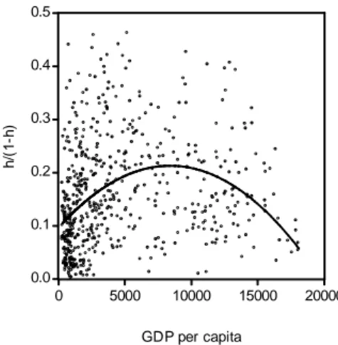
We found an inverted U-shaped relationship between h/(1 − h) and GDP per capita, which may be considered as a stylized fact because it is robust to different definitions of h/(1−h) (enrollment or graduates), different samples (total and excluding outliers) and all cross-section samples, consisting of each five-year period. This means that richer countries are investing less than middle income countries in high-tech human capital, which was not expected. We will document this relationship and test its robustness introducing controls and using instrumental variables and multiple equation methods. We will search for variables other than GDP, which may explain the high-low-tech ratio and eliminate the puzzle. Next, we show a figure with the sample excluding outliers and a polynomial adjustment. 0.0 0.1 0.2 0.3 0.4 0.5 0 5000 10000 15000 20000 GDP per capita h /( 1 -h )
Figure 1 - Polynomial Relationship
It is clear that as countries get richer the high to low tech ratio increases in developing stages and slows down or decreases in the most developed stages.
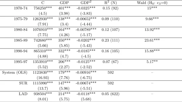
In Tables 2 and 3 we show results for OLS, LAD and SUR joint estimation of a polynomial rela-tionship between high-low-tech ratio and GDP per capita considering Enrollments and Graduates, respectively, as a measure to the cited ratio. SUR estimates allow the presence of a heteroskedastic error structure and cross-correlations of the error between equations. LAD (Least absolute devia-tions) estimates shows results’ robustness to the presence of outliers. In each regression, we present the Wald statistic and p-value for testing the null of a zero coefficient of GDP per capita squared. High-values of this statistic show that the introduction of GDP squared in the regression improves
its explanation power. We also add information about significant Wald tests on similar coefficients along time in Tables 2.1. and 3.1.
Table 2 - The Polynomial Relationship betweenh/(1 − h)and GDP (Enrollments)
C GDP GDP2 R2 (N) Wald (H0: c3=0) 1970-74 756250*** 401*** -0.0325*** 0.15 (92) 15*** (4.5) (3.98) (-3.83) 1975-79 1262930*** 138*** -0.00652*** 0.09 (110) 9.66*** (7.91) (3.4) (-4.44) 1980-84 1076910*** 164*** -0.00789*** 0.12 (107) 13.92*** (7.75) (4.26) (-5.17) 1985-89 742680*** 350*** -0.0202*** 0.23 (111) 23.61*** (5.66) (5.85) (-5.43) 1990-94 865310*** 332*** -0.0185*** 0.16 (105) 15.88*** (4.88) (4.7) (-4.5) 1995-97 1353910*** 206*** -0.0125*** 0.07 (67) 5.17** (5.52) (2.27) (-2.52) System (OLS) 1123830*** 179*** -0.00916*** 592 – (16.93) (7.76) (-6.75) SUR 1115990*** 147*** -0.00674*** 592 – (13.7) (5.96) (-5.51) LAD 938504*** 214*** -0.0118*** 0.05 (622) – (8.01) (5.75) (5.68)
Note: t-statistics based on heteroskedastic-consistent variance matrix. are presented in parentheses. Acceptable statistics (rejection of the null) are signaled with * (10%), ** (5%) and *** (1%).
Table 2.1. - Wald Tests
H0: All c1 equal 9.5* H0: c2(7074)=c2(7579)=c2(9094)=c2(9597) c2(8084)=c2(8589) 5.96 0.03 H0: c3(7074)=c3(8589)=c3(9094)=c3(9597) c3(7579)=c3(8084) 4.11 0.21
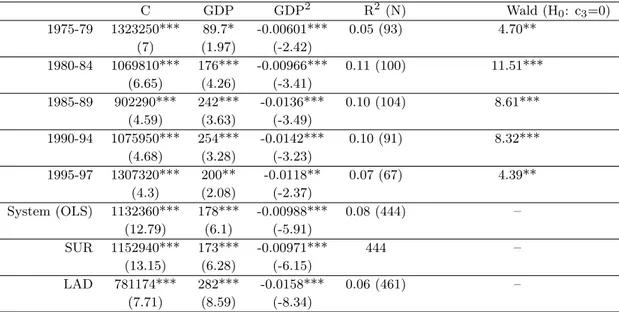
Table 3 - The Polynomial Relationship betweenh/(1 − h)and GDP (Graduates) C GDP GDP2 R2 (N) Wald (H0: c3=0) 1975-79 1323250*** 89.7* -0.00601*** 0.05 (93) 4.70** (7) (1.97) (-2.42) 1980-84 1069810*** 176*** -0.00966*** 0.11 (100) 11.51*** (6.65) (4.26) (-3.41) 1985-89 902290*** 242*** -0.0136*** 0.10 (104) 8.61*** (4.59) (3.63) (-3.49) 1990-94 1075950*** 254*** -0.0142*** 0.10 (91) 8.32*** (4.68) (3.28) (-3.23) 1995-97 1307320*** 200** -0.0118** 0.07 (67) 4.39** (4.3) (2.08) (-2.37) System (OLS) 1132360*** 178*** -0.00988*** 0.08 (444) – (12.79) (6.1) (-5.91) SUR 1152940*** 173*** -0.00971*** 444 – (13.15) (6.28) (-6.15) LAD 781174*** 282*** -0.0158*** 0.06 (461) – (7.71) (8.59) (-8.34)
Note: t-statistics based on heteroskedastic-consistent variance matrix. are presented in parentheses. Acceptable statistics (rejection of the null) are signaled with * (10%), ** (5%) and *** (1%).
Table 3.1. - Wald Tests
H0: All c1equal All c2 equal All c3 equal
2.95 4.77 3.52
The overall conclusion is that not only does this relationship seem to be qualitatively similar across time, it also presents quantitative regularities. The presence of all observations in the sample (including outliers) does not change this result, either considering enrollments or graduates as a measure of the high-low-tech ratio. In fact, even similar coefficients across time may be accepted at high statistical significance. By now, we have made our main point: there is an unexpected decrease of high-low-tech ratio in developed countries. From here on, we will test if this relationship may be considered as a puzzle in light of endogenous growth theory or, on the contrary, may be explained using the channels through which high-low-tech ratio may be affected. In testing for robustness of this relationship, we will use only enrollments, as we have more observations on this measure, and in the limit the two measures represent the same phenomenon.
3
Robustness
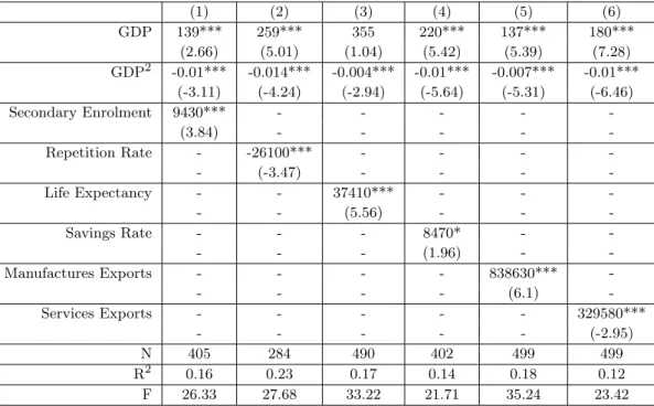
In Table 1.A (in the appendix) we perform a specification search and show the significant additional variables (other variables tested did not weaken the significance of GDP and GDP squared). We have used three types of variables other than GDP: (1) preference variables, which intend to measure high preference for the future of investors in high-tech human capital, assuming that this type of human capital has additional costs (at least opportunity costs) to be accumulated, (2) demand variables and (3) secondary education variables, measuring quantity and quality in the previous stage of education. It can be said that group (2) represents the demand side and groups (1) and (3) represent the supply side in the market for high-tech human capital. It is quite natural that some of these variables should appear in lagged periods, as variables linked to secondary schooling, which should influence the tertiary education variable in later periods.
As we want to study the relationship between h/(1 − h) ratio and GDP per capita, we will present either polynomial or linear relationships with GDP. This means that when the coefficients GDP squared are not statistically different from zero, we will present the linear relationship. In fact, in most cases, we found a clearer negative relationship between our measure of high-low-tech ratio and GDP per capita. The specification test leads to the following benchmark specification.
ht
1 − ht = β0+β1GDPt+β2GDP 2
t+β3SecEnrolt−1+β4Rpt−1+β5Elif et+β6Savt−1+
+β7M ant−1+ β8Servt−1+ε, if β26= 0
or (1)
ht
1 − ht = β0+β1GDPt+β3SecEnrolt−1+β4Rpt−1+β5Elif et+β6Savt−1+ +β7M ant−1+ β8Servt−1+ε, if β2= 0
where SecEnrol stands for enrollment in secondary schools, Rp stands for repetition rate in secondary schools, Elif e for life expectancy, Sav for savings rate, M an for the industry specialization dummy and Serv for services specialization dummy. Life expectancy is introduced in the first year of the period, GDP is introduced as an average across the period, savings rate as average across the previous period, and all the other variables were introduced as the value in the first year of the previous period9.
Following this, in Table 3, we test the robustness of the selected specification to the introduction of geographical and institutional background dummies, to possible heteroskedacity on the error dimension driven by the existence of possible outliers and also to the consideration of: (1) error-correlation between decades and (2) some possible endogeneity bias in GDP per capita.
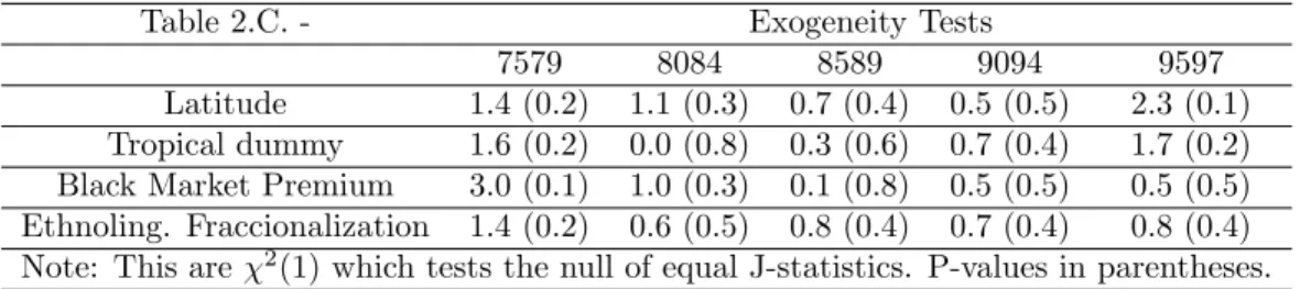
In performing instrumentation, we used a set of typically exogenously seen variables, such as geographical (longitude, latitude, dummy of tropical countries, landlocked countries), institutional (black market premium and ethnolinguistic fractionalization) and economic (exports specialization in primary fuel and non-fuel products)10. We then regress GDP per capita in those variables (as we want to instrument GDP per capita) and selected those which have statistically positive coefficients at 5% level. An overall regression of GDP per capita in these proposed instruments accounts for nearly 50% of its variation. The selected instruments were latitude, dummy of tropical countries, black market premium and etholinguistic fraccionalization. We validate this approach econometrically using a chi-squared distribution statistic which compares the J-statistic of an efficient 2SLS and a restricted J-statistic, where each of the potential endogenous instruments is omitted. According to this procedure, all the used instruments are exogenous in the presented regression at high levels of rejection of equal J-statistics11. The two instrumental estimators that we use (2SLS and 3SLS) achieve consistency through instrumentation and efficiency through appropriate weighting.
9Variables on secondary education (from Barro and Lee (2000)) are available only for some years, corresponding
to half decades (i.e. 1970 , 1975,...) until 1990. As M an and Serv are fixed, it is indifferent to introduce it in the t period or in the previous one.
10For a similar procedure, using exogenous religious and cultural variables, see Tavares and Wacziarg (2001) and
LaPorta et al. (1998).
11J-statistics are Haussman tests. See Hayashi (2000) for the proof of this test. See Tables 1.C. and 2.C in Appendix
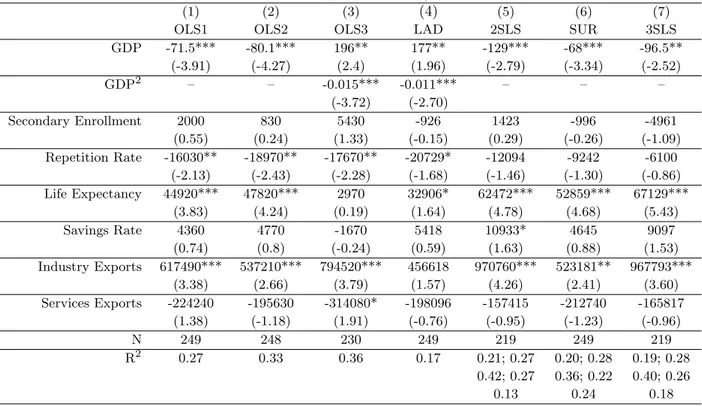
Table 4 - The possible explanation for high-low-tech ratio
(1) (2) (3) (4) (5) (6) (7)
OLS1 OLS2 OLS3 LAD 2SLS SUR 3SLS
GDP -71.5*** -80.1*** 196** 177** -129*** -68*** -96.5** (-3.91) (-4.27) (2.4) (1.96) (-2.79) (-3.34) (-2.52) GDP2 – – -0.015*** -0.011*** – – – (-3.72) (-2.70) Secondary Enrollment 2000 830 5430 -926 1423 -996 -4961 (0.55) (0.24) (1.33) (-0.15) (0.29) (-0.26) (-1.09) Repetition Rate -16030** -18970** -17670** -20729* -12094 -9242 -6100 (-2.13) (-2.43) (-2.28) (-1.68) (-1.46) (-1.30) (-0.86) Life Expectancy 44920*** 47820*** 2970 32906* 62472*** 52859*** 67129*** (3.83) (4.24) (0.19) (1.64) (4.78) (4.68) (5.43) Savings Rate 4360 4770 -1670 5418 10933* 4645 9097 (0.74) (0.8) (-0.24) (0.59) (1.63) (0.88) (1.53) Industry Exports 617490*** 537210*** 794520*** 456618 970760*** 523181** 967793*** (3.38) (2.66) (3.79) (1.57) (4.26) (2.41) (3.60) Services Exports -224240 -195630 -314080* -198096 -157415 -212740 -165817 (1.38) (-1.18) (1.91) (-0.76) (-0.95) (-1.23) (-0.96) N 249 248 230 249 219 249 219 R2 0.27 0.33 0.36 0.17 0.21; 0.27 0.20; 0.28 0.19; 0.28 0.42; 0.27 0.36; 0.22 0.40; 0.26 0.13 0.24 0.18
Notes: t-statistics are based on heteroskedastic-consistent variance matrix. Column (2) includes legal origin controls and (3) includes geografical controls. Coefficients were omitted but are available upon request. Models include an omitted constant.
In the first three columns we present OLS estimation for benchmark specification, introduction of legal origin controls (column 2) and geographical controls (column 3). In column 4, we show a median regression (Least Absolute Deviation). In column 5, we estimate 2SLS coefficients in order to account for endogeneity bias. However, there is a scope for inefficiency because this do not take into account the cross-orthogonalities between equations. Then, we estimate a SUR system which allows for cross-error correlations, in column 6. In the last column, we present 3SLS estimates which impose cross-orthogonalities and allow for endogeneity. Comparison between column (1) and (5) or between (6) and (7) gives us the benefits of accounting for endogeneity and comparison between columns (1) and (6) or between (5) and (7) gives us the efficiency gain from exploring cross-orthogonalities.
There may be some omitted variables in this regression correlated with development that could account for this strange relationship between high-low-tech ratio and GDP per capita. In spite of that, we discovered that accounting for this kind of phenomenon, the relationship between h/(1 − h) and development turns out to be negative. This means that, conditional to some variables linked with education level, education quality, intertemporal preferences and demand for high and low tech workers and eventual endogeneity, high-low-tech ratio decreases as a country develops.
We achieve some other interesting results. The high-low-tech ratio increases due to life expectancy and manufactures specialization in exports and decreases due to the level of development and possibly (with lower statistical significance) due to repetition rate at secondary school levels. As Barro and Sala-i-Martin (1995) mention “higher life expectancy may go along with better work habits and a higher level of skills” but may be also related with higher present value of future earnings12. The
manufactures dummy accounts for demand for high-tech work, which occurs mainly in industrial firms. The notion that high-tech fields are more costly to attend is captured by the negative sign of the repetition rate. Also the positive signs of life expectancy and the savings rate suggest a costly investment in high-tech human capital, which is only profitable when people have high present value of future profits or low discount rates for the future. This may be linked with a greater preference for the future in the countries that have a greater high-low-tech human capital ratio. In fact, high-tech programs are, in general, lengthier and more expensive or difficult, which means that these types of program are a higher lifetime investment than other low-tech types.
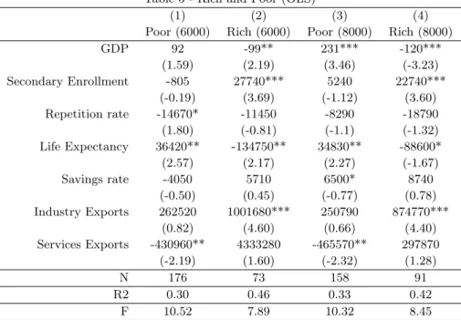
In order to understand the differences that are influencing high-low-tech ratio in poor and richer countries, we have divided the sample, and present the results in Table 5.
Table 5 - Rich and Poor (OLS)
(1) (2) (3) (4)
Poor (6000) Rich (6000) Poor (8000) Rich (8000)
GDP 92 -99** 231*** -120*** (1.59) (2.19) (3.46) (-3.23) Secondary Enrollment -805 27740*** 5240 22740*** (-0.19) (3.69) (-1.12) (3.60) Repetition rate -14670* -11450 -8290 -18790 (1.80) (-0.81) (-1.1) (-1.32) Life Expectancy 36420** -134750** 34830** -88600* (2.57) (2.17) (2.27) (-1.67) Savings rate -4050 5710 6500* 8740 (-0.50) (0.45) (-0.77) (0.78) Industry Exports 262520 1001680*** 250790 874770*** (0.82) (4.60) (0.66) (4.40) Services Exports -430960** 4333280 -465570** 297870 (-2.19) (1.60) (-2.32) (1.28) N 176 73 158 91 R2 0.30 0.46 0.33 0.42 F 10.52 7.89 10.32 8.45
Note: The same definitions as in Table 4. 6000 and 8000 are the threshold values above which a country is rich.
This is an additional robustness test to our specification, by which we can conclude that our main conclusion remains unchanged: high-tech proportion increases in poor countries and decreases in rich countries. The crucial differences between the groups are in the lifetime earnings variable (life expectancy) and in supply (secondary education) and demand of high-techs (services and industry). In fact, in richer countries, we have a negative influence of life expectancy and a positive influence of secondary enrollment and the industry dummy (this last is common to the whole sample). This means that the higher the level of education of population in richer countries and the lower the life expectancy, the higher is the high-low-tech ratio. In poorer countries, however, life expectancy has a crucial and positive influence, as well as the services specialization, with a negative influence. It is well-known that in lower-income countries life expectancy rises more as a country gets richer than in high-income ones. In richer countries the variation of life expectancy between countries is quite low.
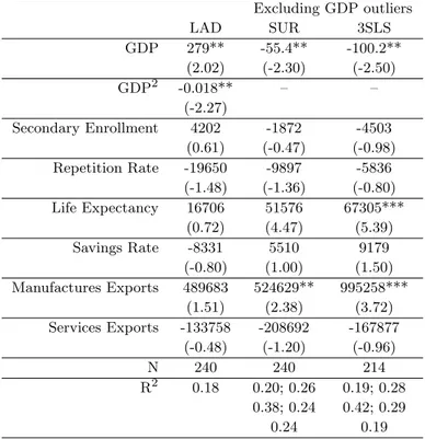
All the main results can be obtained when considering the whole sample (including outliers), although results are omitted for reason of length and simplicity13. The puzzling non-positive
tionship between h/(1 − h) and GDP per capita is well robust to the introduction of a large set of controls, to deletion (or not) of outliers and to possible endogenous variables.
It could be questioned if the possible presence of outliers in GDP (and not only in h/(1 − h)) can affect our results14. These results are presented in Table 2.A, in the appendix A, where it is shown that it is not the case. Also results in section 2 are robust to these exclusion.
4
Conclusion
In the data, high-low-tech ratio has an inverted U-shaped relationship with the level of development, measured as GDP per capita. In fact, we find quite a robust non-positive relationship between high-low-tech ratio and GDP, which reflects that rich countries invest less than lower-income countries in high-tech human capital. This is classified as a stylized fact because it can be seen using different samples (with and without outliers in both dimensions), different periods (each of the five-year periods between 1970 and 199715), different measures (enrollments and graduates) for the proxy for the composition of human capital at universities and colleges. Some additional variables may contribute to explaining the high-low-tech human capital ratio, such as life expectancy and savings rate, which seems to be linked with a greater preference for the future and high lifetime costs of high-tech programs and manufacture exports specialization, which is linked with the demand for the high-tech type of university graduate. Conditional on demand and on the probability of high future earnings, the puzzling relationship of decreasing proportion of high-techs in richer countries remains clear.
There are interesting questions for future research. First, as more data become available, it could be possible to test for productivity and wages micro relationships. Second, a natural research agenda includes fully explaining this puzzling relationship between GDP per capita and the proportion of high-techs in the economy with relation to structural transformation and increasing R&D activity, as the evidence shows a clear relationship between our measure of human capital composition and specialization dummies.
References
[1] Acemoglu, D. (2001), Good jobs versus bad jobs, Journal of Labor Economics, 19(1), pp.1-21, Jan.
[2] Barro, R. and X. Sala-i-Martin (1995), Economic Growth, McGraw-Hill.
[3] Barro, R. (1999), Human Capital and Growth in Cross Country Regression, Swedish Economic Policy Review, number 6.
[4] Barro, R. and J. Lee (2000), International data on educational attainment: upgrades and im-plications, Working Paper n.42, Haward University.
[5] Bertocchi, G. and M. Spagat (1998), The evolution of modern educational systems: technical versus general education, distributional conflict and growth, CEPR Discussion paper 1925. [6] Easterly, W. and M. Sewadeh (2002), Global Development Network Database,
http://www.worldbank.org/research/growth/GDNdata.htm.
14We kept the same definitions of outliers for this case. 15Which indeed, are all the data available.
[7] European Comission (1999), Key data on Education in Europe, Office for Official publications of the European Communities.
[8] Funke, M. and H. Strulik (2000), On Endogenous growth with physical capital, human capital and product variety, European Economic Review, 44, pp.491-515.
[9] Grossman, Gene and Helpman, Elhanan (1991), Innovation and Growth in the global economy, MIT press.
[10] Hayashi, Fumio (2000), Econometrics, Princeton University Press, Oxford.
[11] LaPorta, R. et al. (1998), The quality of government, NBER working paper 6727, September. [12] Murphy, Kevin, Shleifer, Andrei and Vishny, Robert (1991), “The Allocation of talent:
impli-cations for growth”, Quarterly Journal of Economics, May, volume CVI, 2, pp. 503-530. [13] OECD (2002), International mobility of highly skilled, Paris.
[14] Romer, Paul M. (1990), “Endogenous Technological change”, Journal of Political Economy, vol. XCVIII, pp.71-102.
[15] Tavares, J. and R. Wacziarg (2001), “How democracy affects growth”, European Economic Review, 45, pp.1341-1378.
A
Specification Search
Table 1.A. - Determinants of high-low-tech ratio (h/(1 − h)) - OLS - specification search
(1) (2) (3) (4) (5) (6) GDP 139*** 259*** 355 220*** 137*** 180*** (2.66) (5.01) (1.04) (5.42) (5.39) (7.28) GDP2 -0.01*** -0.014*** -0.004*** -0.01*** -0.007*** -0.01*** (-3.11) (-4.24) (-2.94) (-5.64) (-5.31) (-6.46) Secondary Enrolment 9430*** - - - - -(3.84) - - - - -Repetition Rate - -26100*** - - - -- (-3.47) - - - -Life Expectancy - - 37410*** - - -- - (5.56) - - -Savings Rate - - - 8470* - -- - - (1.96) - -Manufactures Exports - - - - 838630*** -- - - - (6.1) -Services Exports - - - 329580*** - - - (-2.95) N 405 284 490 402 499 499 R2 0.16 0.23 0.17 0.14 0.18 0.12 F 26.33 27.68 33.22 21.71 35.24 23.42
Table 2.A. - The possible explanation for high-low-tech ratio Excluding GDP outliers LAD SUR 3SLS GDP 279** -55.4** -100.2** (2.02) (-2.30) (-2.50) GDP2 -0.018** – – (-2.27) Secondary Enrollment 4202 -1872 -4503 (0.61) (-0.47) (-0.98) Repetition Rate -19650 -9897 -5836 (-1.48) (-1.36) (-0.80) Life Expectancy 16706 51576 67305*** (0.72) (4.47) (5.39) Savings Rate -8331 5510 9179 (-0.80) (1.00) (1.50) Manufactures Exports 489683 524629** 995258*** (1.51) (2.38) (3.72) Services Exports -133758 -208692 -167877 (-0.48) (-1.20) (-0.96) N 240 240 214 R2 0.18 0.20; 0.26 0.19; 0.28 0.38; 0.24 0.42; 0.29 0.24 0.19
Notes: t-statistics are heteroskedastic-consistent. Models include an omitted constant.
B
Data description
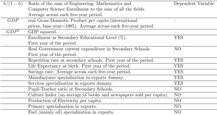
There were three main databases from which we have collected data for this paper: (1) WORLD BANK, Easterly and Sewadeh, Global Development Network Growth Database, from which we collect macroeconomics variables, (2) Barro and Lee database, from which we collect secondary education data and (3) UNESCO database, from which we collect data on enrollments and graduates by tertiary education level by field. The list of countries used in each estimation is available upon request. We present below the list of variables and the result of their submission to the specification test of Table 1.A.
Passed in
Specification Test?
h/(1 − h) Ratio of the sum of Engineering, Mathematics and Dependent Variable
Computer Science Enrollment to the sum of all the fields. Average across each five-year period.
GDP real Gross Domestic Product per capita.(international –
prices, base year=1985). Average across each five-year period.
GDP2 GDP squared. –
Enrollment in Secondary Educational Level (%). YES
First year of the period.
Real Government current expenditure in Secondary Schools. NO First year of the period.
Repetition rate at secondary schools. First year of the period. YES
Life Expectancy at birth. First year of the period. YES
Savings rate. Average across each five-year period. YES
Manufactures specialization in exports dummy. YES
Services specialization in exports dummy. YES
Pupil-Teacher ratio at Secondary Schools. NO
Culture Index (an average of books and newspapers sold per capita). NO
Production of Electricity per capita. NO
Primary specialization in exports. NO
Fuel (mainly oil) specialization in exports. NO
C
Instruments for 2SLS and 3SLS estimation
To select the instruments, we related typically seen exogenous variables with GDP. We selected the significant variables. Then, we performed a comparison between J-statistics in efficient 2SLS (see Hayashi, 2000). First, we show the t-statistics in the regression. Then, a summary of the p-values of the chi-squared statistic we have used.
Table 1.C. - t-statistics Latitude 4.77 Longitude 0.00 Tropical dummy -9.48 Fuel Specialization 1.41 Primary Specialization -0.93 Landlocked -1.81
Black Market Premium -4.63
Ethnoling. Fraccionalization -3.20
R2 0.34; 0.39; 0.48
Table 2.C. - Exogeneity Tests
7579 8084 8589 9094 9597
Latitude 1.4 (0.2) 1.1 (0.3) 0.7 (0.4) 0.5 (0.5) 2.3 (0.1) Tropical dummy 1.6 (0.2) 0.0 (0.8) 0.3 (0.6) 0.7 (0.4) 1.7 (0.2) Black Market Premium 3.0 (0.1) 1.0 (0.3) 0.1 (0.8) 0.5 (0.5) 0.5 (0.5) Ethnoling. Fraccionalization 1.4 (0.2) 0.6 (0.5) 0.8 (0.4) 0.7 (0.4) 0.8 (0.4) Note: This are χ2(1) which tests the null of equal J-statistics. P-values in parentheses.