to factors of production and the elasticity of scale
Adalmir Marquetti
Departamento de Economia, Pontifícia Universidade Católica do Rio Grande do Sul, and Researcher from CNPq, Brazil
Abstract
This paper employs local regression to estimate the output elasticity with respect to labor, human capital, physical capital and the elasticity of scale for 90 countries in 1985 and 1995. The results support the hypotheses of constant returns to scale to factors and decreasing returns to
accumulable factors. The low capital-labor ratio countries have important differences in factor elasticities in relation to other countries. The augmentation of the production function by human capital did not reduce the elasticity of physical capital as suggested by Mankiw, Romer and Weil (1992). Moreover, it is investigated if the factors shares are really equal to their output elasticity. The wage share raises with the capital labor ratio and the sum of the output elasticity of labor and human capital is below the wage share for high capital labor ratio countries, happening the inverse for low capital labor ratio countries. It indicates the presence of externalities, or imperfect competition or that the marginal theory of distribution is inaccurate.
Resumo
Este artigo utiliza regressão local para estimar a elasticidade do produto em relação ao trabalho, cap-ital humano, capcap-ital físico e a elasticidade de escala para 90 países em 1985 e 1995. Os resultados corroboram a hipótese de retorno constante de es-cala. Contudo, os países com reduzida relação capi-tal-trabalho possuem importantes diferenças nas elasticidades dos fatores em relação aos demais países. O aumento da função de produção por capi-tal humano não reduziu a elasticidade do capicapi-tal físico como sugerido por Mankiw, Romer and Weil (1992). Além disso, é investigado se a participação na renda dos fatores de produção é de fato igual à elasticidade do produto. A soma das elasticidades do produto em relação ao trabalho e ao capital humano é menor do que a parcela salarial para os países de elevada relação capital-produto, ocorrendo o contrário nos países de reduzida relação capital-trabalho. Isso indica ou a presença de externali-dades, ou de competição imperfeita ou que a teoria marginal de distribuição é equivocada.
Key words elasticity of output,
elasticity of scale, wage share.
JEL classification O4, C14.
Palavras-chave
elasticidade do produto, elasticidade de escala, parcela salarial.
1_ Introduction
An empirical debate was established between the proponents of the endogenous and exogenous growth theories about the returns to scale to accumulable factors, physical and human capitals and knowledge. In the endogenous growth theories increase in per capita income are explained within the model through the dismissal of the assumption of decreasing returns to scale to accumulable factors, what leads to the rejection of convergence by most of the endogenous growth models. The assumption of decreasing returns to scale to accumulable factors in the exogenous growth theory implies the presence of absolute or conditional convergence in income per capita. Thus, the investigation of returns to capital by estimating the elasticity of output with respect to physical and human capital becomes a line of empirical research.
The direct estimates of the returns to physical capital and the indirect estimates from the velocity of convergence suggested an elasticity of output with respect to physical capital around 0.7. It seems to contradict the marginal productivity theory of distribution that under
competitive markets and constant returns to scale the profit share should be equal to the elasticity of output with respect to physical capital, the profit share in the developed countries is around 0.4. Romer (1987) suggested that the difference is explained by externality in physical capital.
Barro and Sala-i-Martin (1992) argued that it could be explained by the omission of investment in education as part of the accumulable capital. Mankin, Romer and Weil (1992, p. 432) proposed a Cobb-Douglas production function in the form
X = AN1/3H1/3K1/3
The proponents of the endogenous growth models also suggested a broader definition of capital, including other accumulable factors, such as human capital and knowledge. The elasticity of output with respect to the accumulable factors should at least add up to one. In this case the elasticity of scale is greater than one and there is increasing return to scale in the production function.
The aim of this paper is to estimate the elasticity of output with respect to labor, physical capital, and human capital as well as the elasticity of scale. These estimates allow one to answer if the world aggregate
production function presents increasing, constant, or decreasing returns to scale; if the accumulable factors present increasing, constant, or decreasing returns to scale; and, if it is really true that the inclusion of human capital reduces the elasticity of output with respect to physical capital.
We approach these questions employing the non-parametric local regression method (Cleveland, 1993; Loader, 1999). The advantages of this method are that no previous parametric functional form is assumed, no linearity is imposed on the data and it allows for parameter heterogeneity. This
method is based on visualization, which is a powerful mechanism for data analysis and communication, permitting one to observe interesting aspects that are not possible in the parametric framework. For example, it allows observing possible heterogeneity in the output elasticity with respect to factors of production factors and in the elasticity of scale for countries in different states of development. This paper follows Durlauf ’s (2000)
suggestion to employ new econometric techniques to study economic growth.
The evidence will be examined by looking at two data sets for 90 countries in 1985 and 1995 based on, respectively, Summers and Heston (1991) and Heston, Summers and Aten (2002).
2_ Theoretical basis
The theoretical and empirical research in economic growth has experienced a new boom since the second half of the 1980s with the appearance of the endogenous growth theory and data sets in the form of panel data and long-term historical data. In these models the growth in per capita income is explained within the model through the elimination of diminishing returns to capital.
The assumption of diminishing returns to capital implies in the concavity of aggregate production function in Solow-Swan growth model. The concavity of the aggregate production function implies convergence to the steady state. The abandonment of the assumption of diminishing returns leads to the rejection of convergence by most of the EGT literature. Therefore, there was an empirical debate over the returns to capital between the
proponents of the EGT and the defenders of the exogenous growth model. This question has been
investigated mainly with parametric tests assuming previous functional forms and distribution functions.
Kurz and Salvadori (1997) classify the EGT models in three groups of models based on the mechanisms
“embodied” in the aggregate
production function that eliminate the diminishing returns to accumulable factors. The first group represented by Rebelo (1991), King and Rebelo (1990), and Young (1992) assumes constant returns to capital, the AK models. The second group represented by Jones and Manuelli (1990) assumes that
diminishing returns to capital are bounded from below, the combination of an AK with a traditional neoclassical production function. Models in which the aggregate production function might present convex regions represent the third group. This group is split in models with externalities represented by Romer (1986) and Lucas (1988) and in models with scale effects in growth represented by Romer (1990), Grossman and Helpman (1991) and Aghion and Howit (1992).
Cobb-Douglas production function, Romer (1994, p. 6) computed that the savings rate in the U.S. should be from 30 to 100 times greater than in
Philippines for these countries to have a similar growth rate. Moreover, the capital labor ratio in Philippines should be among 0.1 and 0.3% of the capital labor ratio in the U.S. economy to explain the difference in labor
productivity between these countries if they both had access to the same technology. For the Solow-Swan model to explain the differences in labor productivity between these countries the output elasticity with respect to labor should be reduced. In this case, the decreasing returns to capital would happen more slowly.
This result was obtained by Romer (1987). Employing a
Cobb-Douglas with physical capital and labor to describe the production of final goods, he estimated the output elasticity with relation to physical capital between 0.7 and 1. Under the assumptions of perfect competition and constant returns to scale the coefficients of physical capital and labor in the Cobb-Douglas represent, respectively, the share of physical capital and labor. The profit share and wage share in the U.S. correspond approximately
to 1/3 and 2/3. Romer (1987) explained this difference by the externality in physical capital.
King and Levine (1994) also estimated the output elasticity with respect to physical capital and concluded that there are decreasing returns for this factor of production. Therefore, other accumulable factors and technical change must have a relevant role in the determination of the economic growth. The literature on endogenous growth pointed to the importance of human capital and knowledge as fundamental determinants of economic growth.
Similar route was followed by the literature linked to the Solow-Swan model. Barro and Sala-i-Martin (1992) explained the difference between the output elasticity to physical capital and profit share by the omission of investments in education in the production function. Mankiw, Romer and Weil (1992, p. 432) augmented the production function with human capital. The proposed specification assumes the form:
X =(AN)1 – (a+b)HbKa
elasticity with respect to physical capital. This literature argues that this specification is consistent with the results of the empirical studies and it retains the basic presumptions of the Solow-Swan model.
3_ Methodology
In modeling production we follow the simplest neoclassical form of
representing it. We postulate that just one good is produced and technology is represented by an aggregate production function in the form
X = F(N, H, K)
whereXis output;Nis labor;His human capital andKis physical capital.1
The Cambridge capital debate (see Harcourt, 1972) has emphasized the limitations of the macroeconomic measures of capital based on market valuation of the type employed here. That literature, however, suggests that value aggregates carry information about the underlying structure of the capital stock at least for techniques with real wage-profit rate relations that are nearly linear. Ricardo’s conception of the 93% labor theory of value may be interpreted in terms of approximate linearity of the wage-profit rate curve.
No previous specification of the production function is assumed as in the parametric growth literature. For example, Duffy and Papageorgiou (2000) concluded that the aggregated production function for the world economy is a CES instead of a Cobb-Douglas. In fact, both specifications are restrictive (Jorgenson, 1983), imposing strong constraints on the parameters. Thus, they are not capable of accounting for heterogeneity among countries.
The elasticities of output with respect to factors are computed by
e InX
InI
i
i
=¶ 
whereIistands for factori. The
elasticity of scale is equal to the sum of the output elasticities of the factors of production.
Under the assumption of constant returns to scale, the elasticity of scale is equal to one. Moreover, if there is perfect competition in the markets for inputs and output, then the equilibrium occurs in the point where elasticity of output with respect to each factor is equal to its factor share. Under the hypothesis of increasing returns, the elasticity of scale is greater than one. In this case is possible to maintain perfect competition only if there are external
1 We are considering
economies (Romer, 1986; Lucas, 1988). The alternative is to drop the
assumption of perfect competition and consider the case of noncompetitive markets (Romer, 1990). The
endogenous growth models with increasing returns to accumulable factors fall in one of these cases. In the presence of decreasing returns the elasticity of scale is lower than one.
Therefore, this statistical procedure permits one to answer if there are
increasing, constant, or decreasing returns to scale in the production function. Having constant returns to scale it is possible to observe if, as predict by the marginal productivity theory of distribution, the share of each factor is equal to its output elasticity.
Initially we estimate the elasticity of output with respect to factors
considering the production function with labor and physical capital, then we estimate the elasticities in the augmented production function by human capital. The local regression derivatives produce point estimates of the output elasticity with respect to factors for each country in the sample. Then, we employ again local regression to plot the output elasticity of a factor as the y-axis and the ratio between physical capital and labor, k, as the x-axis.
As pointed out by one of the referees, there is a long debate whether the aggregate production function estimates represent an accounting identity or a true production function. The Simon-Shaikh criticism pointed that the estimated parameters of the
aggregated production function using value data capture an underlying accounting identity. It explains the good fits of the aggregate production function and the proximity between the estimated output elasticities and the factor shares.2
Local regression is a
non-parametric method to fit curves and surfaces by smoothing data proposed by Stone (1977), Cleveland (1979), Cleveland, Devlin and Grosse (1988), among others. It has been under considerable interest due to its features and the development of computer power. Loader (1999) presents the latest developments in local regression. The derivative estimate is, in fact, the local slope of the local regression fit. Loader (1999, p. 101) argues that if the local regression fits the data well, then the local slope is a consistent approximation to the derivative. The appendix presents the basic elements involved in the estimation by local regression.
The estimated output elasticities can be compared employing a simple procedure proposed by Bowman and 2 McCombie and Thirlwall
(1994) and Felipe and Fisher (2004) review the
Azzalini (1997, p. 119). It consists in computing the standard error of the difference of the regression curves and, then, superimposing a reference band of two standard errors centered at the average of the two estimated curves. Differences at any capital labor ratio point will be considered where the estimates are separated by more than two standard errors.
Data forXis GDP in 1985 purchasing power parity obtained in Summers and Heston (1991),Kis an estimate of physical capital stock obtained by a perpetual-inventory method following Hulten and Wykoff (1981). The rate of depreciation (d) was calculated with the expression
d = R/T
whereRis the factor that defines the degree of declining balance due to depreciation, andTis the average asset life. The average value found by Hulton and Wycoff (1981) forRis 1.65 for equipment categories, and 0.91 for structure categories. TheRemployed by us is 1.05. It was calculated considering that equipment categories represent 20 percent and structure categories 80 percent of the gross capital formation. The asset life
considered was 20 years, hence the depreciation rate is 5.25 percent.3
Nis the number of workers obtained in Summers and Heston (1991), andHis the stock of human capital. We follow Nehru, Swanson and Dubey (1995) and Duffy and Papageorgiou (2000) defining human capital as
H = MnN
whereMrepresents the mean years of schooling of the labor force. It is obtained in Barro and Lee (2000), being the average schooling years for the population between 25 and 64. Attempts to estimatennon parametrically using physical capital as a proxy for human capital showed that it ranges from minus two to zero forMbetween zero and four years, and from zero to two forMaround ten years. We opt for settingnequal to two, its highest estimated value. It is interesting to observe that Duffy and Papageorgiou (2000, p. 95) also tried to estimaten, “but the estimates were either implausible negative or the iteration procedure failed to converge”. It might be due to the large number of observations with less than four years of average schooling. An important aspect of our results is that the choice ofndid not affect either the
3 The double declining
estimated value of the elasticity of output with respect to physical capital or the sum of the elasticity of output with respect to labor and human capital.
4_ The elasticity of output with respect to factors and the elasticity of scale Figure 1 displays the local regression fit of the smoothed surface between the logarithms of output, physical capital and labor for 1985. The local elasticities of output with respect to factors are estimated from this fitted surface. It is possible to visualize that the log of output tends to rise with log of labor at fixed levels of log of capital; likewise the log of output rises with log of capital at fixed levels of log of labor. The residual plots against each predictor are presented in the bottom two panels to observe the lack of fit or excess smoothing. There is no effect on the diagnostic plots between the residuals and the predictors. The residual plots reveal the presence of outliers; this was handled by the employment of robust local regression in the estimation of the surface.4
Figure 2 displays the local regression fits between the elasticity of output with respect to labor, to physical
capital and the elasticity of scale for the production function in the form X = F(N, K) and the capital-labor ratio and the associated 95%
confidence intervals.5It also presents
the residuals of the elasticity of scale and local regression fit between them and the capital labor ratio in the right bottom panel. It is possible to observe that there is no lack of fit in the estimated elasticity of scale, despite the presence of outliers.6
The hypothesis that there are constant returns to scale in the
production function cannot be rejected, the left bottom panel shows the local regression fit and the 95% confidence interval for the elasticity of scale. The fitted line is around one and the
confidence interval always includes one. The fitted elasticity of output with respect to labor is displayed in the top left panel. It initially presents a sharp fall, from 0.75 to 0.25 for the capital labor ratio between 0 and 10000 1985 PPP. After that, it declines slowly down to 0.22 for the capital labor ratio close to 30000 1985 PPP. Then, it presents a tendency to increase with the capital labor ratio. The output elasticity of labor might be capturing portion of the output elasticity of human capital in the high capital labor ratio countries. 4 Loader (1999, p. 113)
discusses the robust
estimation in local regression.
5 It is possible to classify the
countries in low, below the first quartile, medium-low, between the first quartile and below the median,
medium-high, between the medium and below the third quartile, and high, above the third quartile, capital labor ratio countries. The first quartile is equal to 3638 1985 PPP, the median is 14450 1985 PPP, and the third quartile is equal to 43100 1985 PPP.
6 This was the basic result
12 14 16 18 20 22 24 Log (Base 10) X, 1985 PPP 20 22 18 16 14 Log (Base 10) X,1985 PPP 6 8 10 12 Log(Base 10)X, 1985
workers o o o o o o oo oo o o o o o o o o o o o o o o o o o o o oo o o o o o o oo o o o o o o oo o o o o oo o o oo o o oo o oo o o o o o o o o o o o o o o o oo o o o o o o o o o o o o o o o o o oo o o o o o o o o o o o o o oo o o o o o o o o o o o o o o o oo oo o oo o oo o o o o o o o o o o oo o oo o o ooo oo o o o o o oo o o oo o o o o o o o
6 8 10 12
-1.0 -0.5 0.0 0.5 1.0 Residuals
Log (Base 10) N, workers
-1.0 -0.5 0.0 0.5 1.0 Residuals
14 16 18 20 22
Log (Base 10) N, 1985 PPP Figure 1_ The fitted surface for log(X) = f [log(K), log(N)] and the residual plots
Local robust regression parameters of the fitted surface: bandwidth = 0.48, degree = 2; Local regression parameters of the residuals plots: bandwidth = 0.5, degree = 1. Source: Marquetti (2004).
o o o o o o o o
oooo o o o oo o o o o o oo o o o o o o o o o o o o o o o o o o o o o o o o o oo o o o o o o o o o o o o o o
ooo
o o o o o o o oo o
o oo
oo o o o o o 0.0 0.2 0.4 0.6 0.8 1.0 0.0 0.2 0.4 0.6 0.8 1.0 La bor elasticity Capital elasticity 1.2 1.0 0.8 0.6 0.4 Elasticity of scale 0.2 0.1 0.0 -0.1 -0.2 Residuals of the elasticity of scale
0 20000 40000 60000 80000
K, 1985 PPP
0 20000 40000 60000 80000
K, 1985 PPP
0 20000 40000 60000 80000
K, 1985 PPP
0 20000 40000 60000 80000
K, 1985 PPP (continues from page 104)
Figure 2_ Elasticities of output with respect to factors, the elasticity of scale for the production function in the form X = F(N, K) and the residuals of the elasticity of scale fit
Local robust regression parameters of the labor elasticity: bandwidth = 0.32, degree = 2; Local robust regression parameters of the capital elasticity: bandwidth = 0.34, degree = 2; Local robust regression parameters of the elasticity of scale: bandwidth = 0.30, degree = 2; Local regression parameters of the residual plot: bandwidth = 0.5, degree = 2.
The fitted elasticity of output with respect to physical capital is shown in the top right panel. As can be
observed, there are two segments in the fit. The first segment corresponds to observations of the capital labor ratio between zero and 10000 1985 PPP with the elasticity of output with respect to capital increasing from 0.2 to 0.74. Then, after reaching its maximum in 0.76 for the capital labor ratio close to the medium, it declines slowly until 0.66.7The magnitude
of the elasticity of output with respect to physical capital in the second segment is consistent with most of the empirical literature (Romer, 1987; Mankiw, Romer and Weil, 1992; Wolff, 1991).
This result brings some embarrassment to the neoclassical theory of distribution. The measured elasticity of output with respect to capital in the second segment, between 0.76 and 0.66, is so much higher than the typical capital share in national income for developed countries, between 0.3 and 0.4. The estimated contribution of capital to output is almost twice of the observed profit
share. Capital appears to be paid less than its marginal contribution
to output. The inclusion of intangibles as human and knowledge in the relevant concept of capital, broadening it, was the basic answer of the
neoclassical literature to solve this problem. Nowadays, the broad concept of capital is seen as a major advance in relation to the original Solow-Swan model. However, as we will see, the estimations of the elasticity of output with respect to physical capital are very robust to different specifications of the production function.
Figure 3 displays the elasticity of output with respect to labor, human capital and to physical capital as well as the elasticity of scale for the production functionX = F(N,H,K). The
hypothesis that the elasticity of scale is equal to one cannot be rejected by the 95% confidence interval as can be seen in the bottom right panel of Figure 4. The augmented production function displays constant returns to scale. Moreover, the elasticity of scale presents a slight decrease with the increase in the capital labor ratio.
7 Estimates of the elasticity
0.0
0.2
0.4
0.6
0.8
1.0
La
bor
elasticity
0.0
0.2
0.4
0.6
0.8
1.0
P
hysical
capital
elasticity
0.0
0.2
0.4
0.6
0.8
1.0
Human
capital
elasticity
1.2
1.0
0.8
0.6
0.4
Elasticity
of
scale
0 20000 40000 60000 80000
K, 1985 PPP
0 20000 40000 60000 80000
K, 1985 PPP
0 20000 40000 60000 80000
K, 1985 PPP
0 20000 40000 60000 80000
K, 1985 PPP
Figure 3_ Elasticities of output with respect to inputs and the elasticity of scale for the production function in the form X = F(N, H, K)
The fitted elasticity of output with respect to labor is displayed in the top left panel. It declines rapidly from 0.74 to 0.36 for the labor ratio between 0 and 10000 1985 PPP. Then, the labor elasticity declines slowly as the capital labor ratio increases, reaching 0.1 when the capital labor ratio is around 80000 PPP 1985. The estimated elasticity of output with respect to human capital is presented in the top right panel, it increases as the capital labor ratio rises. The output elasticity of human capital oscillates around 0.04 for the low and medium low capital labor ratio
countries, then it starts to increase in the medium high capital labor ratio
countries, reaching 0.16 at its maximum.8It could indicate some
complementarity between human and physical capital accumulation.
This result is consistent with the Griliches’ (1969) hypothesis of
capital-skill complementarity. It says that physical capital is complementary with human capital. The accumulation of physical capital would raise the elasticity of output with respect to human capital. It is interesting to observe that the capital human elasticity is significantly
0.0
0.2
0.4
0.6
0.8
1.0
Sum
of
labor
and
human
capital
elasticities
0 20000 40000 60000 80000
K, 1985 PPP
0.0
0.2
0.4
0.6
0.8
1.0
Elasticity
of
accumulabre
factures
0 20000 40000 60000 80000
K, 1985 PPP Figure 4_ Elasticity of output with respect to labor and human capital and with respect to accumulable factors
for the production function in the form X = F(N, H, K).
Local robust regression parameters of the sum between labor and human capital elasticities: bandwidth = 0.33, degree = 2; Local robust regression parameters of the elasticity of the accumulable factors: bandwidth = 0.32, degree = 2.
Source: Marquetti (2004).
8 The estimated output
different from zero for countries with capital labor ratio above 10000 1985 PPP, rising with the expansion in capital labor ratio. It also enhances the importance of physical capital
accumulation to foster growth. The fitted elasticity of output with respect to physical capital is shown
in the bottom left panel. There are two segments in the estimated curve. In the first, it raises rapidly from 0.25 to 0.6 for the capital labor ratio between 0 and 8000 1985 PPP. In the second segment, it keeps rising from 0.6 to 0.7. It is interesting to observe that the elasticity of output to physical capital had similar shape and value in the different
specifications of the production function. The augmentation of the production function by human capital does not reduce the estimated elasticity of output with respect to physical capital.9
Figure 4 displays two important elasticities that can be calculated from these estimates, the sum of the output elasticity with respect to labor and human capital and the output elasticity with respect to accumulable factors, human and physical capitals. The left panel presents the former. It has two segments, the first corresponds to observations with capital labor ratio between zero and 8000 1985 PPP with the elasticity declining from 0.8 to 0.4. The second one corresponds to observations of the capital labor ratio above 8000 1985 PPP with the output elasticity falling to 0.25.
The right panel shows the output elasticity with respect to accumulable factors. There are two segments in the
9 The parametric estimates of the production functions
X = f(N,K) andX = f(N,K,H) are displayed below. The augmented production function by human capital did not reduce the physical capital coefficient. Moreover, the estimated
coefficient for human capital is not statistically significant at 10 percent level.
log(X) = 2.86 +0.385log(N) + 0.631log(K) (0.278) (0.033) (0.023)
N= 90,R2= 97.8%, White heteroskedasticity-consistent
standard errors in parenthesis
log(X) = 2.97 + 0.379log(N) + 0.612log(K) + 0.023log(H) (0.314) (0.030) (0.039) (0.024)
N= 90,R2= 98.8%, White heteroskedasticity-consistent
standard errors in parenthesis
The results, as one can see below, are very similar if the outliers are removed from the sample. Thus, the direct estimates of the production function tend to reduce the role of human capital in growth. Pritchett (1996) obtained a similar conclusion.
log(X) = 2.89 + 0.341log(N) + 0.650log(K) (0.201) (0.024) (0.018)
N= 84,R2= 98.7%, White heteroskedasticity-consistent
standard errors in parenthesis.
log(X) = 2.96 + 0.338log(N) + 0.637log(K) + 0.015log(H) (0.280) (0.024) (0.038) (0.038)
N= 84,R2= 98.9%, White heteroskedasticity-consistent
fit. In the first, the elasticity raises rapidly from 0.32 to 0.6 for the capital labor ratio between 0 and 8000 1985 PPP. In the second segment it increases slowly reaching 0.85. An interesting result is that the elasticity of the accumulable factors tended to increase at declining rates. However, the fit does not support the hypothesis of constant returns to accumulable factors postulated by the endogenous growth theory.
It is possible to make comparisons between the estimated output elasticities in the production function with two and three factors. Figure 5 displays the comparisons between the output elasticities of labor and physical capital in the two
specifications of the production function. The left panel shows the output elasticity of labor elasticity in the X =(N,K) and inX =(N,H,K). There are significant differences between them for capital labor ratio above 65000 1985 PPP, but they started to diverge for countries with a capital labor ratio above 25000 1985 PPP. For the high capital labor ratio countries, the output elasticity of labor in the
two-factor production function became significantly larger than in the three factor one, indicating that it could be
picking up some effects of human capital in growth. The comparison between the output elasticity of physical capital inX = F(N,K) and in
X = F(N,H,K) is shown in the right panel. There are significant differences between them just for countries with capital labor ratio around the median. In the other segments of the fits they had similar shape and value.
Thus, the major differences of the output elasticity in the distinct production function specifications are in the output elasticity with respect to labor. In the augmented production function labor elasticity is reduced. Contrarily to Mankiw, Romer and Weil (1992), the consideration of a
production function with labor, human capital, and physical capital as factors of production did not reduce the output elasticity of physical capital.10
Other interesting result is the heterogeneity in the output elasticities in the poorer economies. These countries have a higher labor elasticity and lower capital elasticity than the other countries in the sample.
Durlauf, Kourtellos and Minkin (2001) also found evidence of greater
heterogeneity in the parameters of the poorer economies.
10 It is possible to write the
augmented Cobb-Douglas production function by human capital with constant returns, X = AKa1
Ha2
Na3, in two ways.
First, considering that output is allocated between the
accumulation of physical capital and human capital . In equilibrium the marginal products of physical capital and human capital are equal, thus the production function can be written as
X = A(a
2/a1)
a2Ka1 +a2Na3.
The output elasticity with respect to physical capital is equal toa
1+a2. Therefore, the
addition of human capital should reduce the output elasticity with respect to physical capital. Second, considering that the workers allocate efficiently their time between work and human capital accumulation. In this case, the marginal products of labor and human capital should be equal in equilibrium. The production function can written as
X = A(a
2/a3)
a2Ka1Na2 +a3
. The output elasticity with respect to labor is equal to a
2+a3. The augmentation of
Overall, our results indicate the presence of constant returns to scale in the world production function, decreasing returns to scale in the accumulable factors, and heterogeneity in the output elasticities. Moreover, the addition of human capital reduced the output elasticity of labor, keeping the output elasticity of physical capital unaltered.
5_ Are the factors shares really equal to their marginal contribution to output?
The marginal theory of distribution predicts that under the hypotheses of constant returns and competitive
markets for inputs and output, the factor share is equal to the elasticity of output with respect to that factor. The results support the hypothesis of constant returns to scale, thus it is possible to test if the share of each factor is equal to its output elasticity.
The wage share for 63 countries was computed as the employee compensation in the GDP employing United Nations (1982), United Nations (1989) and United Nations (1994). It was calculated as the average of the available observations for the period 1980-1990. The wage share is not adjusted for self-employment. After adjusting for self-employment, Gollin
k, 1985 PPP
Elasticity
0 20000 40000 60000 80000
0.0
0.2
0.4
0.6
0.8
1.0 Labor elasticity in Y = F(N, K)
References bands
Labor elasticity in Y = F(N, H, K)
k, 1985 PPP
Elasticity
0 20000 40000 60000 80000
0.0
0.2
0.4
0.6
0.8
1.0
Physical capital elasticity in Y = F(N, K)
References bands
Physical capital elasticity in Y = F(N, H, K) Figure 5_ The comparison between the output elasticities in the production with two and three factors
(2002) concluded that the wage share is relatively constant in a cross-section of countries, ranging from 0.65 to 0.80 of GDP.
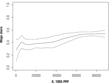
Considering that wage share includes the returns for labor and human capital, then the marginal theory of distribution predicts that the sum of the estimated elasticities of labor and human capital should be equal to the wage share. Figure 6 plots the local regression fit and the 95 percent confidence interval for the capital labor ratio and wage share data.
The local regression fit shows that the wage share tends to increase with the capital-labor ratio. The wage share increases from approximately 30-40 percent in the low capital labor ratio countries to around 55 percent in the high capital labor ratio countries. This result is inconsistent with the conception that a Cobb-Douglas production function describes the world technology. In the Cobb-Douglas the elasticity of substitution is equal to one
and the factor shares are constant.
0 20000 40000 60000 80000
K, 1985 PPP
0.0
0.2
0.4
0.6
0.8
1.0
W
age
share
Figure 6_ The local regression fit and confidence intervals for the relationship between wage share and capital labor ratio
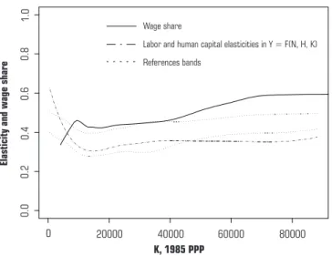
Figure 7 shows the comparison between the sum of output elasticity with respect to labor and human capital and the wage share. It is possible to observe that the wage share is significantly higher than the sum of output elasticity with respect to labor and human capital for high capital labor ratio countries. The opposite happens in the low capital labor ratio countries.11
This result suggests three possibilities. First, there are negative
externalities in physical capital accumulation at low capital labor ratio countries and positive at high capital labor ratio countries. Second, there is imperfect competition that prevents the factors from being paid at their marginal productivity. Third, the marginal theory of distribution is incorrect with labor and human capital being paid above their marginal contribution to output as a condition for technical change as suggested by Foley and Michl (1999, p. 123-127).12
Wage share
References bands
Labor and human capital elasticities in Y = F(N, H, K)
0.0
0.2
0.4
0.6
0.8
1.0
Elasticity
and
wage
share
0 20000 40000 60000 80000
K, 1985 PPP
Figure 7_ Local regression fits and reference bands for comparison between wage share and output elasticity with respect to labor and human capital.
Source: Marquetti (2004).
11 The correction of the
wage share for
self-employment would raise the wage share. The sum of output elasticity with respect to labor and human capital would be lower than the wage share for all levels of the capital labor ratio.
12 Foley and Michl (1999,
6_ Are the results about the elasticities robust?
In this section we investigate if the results about the output elasticities with respect to factors of production and the elasticity of scale are robust to changes in the data set, in the year in analysis, and in the computation of human capital.
The employed data set is based on Heston, Summer and Atti (2002). Data forXis GDP for 1995 measured in 1996 PPP,Kis the stock of physical capital,Nis the number of workers, and His the stock of human capital.
Physical capital is estimated using a depreciation rate of 5.25%. Human capital is computed byH = MnN, where Mis the average schooling years for the population between 25 and 64 years old in Barro and Lee (2000) andnis equal
to one. Despite both samples being of the same size, they are composed by different countries.13
Figure 8 displays the elasticity of output with respect to factors of production, the elasticity of scale and their confidence intervals for the production function in the form X = F(N,K).The elasticities of output with respect to labor and capital and of the elasticity of scale for 1995 are very similar to the estimates for 1985. In particular, two important results are
reproduced. First, the hypothesis of constant return to scale in the
production function cannot be rejected. Second, the low labor ratio countries have a lower elasticity of physical capital and higher elasticity of labor than the other countries. There is heterogeneity in the estimated elasticities of output with respect to factors of production.
Figure 9 presents the elasticity of output with respect to factor of
production and the elasticity of scale for the production function in the form X = F(N,H,K). The results are similar to the estimates for 1985. The
hypothesis of constant returns to scale cannot be rejected by the confidence interval as one can see in the right bottom panel.
The estimated elasticity of output with respect to labor in 1995 declines from 0.6 to 0.3 for countries with low capital labor ratio, keeping constant in 0.2 for countries with capital labor ratio above the medium. The estimated elasticity of output with respect to human capital in 1995 declines from 0.3 to 0 for countries with low capital labor ratio, then it presents a negative segment for countries with capital labor ratio between the first quartile and the medium, rising to approximately 0.2 for countries with high capital labor ratio.
13 The first quartile for the
0.0
0.2
0.4
0.6
0.8
1.0
La
bor
elasticity
0 20000 60000 100000 140000
K, 1996 PPP
0.0
0.2
0.4
0.6
0.8
1.0
Capital
elasticity
0 20000 60000 100000 140000
K, 1996 PPP
0 20000 60000 100000 140000
K, 1996 PPP
1.2
1.0
0.8
0.6
0.4
Elasticity
of
scale
Figure 8_ The estimated elasticity of output with respect to factors of production and the elasticity of scale for the production function in the form X = F(N, K) for 1995
0.0
0.2
0.4
0.6
0.8
1.0
La
bor
elasticity
0 20000 60000 100000 140000
K, 1996 PPP
0.0
0.2
0.4
0.6
0.8
1.0
Physical
capital
elasticity
0 20000 60000 100000 140000
K, 1996 PPP
0.4
0.6
0.8
1.0
1.2
1.4
Elasticity
of
scale
0 20000 60000 100000 140000
K, 1996 PPP
0 20000 60000 100000 140000
K, 1996 PPP
-0.2
0.0
0.2
0.4
0.6
0.8
Elasticity
of
scale
1.0
Figure 9_ The estimated elasticity of output with respect to factors of production and the elasticity of scale for the production function in the form X = F(N, H, K) for 1995
The estimated elasticity of output with respect to physical capital has a similar pattern to previous results. It presents a rising segment from 0.3 to 0.5 for countries with low capital labor ratio, a second segment ranging from 0.6 to 0.75 for the other countries. Another important result is that the augmentation of the production function by human capital did not reduce the elasticity of physical capital. The elasticity of output with respect to labor was reduced in the augmented production function.
Therefore, the results were robust in relation to changes in the data set and the years in analysis. The change in the computation of human capital affects the output elasticity with respect to human capital for countries with capital labor ratio below the average.
7_ Conclusions
The returns to scale to accumulable factors have a central role in the growth literature. In the endogenous growth models it permits continuous growth, while in the Solow-Swan growth model it regulates the speed of convergence to the steady state and the elasticity of output per capital at the steady state with respect to saving. Thus, the growth debate raised an empirical question
about the elasticity of output with respect to accumulable factors.
Initially, the empirical debate centered on the elasticity of output with respect to physical capital. The direct estimations and the indirect estimations through the velocity of convergence suggested an output elasticity of physical capital around 0.7. However, this result is well above the observed profit share in developed countries, which is a serious obstacle for the theory of marginal productivity. The answer for this problem was to reinterpret capital in a broad sense as any accumulable factor, including tangible and intangible capital, so that the estimated output elasticity of accumulable factors and the observed factor shares could be equalized.
This paper employs the
estimated for a cross section of 90 countries in 1985 employing a data set based on Summer and Heston (1991). The robustness of these results were examined looking at data set for 90 countries in 1995 organized from Heston, Summer and Atti (2002).
The estimated elasticity of scale supports the hypothesis of constant returns to scale in the production function. The elasticity of accumulable factors present decreasing returns to scale in the different specifications of the production function. These results are consistent with the Solow-Swan growth models.
The estimated elasticity of output with respect to physical capital is in the range 0.3-0.5 for countries with low labor-capital ratio and 0.6-0.75 for other countries. This result is very robust to different specifications of the production function. The output elasticity of labor is around 0.6 for low capital-labor ratio countries, declining to 0.2 for the countries with high capital-labor ratio. The output elasticity of human capital in 1985 is 0.04 for low capital-labor ratio countries, rising to 0.2 for high capital-labor ratio countries. The low capital-labor ratio countries, which represents the first quartile of the observations, have important parameter differences in relation to other countries.
The augmentation of the production function by human capital did not reduce the elasticity of output with respect to physical capital as suggested by Barro and Sala-i-Martin (1992) and Mankiw, Romer and Weil (1992). The elasticity of output with respect to labor was reduced in the augmented production function.
AGHION, P.; HOWIT, P. Endogenous growth theory. Cambridge, MA: MIT Press, 1992.
BARRO, R.; LEE, J.International
data on educational attainment updates and implications. NBER Working Paper, September, 2000.
BARRO, R.; SALA-I-MARTIN,
X. “Convergence”.Journalof
Political Economy,v. 100, p. 223-251, 1992.
BOWMAN, A.; AZZALINI, A. Applied smoothing techniques for data analysis: the kernel approach with s-plus illustrations. New York: Oxford University Press, 1997.
CLEVELAND, W. Robust locally weighted regression and
smoothing scatterplots.Journal of
the American Statistical Association, v. 74, p. 829-836, 1979.
CLEVELAND, W.Visualizing
data. New Jersey: Hobart Press,
1993.
CLEVELAND, W.; DEVLIN, S. Locally weigthed regression: an approach to regression analysis by
local fitting.Journal of the American
Statistical Association, v. 83, p. 596-610, 1988.
CLEVELAND, W.; DEVLIN, S.; GROASSE, E. Regression by local fitting: methods, properties, and computational algorithms. Journal of Econometrics,v. 37, p. 87-114, 1988.
DUFFY, J.;
PAPAGEOURGIOU, C. A cross-country empirical investigation of the aggregate production function specification. Journal of Economic Growth,v. 5, p. 87-120, March 2000.
DURLAUF, S. Manifesto for a
growth econometrics.Journal of
Econometrics, v. 100, p. 65-69, 2000.
DURLAUF, S.; KOURTELLOS, A.; MINKIN, A. The local solow
growth model.European Economic
Review, v. 45, p. 928-940, 2001.
FAN, J.; GIJBLES, I.Local
polynomial modelling and its applications. New York: Chapman
& Hall, 1996.
FELIPE, J.; FISHER, F. Aggregation in production functions: what applied economists
should know.Metroeconomica, v. 54,
p. 208-262, 2004.
FOLEY, D.; MICHL, T.Growth
and Distribution. Cambridge: Harvard University Press, 1999.
GOLLIN, D. Getting income
shares right.Journal of Political
Ecomomy, v. 110, p. 458-475, 2002.
GROSSMAN, G.; HELPMAN, E.Innovation and growth in the global economy. Cambridge, MA: MIT Press, 1991.
HESTON, A.; SUMMERS, R.;
ATEN, B.Penn World Table 6.1.
Center for International Comparisons at the University of Pennsylvania, 2002.
JONES, L.; MANUELLI, R. A convex model of equilibrium growth: theory and policy
implications.Journal of Political
Economy,v. 98, p. 1008-1038, 1990.
JORGENSON, D. Modeling production for general
equilibrium analysis.Scandinavian
Journal of Economics, v. 85, n. 2, p. 101-112, 1983.
HARCOURT, G.Some cambridge
controversies in the theory of capital. Cambridge: Cambridge University Press, 1972.
HULTEN, C.; WYKOFF, F. The measurement of economics
depreciation. In:Depreciation,
Inflation, and the Taxation of Income from Capital.HULTEN, Charles (Ed.). Washington: Urban Institute Press, 1981.
KING, R.; REBELO, S. Public policy and economic growth: developing neoclassical
implications.Journal of Political
Economy,v. 98, p. 126-150, 1990.
KING, R.; LEVINE, R. Capital fundamentalism, economic development, and economic
growth.Carnegie-Rochester Conference
Series on Public Policy, v. 40, p. 259-292, 1994.
KURZ, H.; SALVADORI, Neri. Theories of ‘endogenous’ growth in historical perspective. In:
TEIXEIRA, J. (Ed.).Money,
Growth, Distribution and Structural Change: Contemporaneous Analysis, Brasília: University of Brasilia Press, 1997.
GRILICHES, Z. Capital–Skill
complementarity.Review of
Economics and Statistics,v. 51, p. 465–468, 1969.
LOADER, C.Local regression and
likelihood. New York: Springer-Verlag, 1999.
LUCAS, R. On the mechanics of economic development. Journal of Monetary Economics, v. 22, p. 3-42, 1988.
MANKIW, N.; ROMER, D.; WEIL, D. A contribution to the empirics of economic growth. Quarterly Journal of Economics, v. 107, n. 2, p. 407-437, 1992.
MARQUETTI, A.Extended Penn
World Tables. Economics Department, New School for Social Research, New York, 2004.
MCCOMBIE, J.; THIRWALL, A. Economic growth and the balance of payments constraint. New York: St. Martins Press, 1994.
NEHRU, V.; SWANSON, E.; DUBEY, A. A new database on human capital stock in developing and industrial countries: sources,
methodology, and results.Journal
of Development Economics, v. 46, p. 379-401, 1995.
OECD.Measuring Capital OECD
Manual: Measurement of Capital Stocks, Consumption of Fixed Capital and Capital Services.Paris: OECD. 2001.
PRITCHETT, L. Where has all the education gone? World Bank Policy Research Working Paper n. 1581, 1996.
REBELO, S. Long-run policy analysis and long-run growth. Journal of Political Economy, v. 99, p. 500-521, 1991.
ROMER, P. Increasing returns
and long-run growth.Journal of
Political Economy, v. 94, n. 5, p. 1002-1037, 1986.
ROMER, P. Crazy explanations for the productivity slowdown. NBER Macroeconomics Annual, v. 2, p. 163-210, 1987.
ROMER, P. Endogenous
technological change.Journal of
Political Economy, v. 98, S71-S10, 1990.
ROMER, P. The Origins of Endogenous Growth. Journal of Economic Perspectives, v. 8, p. 3-22, 1994.
STONE, C. Consistent nonparametric regression, with
discussion.The annals of statistics,
v. 5, p. 549-645, 1977.
SUMMERS, R.; HESTON, A. The penn world table (Mark 5): an expanded set of international comparisons, 1950-1988. Quarterly Journal of Economics, 106: 327-368, 1991.
HESTON, A.; SUMMERS, R.;
ATEN, B.Penn World Table 6.1.
Center for International Comparisons at the University of Pennsylvania, 2002.
UNITED NATIONS.Yearbook
of national accounts statistics 1980: International Tables, vol. II, New York. 1982.
UNITED NATIONS.National
accounts statistics: analysis of main aggregates, 1986. New York, 1989.
UNITED NATIONS.National
accounts statistics: main aggregates and detailed tables, 1992. New York, 1994.
YOUNG, A. A tale of two cities: factor accumulation and technical change in Hong Kong and Singapure. In: BLANCHARD, Olivier; FISCHER, Stanley (Eds.). NBER Macroeconomics Annual 1992, Cambridge: MIT Press, 1992.
WOLFF, E. Capital formation and productivity convergence
over the long term.American
Economic Review, v. 81, p. 565-579, 1991.
WOLFF, E. Capital formation and productivity convergence
over the long term.American
Economic Review,v. 81, p. 565-579, 1994.
I would like to thank Duncan Foley, Duílio Bêrni, and two anonymous referees for very helpful observations on an earlier version of this paper. All remaining errors are mine. Financial support was provided by CNPq.
Author’s e-mail: [email protected]
Local regression is
non-parametric method that employs smoothing to fit curves and surfaces. The basic ideas of the method can be expressed considering the model:
yi=f(x1i,x2i, ...,xip) +e
i,i= 1, ...,n
whereyiis the dependent variable and
xipare thepindependent variables, and
e
i are the errors that are assumed to be normally and independently distributed with mean 0 and constant variance,s2.
The goal is to estimate the regression function f directly without references to a previous functional form.
Local regression estimates the functionf at a valuexin the
p-dimensional space employing weighted least squares. This estimation is obtained defining a neighborhood in the space of independent variables which comprises a subset of
observations that are closest tox. The neighborhood size is defined by the bandwidth,k, with 0 <k £1. The
bandwidth indicates the proportion of
points of the total observations that are considered in the computation of the smoothed function. It controls the smoothness of the fit. Generalized Cross Validation and Akaike’s
Information Criterion were used in the bandwidth definition.
The bandwidth defines a neighborhood in the space of
independent variables, the points in this space are weighted according to their distance tox. The points closest tox have large weight, the points far fromx have lower weight. The weight function employed in the estimates in this paper was the gaussian function. Moreover, it is necessary to choose the degree of the polynomial of the independent variables that is fitted to the dependent variable. In the applications in this paper the degree is equal to one or two. The degree of fit was chosen by a series of local regression plots according to the recommendations by Loader (1999). This procedure defines the value of the estimated function at x. It is repeated
for each point of interest to obtain the estimated function.
Loader (1999) and Cleveland and Devlin (1998) suggest a series of graphs to check the assumptions of normality and constant variance of the residuals. The observation of these figures suggested that the residuals were homocedastic.
The statistical properties of local regression have been studied, allowing to calculate confidence intervals and to realize tests of
hypothesis. Cleveland and Devlin (1988) and Fan and Gijbels (1996) present the basic conception of the statistical inference in local regression. The confidence intervals in the paper are computed locally, pointwise confidence interval. Loader (1999) discusses the difference between pointwise and simultaneous confidence intervals.
Considering that local regression provides a reasonable fit to the data in the smoothing window, then local regression slope provides a good estimation of the derivative (Loader, 1999, p. 101). The degree of polynomial should be at least of order one greater than the derivative that will be
estimated. It is important to consider that the derivative estimation is the