Characterization of a pediatric rotary blood pump

DOI: https://doi.org/10.1590/2446-4740.180046 Volume , Number , p. ,

Introduction

Ventricular assist devices are an important and increasingly prevalent treatment for adult and pediatric patients exhibiting advanced heart failure. These devices can be used as a bridge to heart transplant or destination therapy, and they are classified according to the pumping principle as volume-displacement (pulsatile-) or continuous-flow pumps (RBPs) (Stanfield and Selzman, 2013).

The evolution of VADs from pulsatile pumps to rotary blood pumps has started a new era for the treatment of heart failures. The RBP provides a continuous flow of

blood for the patient and the increase of its clinical usage comes from their smaller size, improved durability and increased survival with less morbidity when compared to the performance of pulsatile pumps (Moazami et al., 2013).

Typical impeller types for RBPs, such as axial or centrifugal pumps, are designed to operate around a specific speed, pressure, and flow. Classically, axial-flow pumps tend to be used for high flow rates and low-pressure head conditions, whereas centrifugal-flow ones are designed for low flow rates and high-pressure head conditions (Stanfield et al., 2012).

For the development of the physiological control system, the steady-state and dynamic operation of RBPs must be investigated. Within the model-based design framework, rotary blood pumps used as VADs are usually represented by lumped parameter models, named as 0D models (Capoccia, 2015; Moscato et al., 2009). This type of model is the most adopted because it uses a relatively small number of parameters to simulate the cardiovascular hemodynamics. Besides, the concept of analog circuitry is used, in which the electric current represents the fluid flow in the blood vessels, and the electrical voltage represents the pressures in the circulatory system (Shi et al., 2011).

Characterization of a pediatric rotary blood pump

Thamiles Rodrigues de Melo

1

_{, Felipe José de Sousa Vasconcelos}

1

_{, Luiz Henrique Ramalho Diniz Ribeiro}

2

_,

Simão Bacht

3

, Idágene Aparecida Cestari

3

_{, José Sérgio da Rocha Neto}

1

_{, Antonio Marcus Nogueira Lima}

1

_*

1 _{Graduate Program in Electrical Engineering, Federal University of Campina Grande, Campina Grande, PB, Brazil.}

2 _{Undergraduate Program in Electrical Engineering, Federal University of Campina Grande, Campina Grande, PB, Brazil.} 3 _{Bioengineering Division, Heart Institute, São Paulo, SP, Brazil.}

Abstract Introduction: A ventricular assist device (VAD) is an electromechanical pump used to treat heart failures. For designing the physiological control system for a VAD, one needs a mathematical model and its related parameters. This paper presents a characterization procedure for determining the model parameter values of the electrical, mechanical, and hydraulic subsystems of a pediatric Rotary Blood Pump (pRBP). Methods: An in vitro test setup consisting of a pRBP prototype, a motor driver module, an acrylic reservoir, mechanical resistance and tubings, pressure and

fluid flow sensors, and data acquisition, processing, and visualization system. The proposed procedure requires

a set of experimental tests, and a parameter estimation algorithm for determining the model parameters values.

Results: The operating limits of the pRBP were identified from the steady-state data. The relationship between the

pressure head, flow rate, and the rotational speed of the pRBP was found from the static tests. For the electrical and mechanical subsystems, the dc motor model has a viscous friction coefficient that varies nonlinearly with the flow. For the hydraulic subsystem, the pressure head is assumed to be a sum of terms related to the resistance, the inertance, the friction coefficient, and the pump speed. Conclusion: The proposed methodology was successfully

applied to the characterization of the pRBP. The combined use of static and dynamic tests provided a precise lumped

parameter model for representing the pRBP dynamics. The agreement, regarding mean squared deviation, between

experimental and simulated results demonstrates the correctness and feasibility of the characterization procedure.

Keywords Rotary blood pump, Ventricular assist device, Centrifugal flow pump, Lumped parameter model, System identification.

This is an Open Access article distributed under the terms of

the Creative Commons Attribution License, which permits

unrestricted use, distribution, and reproduction in any medium,

provided the original work is properly cited.

How to cite this article: Melo TR, Vasconcelos FJS, Ribeiro LHRD,

Bacht S, Cestari IA, Rocha Neto JS, Lima AMN. Characterization

of a pediatric rotary blood pump. Res Biomed Eng.  ;   : . DOI:

10.1590//2446-4740.180046

*Corresponding author: Graduate Program in Electrical

Engineering, Federal University of Campina Grande, Rua Aprigio Veloso, 882, CEP 58429-900, Campina Grande, PB, Brazil.

E-mail: amnlima@dee.ufcg.edu.br

The objectives of this paper are to obtain the lumped parameter model and to present a characterization procedure for a pediatric rotary blood pump (pRBP) prototype.

Methods

This section describes the in vitro experimental test setup configuration, the dynamic equations used for representing the behavior of the electrical, mechanical and hydraulic subsystems, and the proposed characterization procedure for pRBP.

In vitro experimental test setup

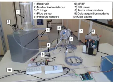
The in vitro experimental test setup used to characterize

the pRBP is shown in Figure 1. This test setup consists

of: a rotary blood pump prototype, a motor driver module, pressure and fluid flow sensors, data acquisition boards, an acrylic reservoir, a mechanical resistance, and

tubings. A computer (not shown) running the Microsoft Windows operating system provides the data processing and data visualization. A USB interface provides the data transmission from the test setup to the computer. The structure of the experimental test setup is relatively simple to build and allows to put the pRBP to operate at different pressures and fluid flow levels.

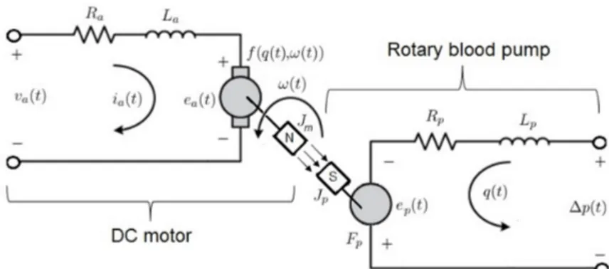
Figure 2 shows a simplified block diagram to explain the coupling of the electrical, mechanical and hydraulic subsystems. The dc motor is the actuator of the electrical subsystem, in which the motor driver module provides the armature voltage. The pump is connected to the reservoir, the pressures and flow may be measured at the inlet and outlet of the pump. It is worth to point out that this type of test setup structure is widely used in RBPs characterization (Ganushchak et al., 2006;

Jahanmir et al., 2008; Pennings et al., 2013).

In the hydraulic subsystem, the pRBP (20 mL ejection volume) is a centrifugal rotary blood pump to be used

Figure 1. Photograph of the in vitro experimental test setup. The parts identification and description are provided in the white box.

as a bedside pump for the patient. In the mechanical subsystem, there is a coupling between the pRBP and the dc motor shaft. The two parts of the coupler, one at dc motor side and the other at the impeller side have four permanent magnets.

The coupling between the motor shaft and the RBP impeller is magnetic since it causes less friction with blood; thus heat generation is minimized, and therefore, less formation of thrombi and occurrence of hemolysis (Pérez, 2009). In this type of pump, the blood flow is generated by the impeller rotational speed. The impeller is enclosed in a polycarbonate housing with central access inlet connector and peripheral access outlet connector.

The rotary pump inlet and outlet accesses are connected to an acrylic reservoir using tubings. The liquid used in the tests is a solution composed of 2 / 3 saline solution and

1 /3 glycerin designed to reproduce the blood viscosity. Additionally, there is a mechanical resistance which changes the cross-section of the tubing to simulate obstructions. The test setup is equipped with sensors that allow the measurement of the pressure head ∆p t

( )

(the pressure

difference between the pump outlet (pout( )t) and pump

inlet (pin

( )

t)), the fluid flow at the outlet tubing q t

( )

,

the motor armature voltage v_a

( )

t , the armature current

( )

a

i t, and the mechanical shaft speed ω

( )

t . The pressure signal is measured with a TruWave disposable pressure transducer (Model number PXMK2051), which is based on the principle of strain-gauge and operates in the pressure range from -50 to +300 mmHg (Edwards Lifesciences Corporation, 2018). The fluid flow is measured with a em-tec Digiflow-EXT1 non-invasive flow sensor (Model number 2017103945), using ultrasound scheme with Clamp-On Transducer CT 1/4” x 1/16” and operates

in the flow range ±32 L/min (Germany em-tec GmbH,

2018). The rotational speed is measured by using a 15-hole encoder installed at the dc motor side of the magnetic coupler. The analog signals provided by these sensors are acquired by using National Instruments boards

(NI USB-6210 and NI myDAQ) and delivered to the computer via the USB interface. These boards allow both single and multiple 16-bit analog-digital conversions. To avoid data loss during the experimental tests a large first-in-first-out buffer is provided. The setup also has software for selecting the structure of the mechanical and hydrodynamic dynamics, and for estimating all the model parameters; the software runs on a desktop

computer not shown in Figure 2.

Pump modeling

The lumped parameter model for the pRBP prototype system is described by a set of three ordinary differential equations. The equivalent circuit representation for this

lumped parameter model is as shown in Figure 3.

The electrical subsystem is composed of a dc motor. The differential equation for this subsystem is found by applying the Kirchhoff’s voltage law to the armature circuit. Thus, the model for the electrical subsystem is given by

( )

1

_{( )}

_{( )}

_{( )}

,a a e

a a

a a a

di t R k

v t i t t

dt =L −L −L ω (1)

where Ra is the armature resistance, La is the armature

inductance, ke is the back-emf constant, ea

( )

t is back-emf

voltage, and ω

( )

t is the rotor speed, in which e ta

( )

= ωke

( )

t.

For the mechanical dynamics, the difference of the electromagnetic torque and pump torque determines the energy used for accelerating or decelerating the impeller. There is an axial-type magnetic coupler between the dc motor and the pump impeller. Permanent magnets are disposed on a disk fixed at the dc motor shaft spinning

with rotational speed ωm. At the pump impeller side,

the magnets are disposed over a polycarbonate disk

rotating with rotational speed ωp (Lubin et al., 2014).

In this paper, for simplicity, we assume that the coupler

is rigid, i.e., ωm( )t = ωp( )t = ω( )t , and thus the motion

equation is given by

( ) _{( )}

,m e l

d t

J c t T T

dt

ω

− ω = − (2)

where Jm is the moment of inertia, c is the viscous

friction coefficient, Te is the electromagnetic torque, given

by Te=k ie a

( )

t, and Tl is the load torque (pump torque).

Defining f q t( ( ) ( ),ωt )= ωc ( )t +Tl as the net pump torque

one may rewrite the motion equations as

( )

_{( )}

1

₍

_{( ) ( )}

₎

,e

a

m m

d t k

i t f q t t

dt J J

ω

= − ω . (3)

The reason for writing the motion equation like this is related with the fact that the expression for

( ) ( )

( , )

f q t ω t is not known a priori, and must be defined in the characterization procedure. The pump torque acting on the dc motor shaft depends on the type of coupling device and on how the impeller blades interact with the flow. In this paper, we consider that f q t( ( ) ( ),ω t ) is one

out of the five possible structures given below

( ) ( )

( ) ( )

Model I : f q t ,ωt = ωc t , (4)

( ) ( )

(

)

2

( )

( )

Model II : f q t ,ω t =_aq t + ωc_ t , (5)

( ) ( )

(

)

2

( )

( )

( ) ( )

2

Model III : f q t ,ωt =_aq t + ω +c_ t bq t ω t , (6)

( ) ( )

(

)

2

( )

( )

3

( )

Model IV : f q t ,ωt =_aq t + ω + ωc_ t d t , (7)

( ) ( )

(

)

2( ) ( ) ( ) ( )2 3( )

Model V : f q t ,ωt =_aq t + ω +c_ t bq t ω t + ωd t . (8)

In Model I, the function f q t( ( ) ( ),ω t ) is dependent only on the linear component of the viscous friction (c) generated by the dc motor. In Model II, a

non-linear term quadratic (a) with the flow is added to the constant viscous friction coefficient. In Model III, a bi-linear term (b) involving the flow multiplied by the square of the rotational speed is included. In Model IV, the bi-linear term is replaced by one that depends on the cube of the rotational speed (d). In Model V, all the previous terms are combined (Choi et al., 1997;

Lim et al., 2007).

For the hydraulic dynamics, the pressure head, fluid flow, and rotational speed relationship can be described by using Euler’s pump and turbine equations. However, there is no simple theoretical method for finding this relationship without using finite element analysis. Thus, similarly to what was said for the motion equation, the function that relates the pressure head with fluid flow

and rotational speed is not known a priori and also must

be defined in the characterization procedure. In this

paper, we consider that ∆p t

( )

is one of the five possible

models given below

( ) ( ) 2( )

Model I : ∆p t =R q tp + βω t , (9)

( ) ( ) 2( ) 2( )

Model II : ∆p t =R q tp +F qp t + βω t , (10)

( ) ( ) 2( ) 2( ) ( )

Model III : p p p ,

d t

p t R q t F q t t J

dt

ω ∆ = + + βω + (11)

( ) ( ) 2( ) 2( ) ( )

Model IV : p p p ,

dq t

p t R q t F q t t L

dt

∆ = + + βω + (12)

( ) ( ) 2( ) 2( ) ( ) ( )

Model V : p p p p .

dq t d t

p t R q t F q t t L J

dt dt

ω ∆ = + + βω + + (13)

In Model I, the pressure head is assumed to be a sum of a term proportional to the flow (related to the pump resistance Rp), and a nonlinear term quadratic with the

rotational speed (β), in which ( ) 2( ) p

e t = βω t . In Model II, non-linear term quadratic (Fp) with the flow is added.

In Model III, a term proportional to the time derivative of the rotational speed (related to the impeller pump’s moment of inertia Jp) is included. In Model IV, the term

proportional to the time derivative of the rotational speed is replaced by one proportional to the time derivative of

the flow (related to the pump’s inertance Lp). In Model

V, all the previous terms are combined (Pirbodaghi et al.,

2011; Pirbodaghi, 2017; Zhang et al., 2010).

As mentioned before, the selection of the structure for the mechanical and hydrodynamic dynamics, and the estimation of all the model parameters is provided by a software. Thus, the continuous-time models used for representing the electrical, mechanical and hydraulic subsystems must be converted into discrete difference equations, suitable for numerical computing. Among the several methods for deriving the discrete-time representation (Santina and Stubberud, 2010), in this paper, for simplicity, the forward Euler method was used, i.e., dx t( ) x t( t) x t( )

dt t

+ ∆ − ≈

∆ , where x t

( )

may represent

( )

a

i t , ω

( )

t, q t

( )

. Applying forward Euler method to the

electrical, mechanical and hydraulic subsystems models the following discrete-time representations are obtained

( ) ( ) ( ) 2 ( )

1 1 a e ,

a a a

a a a

hR h hk

i k i k v k k

L L L

 

+ = −  + − ω

  (14)

( ₁) ₁ ( ) e ( ) 2( ) ( ) ( ) ( )2 3( )_,

a

m m m m m

hk

hc ha hb hd

k k i k q k k q k k k

J J J J J

 

ω + = − ω + − ω − ω − ω

  (15)

( ₁) ₁ p ( ) p 2( ) 2( ) ( ) p ( ₁) ( )_,

p p p p p

hR hF h h J

q k q k q k k p k k k

L L L L L

  β

+ =_− _ − − ω + ∆ − ω + − ω  (16)

where k=1, ,N, with N is the number of data samples

mechanical and hydraulic models, we only show the equations for the fifth cases (Model V), since from these expressions one may derive the other representations (Models I-IV) just by deleting the terms not being used.

Pump characterization procedure

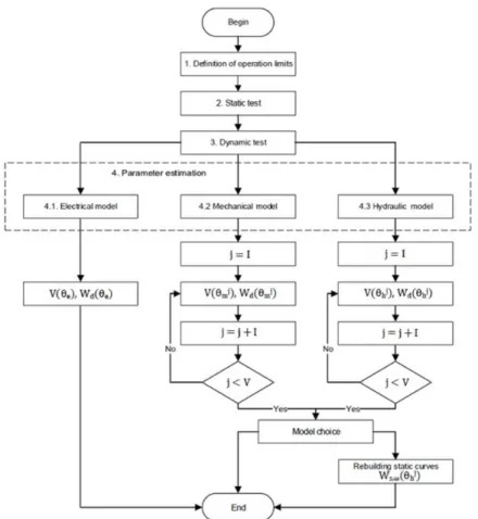
The selection of the structure for the mechanical and hydrodynamic dynamics and the estimation of all the model parameters of the pRBP is based on a sequence of experimental tests and a numerical algorithm. The proposed characterization procedure for this purpose is sketched in the flowchart of Figure 4. In the following a detailed explanation of all steps of the characterization procedure will be provided.

Definition of operating limits

An initial test using the pRBP is executed for defining the operating limits, regarding the maximum and minimum values of the signals available on the in vitro experimental setup. This step is performed as follows:

a) With the mechanical resistance fully open (see

tag 2 at Figure 1), the armature voltage (see v_a

( )

t at Figure 2) is changed from 0 V to the maximum voltage provided by motor driver module in steps of 1 V at a time; at each step the voltage level is kept constant for 1 min;

b) After 1 min, when the steady-state is reached, the armature voltage, the armature current, the rotational speed, the fluid flow and the pressures (at the pump inlet and pump outlet) are recorded;

c) Repeat (a) and (b) until the magnetic coupler decouples the motor shaft from the pump. The decoupling is detected by a sudden reduction of the armature current, rotational speed, and fluid flow.

Static test

The traditional method for characterization of rotary pumps consists in generating pressure head x flow plots, i.e., ∆ ×p q curves (Ganushchak et al., 2006). In this method, the flow rate, and the pressure head at different rotational speeds, under steady-state conditions,

are recorded. The procedure to obtain hydrodynamic performance is as follows:

i. In the motor driver module, the pump speed is changed from minimum speed (the value that guarantees the complete circulation of fluid in the experimental setup) to the maximum speed (the value that allows pumping without to sink the flow during the tubing obstruction) by applying a 500 RPM step.

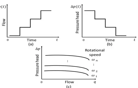
ii. For each rotational speed, the flow is changed in steps of 1 L/min and maintaining each step for 1 min based on the mechanical resistance, from

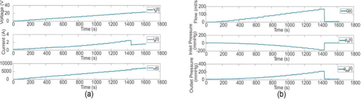
fully closed to fully open as shown in Figure 5a.

iii. After stabilizing the flow at each step, the inlet and outlet pump pressures are recorded as shown in Figure 5b. At the end of the test, ∆ ×p q curves are plotted with the measured values, as shown in Figure 5c.

Dynamic test

To select the structure for the mechanical and hydrodynamic dynamics and to estimate all the pRBP model parameters, a dynamic test is done on the in vitro experimental test setup based on operating limits already found. The procedure used for this test is as follows:

i. With the mechanical resistance fully open, a variable frequency voltage signal is applied to the armature of dc motor for 1 min.

ii. During this 1 min, the armature voltage, the armature current, the rotational speed, the flow and the inlet/outlet pressures are recorded. At the end of the test, the recorded data is split into two parts, one for parameter estimation and another part for model validation.

Parameter estimation

Based on the discrete-time models given by Equations 14, 15 and 16 one may derive one-step-ahead predictors for formulating the parameter estimation problems (Ljung, 1987). For this purpose the discrete-time models must be rewritten as

( )

( | )

ˆ T

i i

y k θ = ϕ k θ . (17)

Based on NE

i

Z , the experimental data matrix recorded during the dynamic test, a cost function

(

, NE

)

i i

V θ Z is defined. The cost function is expressed by

(

)

( ) ( ) { }

1

2 1

, E E ˆ | , e, m, h ,

N N

i i i i

k E

V Z y k y k i

N =

θ = ∑_ − θ _ ∈ (18)

where NE is the number of data points selected for

parameter estimation, i denotes the electrical (e),

mechanical (m) or hydraulic (h) discrete-time subsystem model. The parameter estimate for each subsystem model is found with a numerical algorithm designed to solve (Ljung, 1987)

(

)

{ }

argmin , , e, m, h

ˆ E

i

N

i V i Zi i

θ

θ = θ ∈ _{. (19)}

Model validation

For determining the quality of the estimated model, the part of the data matrix not used in Equation 19 is used to compute a figure of merit, the root mean square error (RMSE) index. This figure of merit indicates the accuracy of the estimated model.

(

)

( )

( )

{ } { }

1

2

1

ˆ, V V ˆ |ˆ , e, m, h , I, II, III, IV,V,

N N

j j

d i i i i

k V

W Z y k y k i j N =

 

∑  

θ = − θ ∈ ∈ (20)

where NV =N−NE.

The block named “Model choice” (see Figure 4) is implemented by using the above figure of merit. Once all the parameters of all models (Models I-V for the mechanical and for the hydraulic subsystems) are available, one computes

( )

ˆ

{

( )

ˆI ,

( )

ˆII ,

( )

ˆIII ,

( )

ˆIV ,

( )

ˆV

}

dθ =m Wdθm Wd θm Wd θm Wd θm Wdθm



and ( )ˆ

{

( )ˆI , ( )ˆII, ( )ˆIII , ( )ˆIV , ( )ˆV

}

dθ =h Wdθh Wdθh Wdθh Wdθh Wdθh

 and look for

the model exhibiting the lowest

( )

ˆj, { } {m, h , I, II, III, IV, V} d i

W θ i∈ j∈ .

Rebuilding of static curves

An additional step, usually not considered in parameter estimation problems is introduced in the proposed characterization procedure. This additional step consists in using the model issued form the parameter estimation algorithm to simulate the static test and compare the simulated results with the actual data recorded previously. The final quality of the model is defined regarding another figure of merit. This figure of merit is expressed by

( ) ( ) ( )2 [ ] { }

, 1

1

ˆ 1 ˆ ˆ

j M |j , , , I, II, III, IV, V ,

s h s s h n

k

W q k q k j

M

ω

=

 

∑ 

θ = − θ _ ω∈ ω ω ∈ (21)

where M is the number of data points recorded in the

static test, q ks

( )

is the actual fluid flow measurement,

and ˆ ( | ˆ )

i

s h

q k θ is the simulated fluid flow computed

with estimated parameter set at the same operating conditions of the static test. This figure of merit is like a cross-validation procedure that corroborates the correctness of the proposed approach specifically regarding the hydrodynamic behavior.

Results

In this section, the data collected at the three first steps of the proposed characterization procedure are presented, compared and discussed.

Operating limits

From the measurements collected at the in vitro experimental setup, the operating limits of the pRBP were defined. In this case, the voltage applied to the armature of the dc motor can keep the pump in full operation up to 21 V, with the current saturating at 2 A and the rotational speed around 6000 RPM, as can be seen in Figure 6a. After this operating point, the flow, and the inlet/outlet pressures goes to zero; this fact is an indication that there is an uncoupling between dc motor and the pump impeller, as can be seen in Figure 6b.

Static test

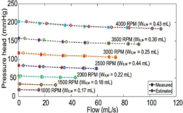
After defining the operating range, the static test was done using the pRBP. In this work, the minimum rotational speed for start pumping is 1000 RPM, whereas the maximum rotational speed, with the mechanical resistance fully closed, is 4000 RPM; above that value, the pump collapses. Thus, in all the subsequent tests the pump speed was restricted to the interval [1000,4000] RPM. Figure 7 shows the plots of q t

( )

×t and ∆p t

( )

×t as obtained in one of the static tests. From the signals recorded in all the static tests, the performance curves

were plotted as shown in Figure 8.

Figure 6. Definition of the pump operating limits for: (a) electrical and mechanical quantities; (b) hydraulic quantities.

Dynamic test

The dynamic test provides the measurements of armature voltage, stator current, flow, pressure head and rotational speed available on the experimental test setup to be used in the parameter estimation and validation tasks. As mentioned before the experimentally collect data are split into two parts. Eighty percent of data were used for parameter estimation, whereas twenty percent of them were used for model validation. In both cases, the units of measurement of flow and rotational speed were converted to standard units, i.e., ml/s and rad/s, respectively.

For estimating the discrete-time subsystems model parameters, the extended recursive least squares (ERLS) algorithm (Åström and Wittenmark, 1994; Chen, 2004) was used; it allows one to estimate numerical values for Ra, La, ke, Jm, a, b, c, d, Rp, Fp, β, Lp and Jp. In this

algorithm, the model is considered as a stochastic system, wherein each differential equation is rewritten as a autoregressive-moving average with exogenous terms (ARMAX) process (Ljung, 1987), according in Equation (22).

( ) ( )

( ) ( )

( ) ( )

,A q y k =B q u k +C q e k (22)

where y k

( )

is the model output, u k

( )

is the model input,

( )

e k is the system noise, ( ) 1

1

1 ... a

a

n n A q = +a q− + +a q− ,

( ) 1

1 ... b b

n n

B q =b q− + +b q− and ( ) 1 1 1 ... c c

n n C q = +c q− + +c q− are

the polynomials in the forward shift operator q, with

orders n_a, n_b and n_c, respectively. The ARMAX model cannot be converted directly to a regression model, since the noise variables e t

( )

are not known a priori. Thus, to derive a regression model suitable approximation, in which the noise is approximated by the residual vector

( )

k

ε , as expressed in Equation (23).

( )_{k y k}( ) T( ) ( )_k ˆ _{k ,}

ε = − ϕ θ (23)

where [1 ... a ... 1 b ... 1 c] T

n n n

a a b b c c

θ =

is the parameters vector and

( ) ( 1 ... ) ( ) ( 1 ... ) ( ) ( 1 ... ) ( )

T _{k y k y k n u k u k n k k n}

ϕ = −_ − − − − − ε − ε − _

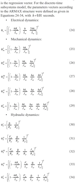
is the regression vector. For the discrete-time subsystems model, the parameters vectors according to the ARMAX structure were defined as given in

Equations 24-34, with h=0.01 seconds.

• Electrical dynamics:

2 1

T

a e

e

a a a

hR h hk

L L L

  

θ = −  

  

  (24)

• Mechanical dynamics:

1 T I e m m m hk hc J J   

θ = −  

  

  (25)

1

T

II e

m

m m m

hk

hc ha

J J J

  

θ = −  

  

  (26)

1

T

III e

m

m m m m

hk

hc ha hb

J J J J

  

θ = −  

     (27) 1 T IV e m

m m m m

hk

hc ha hd

J J J J

  

θ = −  

     (28) 1 T V e m

m m m m m

hk

hc ha hb hd

J J J J J

  

θ = −  

  

 

(29)

• Hydraulic dynamics:

1 T I h p p R R

β 

θ =  

 

  (30)

1 T p II h

p p p

F

R R R

 β 

θ =  

 

  (31)

1 T p p III h

p p p p

F J

R R R R

 β 

θ =  

 

  (32)

1 1 T p p IV h

p p p p

hR F

L L L L

  β 

θ =_ − _ 

_{ }    (33) 1 1 T

p p p

V h

p p p p p

hR F J

L L L L L

  β 

θ =_ − _ 

  

 

(34)

These vectors have been used in the ERLS algorithm. At the of the estimation step, by using the estimated parameters, the cost functions, and the RMSE indexes have been computed. The results are presented in Tables 1, 2 and 3.

In Table 1, the parameters calculated for electrical subsystem are suitable for the model because these parameters yielded a small value for V( )θe and Wd

( )

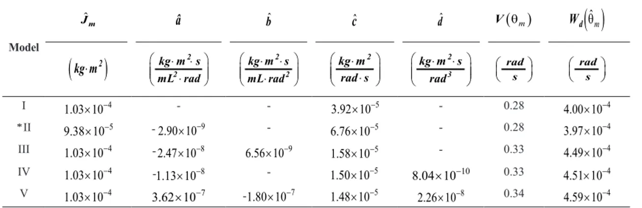
θˆe.

Although the Models I and II have presented the same

( )

m

V θ in Table 2, Model II was chosen for mechanical

dynamics because it exhibted the lowest

( )

ˆ

d m

W θ .

As seen in Table 3, the Model III was chosen as the initial model for hydraulic dynamics with minimum

( )

h

V θ , but the estimated static curves did not track the

reference curves, represented by the high value of the

( )

ˆ

d h

W θ . In sequence, the Model IV was analyzed, in which

the estimated curves provided a good representation of

the experimental data with lowest

( )

ˆ

d h

W θ .

Furthermore, the comparison between the measured and estimated signals for the electrical model, mechanical Model II and hydraulic Model IV, are shown in Figures 9a, 9b and 9c, respectively.

Thus, the static performance curves obtained experimentally and its rebuilding using the hydraulic Model IV can be observed in Figure 10.

Table 1. Estimated parameters for 0D model - electrical subsystem.

ˆ

a

R Lˆ_a kˆ_e V

( )

θ_e W _d

( )

θˆ_e

(Ω) ( mH )

V s rad ⋅    

  (A) (A)

1.87 38.82 2

1.24 10× − 4.06 10× −3 6.24 10× −5

Table 2. Estimated parameters for 0D model - mechanical subsystem.

Model ˆ

m

J â _bˆ _{cˆ d}ˆ V

( )

θ_m W _d

( )

θˆ_m

(

kg m ⋅ 2

)

 ⋅ ⋅     _⋅    2 2

kg m s mL rad  ⋅ ⋅     _⋅    2 2

kg m s mL rad  ⋅     _⋅    2 kg m rad s  ⋅ ⋅        2 3

kg m s rad       rad s       rad s I 4

1.03 10× − - - 3.92 10× −5 - 0.28 4.00 10× −4

*II 5

9.38 10 × − -2.90 10× −9 - 6.76 10× −5 - 0.28 3.97 10× −4

III 4

1.03 10× − - 8

2.47 10× − 6.56 10× −9 1.58 10× −5 - 0.33 4.49 10× −4

IV 4

1.03 10× − - 8

1.13 10× − - 1.50 10× −5 10

8.04 10× − 0.33 4.51 10× −4

V 4

1.03 10× − 3.62 10× −7 -1.80 10× −7 1.48 10× −5 8

2.26 10× − 0.34 4.59 10× −4

Table 3. Estimated parameters for 0D model - hydraulic subsystem.

Model

ˆ p

R Fˆp βˆ Lˆp Jˆp V

( )

θh W d

( )

θˆh

⋅      

mmHg s mL  ⋅        2 2 mmHg s mL  ⋅        2 2 mmHg s rad  ⋅        2 mmHg s mL  ⋅        2 mmHg s rad       mL s       mL s

I 7.88 - - 3

3.71 10× − - - 5.27 3

3.53 10× −

II 8.06 -0.04 _- 4

9.51 10× − - - 1.06 3

2.23 10× −

III 7.43 -0.04 - 4

9.89 10× − - 0.07 0.95 3

1.91 10× −

*_IV 2.51 0.01 - 3

1.14 10× − 0.68 - 1.04 4

1.92 10× −

V 2.47 0.01 _- 3

1.11 10× − 0.69 -5.16 10× −5 1.05 4

Discussion

With the experimental test setup and the characterization procedure, it was possible to find a suitable model for pRBP prototype. The pRBP dynamic model is composed of three coupled differential equations, the first one for the electrical subsystem, the second for the mechanical subsystem and the third one for the hydraulic subsystem. For the parameter estimation, the ERLS algorithm was adopted. The electrical parameters are given in Table 1, the mechanical parameters are given in Table 2 (line marked with a star), and the hydraulic parameters are given in Table 3 (line marked with a star).

Besides that, the pump characterization procedure provided a simple methodology for determining the

Figure 9. (a) Comparing i_a

( )

t and ˆia( )t ; (b) Comparing ω

( )

t and ωˆ

( )

t ; (c) Comparing q t

( )

and q tˆ

( )

.

Figure 10. The ∆ ×p q and ∆ ×p qˆ curves for the pRBP.

values of the continuous-time model parameters requiring

relatively few a priori information, specifically in

respect to the behavior of the mechanical and hydraulic subsystems. It is important to point out that the proposed characterization procedure is quite generic and can be applied when there are structural changes in the experimental setup, for example, the use a different type of motor or a pump with a different impeller type.

Also, it has been recognized, during the static tests as described in (Ganushchak et al., 2006), that if this pRBP operates in the area to the right of the operating zone

(in this work, ω > 4000 RPM) causes extreme turbulence

and cavitation. Even if this pRBP operates in the area

to the left of the zone (in this work, ω < 1000 RPM), its

operation is very inefficient, with excessive recirculation of fluid inside the pump and cavitation.

The application of the proposed methodology to a new pump where the motor is a BLDC type is underway. On the other hand, the connection of the pRBP prototype to an in vitro cardiovascular simulator is also underway.

Acknowledgements

The authors thank COPELE-PPgEE, CNPq, FAPESP Grant 201250283-6 and FINEP Grant 01.14.0177.00 for the financial support to the development of this project.

References

Capoccia M. Development and characterization of the arterial windkessel and its role during left ventricular assist device assistance. Artif Organs. 2015; 39(8):E138-53. http://dx.doi. org/10.1111/aor.12532. PMid:26147912.

Chen H. Extended recursive least squares algorithm for nonlinear stochastic systems. In: Proceedings of the American Control Conference; 2004 June 30-July 2; Boston, Massachusetts, USA. USA: IEEE Control Systems Society; 2004. p. 4758-63. http://dx.doi.org/10.23919/ACC.2004.1384065.

Choi S, Boston JR, Thomas D, Antaki JF. Modeling and identification of an axial flow blood pump. In: Proceedings of the 1997 American Control Conference (Cat. No.97CH36041); 1997 Jun 6-6; Albuquerque, New Mexico, USA. USA: IEEE Control Systems Society; 1997. p. 3714–5. http://dx.doi. org/10.1109/ACC.1997.609538.

Edwards Lifesciences Corporation. Truwave disposable pressure transducer [Internet]. Irvine: USA Edwards Lifesciences LLC; 2018. [cited 2018 June 16]. Available from: http://www.edwards. com/eu/products/pressuremonitoring/pages/truwave.aspx Ganushchak Y, van Marken Lichtenbelt W, van der Nagel T,

de Jong DS. Hydrodynamic performance and heat generation

by centrifugal pumps. Perfusion. 2006; 21(6):373-9. http:// dx.doi.org/10.1177/0267659106074003. PMid:17312862.

Germany em-tec GmbH. Experts in non-invasive flow measurement [Internet] [cited 2018 June 16]. Berlin: Germany em-tec GmbH; 2018. Available from: http://www.em-tec.com/ Jahanmir S, Hunsberger AZ, Heshmat H, Tomaszewski MJ, Walton JF, Weiss WJ, Lukic B, Pae WE, Zapanta CM, Khalapyan

TZ. Performance characterization of a rotary centrifugal left

ventricular assist device with magnetic suspension. Artif Organs. 2008; 32(5):366-75. http://dx.doi.org/10.1111/j.1525-1594.2008.00559.x. PMid:18471166.

Lim E, Cloherty SL, Reizes JA, Mason DG, Salamonsen RF,

Karantonis DM, et al. A dynamic lumped parameter model of the left ventricular assisted circulation. In: Proceedings

of the 29th Annual International Conference of the IEEE Engineering in Medicine and Biology Society; 2007 Aug 22-26; Cité Internationale, Lyon, France. USA: IEEE Engineering in Medicine and Biology Society; 2007. p. 3990-3. http://dx.doi. org/10.1109/IEMBS.2007.4353208. PMid: 18002874.

Ljung L. System identification: theory for the user. 2nd ed.

New Jersey: Prentice Hall; 1987.

Lubin T, Mezani S, Rezzoug A. Experimental and theoretical analysis of axial magnetic coupling under steady-state and

transient operation. IEEE Trans Ind Electron. 2014; 61(8):4356-65. http://dx.doi.org/10.1109/TIE.2013.2266087.

Moazami N, Fukamachi K, Kobayashi M, Smedira NG,

Hoercher KJ, Massiello A, Lee S, Horvath DJ, Starling

RC. Axial and centrifugal continuous-flow rotary pumps: A

translation from pump mechanics to clinical practice. J Heart Lung Transplant. 2013; 32(1):1-11. http://dx.doi.org/10.1016/j. healun.2012.10.001. PMid:23260699.

Moscato F, Danieli GA, Schima H. Dynamic modeling and

identification of an axial flow ventricular assist device. Int J Artif Organs. 2009; 32(6):336-43. http://dx.doi. org/10.1177/039139880903200604. PMid:19670185. Pennings KA, Martina JR, Rodermans BF, Lahpor JR, van de

Vosse FN, de Mol BA, Rutten MC. Pump flow estimation from pressure head and power uptake for the Heartassist5, Heartmate II, and Heartware VADs. ASAIO J. 2013; 59(4):420-6. http:// dx.doi.org/10.1097/MAT.0b013e3182937a3a. PMid:23820282.

Pérez CM. Bombas centrífugas como asistencia ventricular: estado actual. Cir Cardiov. 2009; 16(2):119-24. http://dx.doi. org/10.1016/S1134-0096(09)70156-1.

Pirbodaghi T, Weber A, Carrel T, Vandenberghe S. Effect

of pulsatility on the mathematical modeling of rotary blood

pumps. Artif Organs. 2011; 35(8):825-32. http://dx.doi. org/10.1111/j.1525-1594.2011.01276.x. PMid:21793862. Pirbodaghi T. Mathematical modeling of rotary blood pumps

in a pulsatile in vitro flow environment. Artif Organs. 2017; 41(8):710-6. http://dx.doi.org/10.1111/aor.12860. PMid:28097669. Santina M, Stubberud AR. Discrete-time equivalents of continuous-time systems. In: Levine WS, editor. The control

handbook: control system fundamentals. Boca Raton: CRC Press; 2010. p. 12.1-12.34.

Shi Y, Lawford P, Hose R. Review of zero-D and 1-D models of blood flow in the cardiovascular system. Biomed Eng Online. 2011; 10(33):1-38. http://dx.doi.org/10.1186/1475-925X-10-33. PMid:21521508.

Stanfield JR, Selzman CH, Pardyjak ER, Bamberg S. Flow characteristics of continuous-flow left ventricular assist devices in a novel open-loop system. ASAIO J. 2012; 58(6):590-6. http:// dx.doi.org/10.1097/MAT.0b013e31826dcbd9. PMid:22990285.

Stanfield JR, Selzman CH. In vitro pulsatility analysis of axial-flow and centrifugal-flow left ventricular assist devices. J Biomech Eng. 2013; 135(3):0345051-6. http://dx.doi. org/10.1115/1.4023525. PMid:24231821.

Zhang XT, AlOmari AH, Savkin AV, Ayre PJ, Lim E, Salamonsen RF, et al. In vivo validation of pulsatile flow and differential

pressure estimation models in a left ventricular assist device.

In: Proceedings of the Annual International Conference of the IEEE Engineering in Medicine and Biology; 2010 31 Aug-4

Sept; Buenos Aires, Argentina. USA: IEEE Engineering in