Anthromes displaying evidence
of weekly cycles in active fire data
cover 70% of the global land surface
J. M. c. pereira
1, M. A. Amaral Turkman
2, K. f. Turkman
2& D. oom
1Across the globe, human activities have been gaining importance relatively to climate and ecology as the main controls on fire regimes and consequently human activity became an important driver of the frequency, extent and intensity of vegetation burning worldwide. Our objective in the present study is to look for weekly cycles in vegetation fire activity at global scale as evidence of human agency, relying on the original MODIS active fire detections at 1 km spatial resolution (MCD14ML) and using novel statistical methodologies to detect significant periodicities in time series data. We tested the hypotheses that global fire activity displays weekly cycles and that the weekday with the fewest fires is Sunday. We also assessed the effect of land use and land cover on weekly fire cycle significance by testing those hypotheses separately for the Villages, Settlements, Croplands, Rangelands, Seminatural, and Wildlands anthromes. Based on a preliminary data analysis of the daily global active fire counts periodogram, we developed an harmonic regression model for the mean function of daily fire activity and assumed a linear model for the de-seasonalized time series. For inference purposes, we used a Bayesian methodology and constructed a simultaneous 95% credible band for the mean function. The hypothesis of a Sunday weekly minimum was directly investigated by computing the probabilities that the mean functions of every weekday (Monday to Saturday) are inside the credible band corresponding to mean Sunday fire activity. Since these probabilities are small, there is statistical evidence of significantly fewer fires on Sunday than on the other days of the week. Cropland, rangeland, and seminatural anthromes, which cover 70% of the global land area and account for 94% of the active fires analysed, display weekly cycles in fire activity. Due to lower land management intensity and less strict control over fire size and duration, weekly cycles in Rangelands and Seminatural anthromes, which jointly account for 53.46% of all fires, although statistically significant are weaker than those detected in croplands.
Across the globe, human activities have been gaining importance relatively to climate and ecology as the main controls on fire regimes, and during the last few decades anthropogenic vegetation burning expanded its impact on land cover, ecosystem dynamics, and atmospheric greenhouse gas emissions from regional to global scales1–4. Human activity became a significant driver of the frequency, extent and intensity of vegetation burning world-wide, and the timing of ignitions is strongly dependent on human agency5,6. Fire temporal patterns are a function of climate dynamics and human activity, with periodic cycles found at annual scale in seasonally dry areas, and at the daily scale in response to underlying cycles in meteorological variables and land management activities6,7. Fire regimes have been modified to manage croplands, rangelands, forests, and wildlife, to protect infrastructure and settled areas8, as a form of political protest9, and to wage war10. Predictability of spatial and temporal fire patterns increases with the length of human presence and the degree of human dominance over the landscape11. Vegetation burning has been analyzed at time scales ranging from daily7 to annual12, centennial13, and millen-nial14,15. It is a large source of greenhouse gases and aerosols and constitutes a major factor controlling variability of atmospheric composition at the inter-annual scale16.
Approaches to isolate the impact of anthropogenic aerosol on clouds from natural cloud variability were reviewed by17 and included the detection of weekly cycles, because seven-day periodicities are highly unlikely due to natural forcing, and thus provide strong evidence of anthropogenic perturbations. Weekly cycles over 1Centro de Estudos Florestais, Instituto Superior de Agronomia, Universidade de Lisboa, Lisboa, Portugal. 2Centro de Estatística e Aplicações, Faculdade de Ciências da Universidade de Lisbon, Lisboa, Portugal. Correspondence and requests for materials should be addressed to M.A.A.T. (email: [email protected])
Received: 3 January 2019 Accepted: 17 July 2019 Published: xx xx xxxx
broad geographical areas cannot be explained by the reduction in industrial and transportation emissions in urban areas alone. The possible anthropogenic influence on these cycles remains unclear, but different processes are required to explain their occurrence. The most plausible hypothesis to interpret large-scale weekly cycles is through direct and indirect effects of anthropogenic aerosols, whose emissions also tend to show weekly perio-dicity at large-scale18. A weekly cycle of aerosol optical depth (AOD), observed in the United States and in Central Europe, was stronger in urban sites than in rural sites. A different weekly cycle detected in the Middle East and India had lower AODs on Thursday and Friday, the weekend for Middle Eastern cultures19. Close synchrony between weekly peaks in anthropogenic aerosols and tornado activity over the eastern US during the summer was detected by20. They found a statistically significant weekly cycle in storm activity during summer for the period 1995 to 2009, unlikely to be due to natural variability. A connection with fire activity was provided by21 in their analysis of an historical tornado outbreak in the southeastern U.S., where they proposed that smoke from biomass burning in Central America might have increased tornado severity due to boundary-layer stabilization by soot and an increase in the optical thickness of lower tropospheric clouds. The assumption that vegetation burning is a natural aerosol source, and thus does not display weekly cycles, was adopted in the analyses of20 and21, as well as in the atmospheric chemistry modelling studies of22 and17. However,23 found significantly weekly cycles in sub-Saharan Africa cropland burning, with Sunday minima in predominantly Christian regions and Friday minima in mainly Muslim regions. They did not find significant weekly cycles in fire activity in densely settled areas, where vegetation burning is very limited, nor in rangelands, forests and wildlands, where fire management intensity is weaker than in croplands.
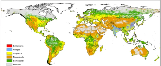
These continental-scale findings, combined with the recognition of the strongly anthropogenic nature of global vegetation burning24 motivated the hypothesis of weekly cycles in global fire activity, as observed with remotely sensed active fire data. The hypothesis of a Sunday weekly minimum in fire activity has two justifica-tions: (i) international labour legislation stipulates a weekly day of rest, which in most countries is Sunday, and (ii) of the two major global religions (Christianity and Islam) that prescribe a weekly day of rest, Christianity prevails in more high fire incidence areas. We also assessed the effect of land use and land cover on weekly fire cycle significance by testing the aforementioned hypotheses separately for the Villages, Settlements, Croplands, Rangelands, Seminatural, and Wildlands anthropogenic biomes (anthromes)25, which map global patterns of sustained direct human interaction with ecosystems. Anthrome-specific analysis provides valuable information to elucidate the land management activities, regions, and times of the year contributing to the occurrence of weekly cycles in global vegetation burning.
Previous research by26 and27 also detected Sunday minima in global fire activity, using spatially aggregated fire counts data from the NASA Earth Observations website (http://neo.sci.gsfc.nasa.gov/view.php?datasetId=− MOD14A1_M_FIRE). However, inconsistencies between the active fire numbers reportedly used by26 and by27, and their discrepancies relatively to other published sources justify revisiting the topic of weekly cycles in global active fire data. Their data differ from those published by various other sources in the number of MODIS active fires reportedly used, in the time series of annual active fire numbers, and in the weekly distribution of active fires. In comparison with all other published sources that have partially overlapping study periods and mention the numbers of active fires used,26 claim having worked with many more fires, while27, who used a time series three years longer than that of26, surprisingly report substantially fewer fires. Table 1 in Supplementary Information shows the numbers involved in these comparisons. The discrepancies between26 and27 relatively to other authors are largest for the first two years of their time series, 2001 and 2002, which they claim to have the most active fires. This is an obvious impossibility, since during all of 2001 and the first half of 2002, only the TERRA instrument, which has a morning overpass at 10:30AM/PM, was in orbit. AQUA was launched in mid-2002 with a 2:30AM/ PM overpass and that more than doubled the amount of active fires detected because the AQUA daytime overpass observes the most active period of the diurnal cycle of vegetation burning. Figure 5 of28 displays the relative con-tribution of AQUA to the total MODIS active fire detections and clearly shows that AQUA detections account for more than half of all active fires. Therefore, the number of active fires in the MODIS data product (MCD14ML) for the years 2001 and 2002 is less than half of that in each subsequent year, as shown in figure 2a of29. Table 1 in Supplementary Information provides specific comparisons for these two years, taking into account differences in the MODIS sensors and in the active fire data collections used by the various authors. There are also differences between the weekly distributions of MODIS active fire counts shown in figure 2a of26 and in figure 4 of27, and the distribution portrayed in Fig. 1 below. In the original MDC14ML data that we used the relative difference between the numbers of active fires on Sunday and Monday is larger, i.e., Sunday is a more prominent weekly minimum and Tuesday is a more prominent weekly maximum, and thus the magnitude of the weekly cycle in the number of active fires is larger. In addition, there is a change in rank order of the number of active fires by weekday with Friday, rather than Monday, having the second fewest fires. These differences are likely to affect the results of a weekly cycle analysis.
The paper by26 also has some methodological issues. In our opinion, the statistical tests they used to detect and characterize weekly fire cycles, may not be adequate to answer two fundamental questions: (i) if there is evidence in the data that there are 7 day cycles (ii) If there is such evidence in the data, fire activity in each day of the week have different statistical properties, in particular, if average Sunday fire counts are less that the average counts in other days of the week. Daily counts of fire activity constitute a time series and by nature, they show strong and complex temporal dependence structures. Without accounting for such temporal dependence structures it is not possible to come up with correct conclusions on (i) and (ii). The authors26 base their results on statistical methods, which we believe, do not take into account proper time series analysis. Although their Monte Carlo tests may show the extent to which a weekly cycle is present under random conditions, and thus the probability that the weekly pattern of fire counts observed in the data occurs by chance, they do not test the shape, nor even the exist-ence of such a cycle. Their subsequent Kolmogorov-Smirnov test only shows, for the global scale analysis, that the two days of the week displaying the largest and smallest number of fires (Tuesday and Sunday respectively) have
distinct statistical distributions. This, by itself, does not provide evidence that there is a minimum on Sunday fire activity, neither shows that the activity on Sunday differs from the other days of the week.
Our goal in the present study is to reanalyse the topic of weekly cycles in vegetation fire activity at global scale, relying on the original MODIS active fire detections at 1 km spatial resolution (MCD14ML) with appropriate statistical methodologies to detect significant periodicities in time series data. Using Bayesian methodology, a simultaneous 95% credible band for the mean function was constructed. Sunday minimum is hence directly investigated by computing the probabilities that the mean functions of every week day (Monday to Saturday) are inside the credible band corresponding to mean Sunday fire activity.
Data
Daily fire activity data were obtained from the NASA MODIS MCD14ML Collection 5 active fire product30 at 1 km spatial resolution, after screening for false alarms and non-vegetation fires according to the procedures detailed in29. We analysed the period from July 8, 2002 to July 29, 2012 (TERRA and AQUA sensors), for a total of 525 full weeks and 43,416,629 fire counts. Figure 1 shows the mean + 1 sd. of total fire counts per weekday. Land use/land cover data used are from the Anthropogenic Biomes of the World (anthromes) dataset, at 5′ (ca. 9 km) spatial resolution, dated from the year 2000. Anthrome data combine information on population density, land cover and land use to derive a map of global patterns of sustained direct human interaction with ecosystems25. Since a large majority of global vegetation burning is anthropogenic24, they were considered particularly appro-priate for our analysis. The relative stability of spatial patterns depicted by the anthromes dataset further justifies its use in conjunction with global fire activity data for the period 2002 to 2012.
Each active fire was labeled with the anthrome class present at its geographical coordinates to create the data-sets for the anthrome-specific fire weekly cycle analyses (see Table 1). Maps aggregated at 0.5° spatial resolution of the weekday with the fewest fires and of Global Anthromes (v2.0) using the modal class rule are shown in Figs 2 and 3 respectively.
Methods and Models
Preliminary data analysis and sampling model identification.
To search for weekly cycles invegeta-tion burning, we analysed a 525-week time series of global daily MODIS active fire counts.
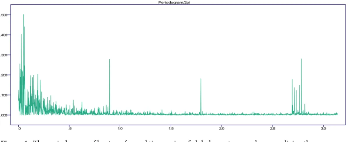
The sample auto correlation (acf) and the partial auto correlation function (pcf) together with the periodo-gram of the log-transformed daily global fire count data were used to search for periodical variations in the data. The periodogram was calculated to identify frequencies at which jumps occur and their significance was tested with Fisher’s test and Whittle’s test31,32.
Mon Tue Wed Thu Fri Sat Sun
week day mean 11883 12310 12102 12027 11809 11955 10613 02 00 04 000 600 08 00 01 0000 1200 01 4000 1600 01 8000
Figure 1. Mean + 1.s.d. active fire counts per weekday for the entire study period. Tuesday, Wednesday and
Thursday are the weekdays with the highest fire count averages, exceeding 12,000; Monday, Friday and Saturday all exceed 11,000 counts, and Sunday is the only day with a fire count average below 11,000.
Anthromes Settlements Villages Croplands Rangelands Seminatural Wildlands
fires 139420 1545653 17043106 9111319 13555751 1006472
% 0.33 3.65 40.19 21.49 31.97 2.37
The periodogram showed statistically significant jumps at the fundamental frequency wj = 2πj/365
corre-sponding to 1 cycle in 365 days and its first 3 harmonics, correcorre-sponding respectively to 1 cycle in 6 months, 4 months, and 3 months. De-seasonalizing the data by fitting an harmonic regression at these frequencies unmasked further jumps in the periodogram at frequencies corresponding respectively to 1 cycle in 7 days and 1 cycle in 3 and half days. Further application of Whittle’s test showed that these two jumps are also statistically significant. Figure 4, shows the periodogram of the deseasonalized series where these jumps are quite evident. Jumps on the right hand side of the periodogram correspond to high frequency noise.
Results of the spectral analysis clearly suggest that the log transformed global daily fire count time series Yt is
non-stationary, and that its mean function Mt should include a harmonic sum with k = 6 harmonics
correspond-ing to the angular frequencies of 1 cycle per year, per 6, 4, and 3 months, and per 7, and 3.5 days. We then suggest the model Yt = Mt + Xt, with Xt a stationary error term. Detailed study of the deseasonalized series by using the
software ITSM31 suggested that the stationary component of the time series X
t is well represented by a zero mean
stationary and invertible Gaussian Autoregressive model of order 7 (AR(7)).
The annual and multi-month cycles in fire activity result from global climate seasonality patterns, including the lagged dry seasons of the Northern and Southern hemispheres, as well as the occurrence of fire seasons in the tropical savannas of the Northern hemisphere during the boreal winter6,33. We hypothesize that the weekly cycle is an anthropogenic fingerprint, due to weekly days of rest determined by religious norms and labor regulations. Figure 1 shows that there are four consecutive weekdays with a mean number of fires under 12,000 (Friday to Monday), followed by three days with over 12,000 fire counts (Tuesday to Thursday). Since Friday is a religious holiday for Muslims in the extensively burned sub-Saharan region of Northern hemisphere Africa, Saturday is
Figure 2. Weekday with the fewest fire counts, 2002–2012.
a civil day of rest, and Sunday is simultaneously a civil and religious holiday in most of the western world, the reduced fire activity during these days is understandable. The inclusion of Monday in this group of days may be a spillover effect from the previous days. The period Tuesday to Thursday is not affected by imposed weekly days of rest and thus the use of fire as a land management tool increases.
Bayesian model and inference.
Following the preliminary data analysis we assumed the following modelfor the time series of log-transformed daily global fire count data
= +
Yt Mt X ,t (1)
where the mean function Mt is
∑
ω ω = + + + = M a a t [ cosc t d sin ],t (2) t i i i i i 0 1 1 6with angular frequencies ωi, i = 1,2, .. 6 corresponding to the significant jumps identified in the periodogram and
∑
φ = + = − Xt X Z i 1 i t i t 7is a stationary, zero mean process compatible with a stationary and invertible Gaussian AR(7) process, where, Zt
is a zero mean, uncorrelated (white noise) process.
For the vector of parameters of the fixed effects (a1, ci, di, i = 1, ..., 6) we considered independent normal priors
with zero mean and precision 0.001 and a flat prior for a0. For the parameters of the AR(7) process, (φ1, ..., φ7) we used, after a transformation of the parameter space, penalised complexity priors for the partial autocorrelation functions, as suggested by34.
We fitted this model within the R-INLA environment35, in which the mean function M
t and the stationary
process Xt appear respectively as the fixed and random effects in the linear model specification.
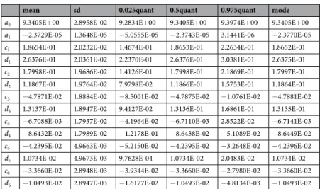
From the analysis of the model, we observe from Table 2 that all the harmonic coefficients are significant, but there is no evidence of a linear trend.
Comparing the mean functions.
Once we establish that fire activity indeed displays weekly cycles, it isinteresting to see in which day of the week the minimum fire activity is observed, in particular, one may want to test the hypothesis that the fire activity is minimum on Sundays. One way of answering this question is to com-pare the mean functions Mti in (2) with ti = i, i + 7, i + 14, ... and i = 1, ..., 7, where i = 1 refers to Monday and i = 7 refers to Sunday. That is compare the mean functions corresponding to the fire activity series of different days of the week.
Our strategy to test the hypothesis that the fire activity is minimum on Sundays will be based on calculating the 95% simultaneous credible interval (credible band) corresponding to Sunday mean function Mt7 and (i) check how likely is the mean function of other days of the week falling within this credible band. Additionally we com-pute the probabilities that the mean functions of other days of the week are above the estimated mean function of Sunday (ii). Significant lower probabilities of (i) and significant higher probabilities of (ii) give evidence that indeed fire activity is minimum on Sundays. We explain below the computational details.
The marginal posterior distribution for the mean function Mt, t = 1, ..., 3765 is approximately multivariate
normal with posterior mean ˆM tt, =1,…, 3765 and posterior covariance matrix S35, which can be obtained from R-INLA using inla.make.lincomb function. Pointwise 100(1 − γ)% HPD (highest posterior density) intervals for each component of the vector Mt can also de obtained using the function inla.hpdmarginal. Figure 4. The periodogram of log transformed time series of global counts upon deseasonalizing the
However, rather than obtaining pointwise credible intervals, one should seek for a simultaneous credible band for Mt of size 100(1 − α)%. For that we follow the suggestion given by36.
For the random vector {Mt, t = 1, ..., n} = (M1, ..., Mn), a 100(1 − α)% simultaneous credible band can be
defined as a hyper-rectangular region
∩
=
{
=(
∈ γ)
}
R { }:Mt in M I
i i
1 ,
where {Ii,γ}, i = 1, ..., n denotes a set of individual 100(1 − γ)% HPD credible intervals for each component of the
vector Mt, with γ chosen so that P({Mt} ∈ R) = 1 − α.
Since the posterior distribution for the vector Mt is approximately multivariate normal with known mean
vector and known covariance matrix, by trial and error, one can obtain a simultaneous 100(1 − α)% HPD credible band for the vector {Mt, t = 1, ..., n}, by computing, for every individual component of the vector, a 100(1 − γ)%
HPD credible interval, varying γ till the overall probability is 1 − α. α
= … ∈ = − .
P M t({ ,t 1, , }n R) 1
Actually this can also be obtained using the function excursions.simconf available in the R package excursions37.
Considering the fact that the linear trend was not significant and considering the cyclic nature of Mt, above
calculations were reported for the first 52 weeks, rather than for the full period.
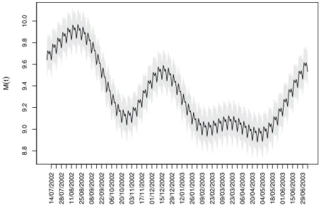
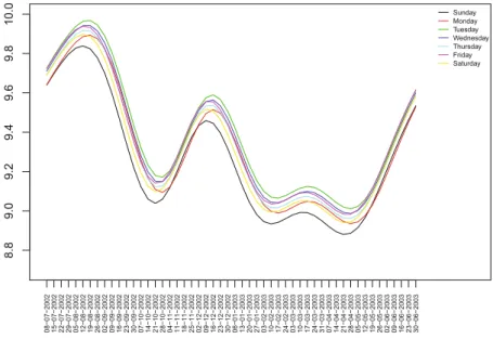
In Figure 5 we display the series of the log counts with the estimated mean function (posterior mean) ˆMt, and in Fig. 6 the estimated mean function for the first year, ie, ˆM tt, =1,…, 364 together with the 95% simultaneous credible band.
mean sd 0.025quant 0.5quant 0.975quant mode
a0 9.3405E+00 2.8958E-02 9.2834E+00 9.3405E+00 9.3974E+00 9.3405E+00
a1 −2.3729E-05 1.3648E-05 −5.0555E-05 −2.3743E-05 3.1441E-06 −2.3770E-05
c1 1.8654E-01 2.0232E-02 1.4674E-01 1.8653E-01 2.2634E-01 1.8652E-01
d1 2.6376E-01 2.0361E-02 2.2370E-01 2.6376E-01 3.0381E-01 2.6375E-01
c2 1.7998E-01 1.9686E-02 1.4126E-01 1.7998E-01 2.1869E-01 1.7997E-01
d2 1.1867E-01 1.9764E-02 7.9798E-02 1.1866E-01 1.5753E-01 1.1864E-01
c3 −4.7871E-02 1.8884E-02 −8.5001E-02 −4.7875E-02 −1.0761E-02 −4.7881E-02
d3 1.3137E-01 1.8947E-02 9.4127E-02 1.3136E-01 1.6861E-01 1.3135E-01
c4 −6.7088E-03 1.7937E-02 −4.1964E-02 −6.7110E-03 2.8522E-02 −6.7141E-03
d4 −8.6432E-02 1.7989E-02 −1.2178E-01 −8.6438E-02 −5.1089E-02 −8.6449E-02
c5 −4.2395E-02 4.9663E-03 −5.2150E-02 −4.2395E-02 −3.2648E-02 −4.2396E-02
d5 1.0734E-02 4.9673E-03 9.7628E-04 1.0734E-02 2.0483E-02 1.0734E-02
c6 −3.3660E-02 2.8948E-03 −3.9344E-02 −3.3660E-02 −2.7980E-02 −3.3660E-02
d6 −1.0493E-02 2.8947E-03 −1.6177E-02 −1.0493E-02 −4.8134E-03 −1.0493E-02
Table 2. Summary Statistics for the posterior distribution of the fixed effects.
log(counts) 08/07/200 2 08/07/200 3 08/07/200 4 08/07/200 5 08/07/200 6 08/07/200 7 08/07/200 8 08/07/200 9 08/07/201 0 08/07/201 1 08/07/201 2 7.2 7.6 8.0 8. 48 .8 9.2 9.6 10.0 10.4
Since the posterior distribution of the mean function Mt is multivariate normal, Mt can be partitioned into
= ...
M iti, 1, , 7 (with 1 for Monday, 7 for Sunday), as explained before, to represent the mean functions for the different days of the week. Properties of the multivariate normal distribution imply that the posterior distribu-tions of Mti, ti = i, i + 7, ... and i = 1, ..., 7 are also approximately multivariate normal with means given by the ˆMti, ti = i, i + 7, ... and i = 1, ..., 7 and corresponding covariance matrices, which are sub-matrices of the overall
covar-iance matrix. Also if we represent the 100(1 − α)% HPD credible bands for Mt by the two series LBt and UPt, they
can similarly be partitioned into LBti and UPti, for i = 1, ..., 7.
We propose as a methodology to test the hypothesis that there is, on average, smaller fire activity on Sundays, by computing the probabilities, for i = 1, ..., 6
≤ ≤
(
)
P LBt7 Mti UB ,t7
that is, the probabilities that the mean function for every day of the week is inside the credible bands correspond-ing to Sunday, ie, inside LBt7 and UPt7. These probabilities can be easily obtained using the function gaussint() from the R package excursions37.
In Table 3 we show these probabilities, with the associated error in brackets, computed using the first year. For the other years the results are very similar.
We also compute the posterior probabilities that the mean function for every other week day M iti, =1, , 7... is above the estimated mean function for Sunday (the mean of the posterior distribution of the mean vector Mt7). These probabilities are given in Table 4.
From Table 3 we observe that, besides Saturday, the mean functions of all the other days of the week have lower probabilities of being inside the credible band for Sunday. Also from Table 4 we observe that except for Monday, all other days of the week have relatively high probabilities of being above the estimated mean function of Sunday. Hence there is some evidence that, in general, minimum fire activity is indeed on Sundays.
Figure 7 is an unfolded reproduction of Fig. 6, that is, the estimated mean function ˆMt is partitioned into ˆMti, ti = i, i + 7, i + 14, ..., and i = 1, ..., 7 to represent the estimated mean function for the different days of the week.
M ( t ) 14/07/2002 28/07/2002 11/08/2002 25/08/2002 08/09/2002 22/09/2002 06/10/2002 20/10/2002 03/11/2002 17/11/2002 01/12/2002 15/12/2002 29/12/2002 12/01/2003 26/01/2003 09/02/2003 23/02/2003 09/03/2003 23/03/2003 06/04/2003 20/04/2003 04/05/2003 18/05/2003 01/06/2003 15/06/2003 29/06/2003 8. 89 .0 9. 29 .4 9.6 9.8 10. 0
Figure 6. Estimated posterior mean function ˆM tt, =1,…, 364 together with the 95% simultaneous credible bands (in grey).
Monday Tuesday Wednesday Thursday Friday Saturday Sunday
0.1965
(0.0036) 0.0066(0.0006) 0.0712(0.0022) 0.3140(0.0041) 0.2041(0.0033) 0.7019(0.0039) 0.9696(0.0013)
Table 3. Probabilities that mean functions for the logarithm of the fire counts for each day of the week are
inside the 95% simultaneous credible band for Sunday.
Monday Tuesday Wednesday Thursday Friday Saturday Sunday
P 0.0556(0.0012) 0.7644(0.0033) 0.6303(0.0037) 0.4531(0.0037) 0.7412(0.0034) 0.3511(0.0036) 0.0172(0.0007)
Table 4. Probabilities =P P M( ti> ˆMt7) that mean functions for the logarithm of the fire counts for each day of the week are above the estimated mean function for Sunday.
For ease of reading, only the first year is plotted. Other years have the same behaviour, due to the cyclic nature of the mean function, since the linear trend is not statistically significant.
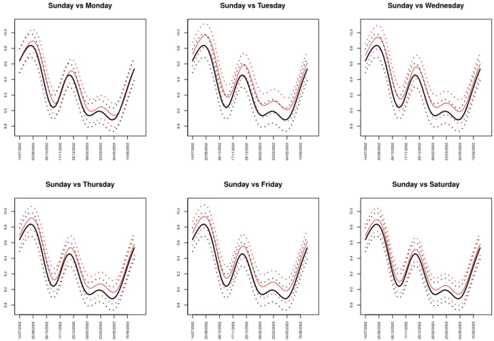
It is clear from that plot that the estimated mean function corresponding to Sunday fire counts is smaller than the other estimated mean functions almost uniformly for every week. Looking in more detail we remark that the estimated mean function for Sunday shows always lower values, except for the period ranging from the second week of November to the first week of December and from the third week of May until the end of June, when it is always very close to the estimated mean function for Monday. The second minimum is basically on Saturday or Monday. This may indicate the existence of a weekend effect on daily fire counts. To understand how much smaller the estimated mean function for Sunday is from the other days of the week, we display in Fig. 8 the estimated mean function for Sunday together with the corresponding 95% simultaneous credible band and the estimated mean functions for each of the other days of the week. We observe that the estimated mean function for Saturday is always inside the credible band for Sunday and only during two periods of the year, namely, third week of August to third week of October and second week of December to the second week of April, the estimated mean functions for some of other days of the week are above the upper bound of the credible band for Sunday. (see detailed study in the technical report)38 (http://ceaul.org/wp-content/uploads/2018/10/NotaseCom_3_2016.
pdf). This is an indication that there is evidence of a weekly cycle with minimum on Sunday, only during these periods of the year.
Further, the comparison of fire activity in each day of the week involves comparison and ordering of time series, We note that existence of ordering for mean functions does not necessarily imply stochastic ordering for the respective time series. However the following result in39 gives an indication when ordering in mean functions imply respective stochastic ordering: If Xt and Yt are two independent Gaussian processes with the same
covar-iance structure and if E(Xt) ≤ E(Yt) uniformly for every t, then Xt is stochastically dominated by Yt. The precise
definition of stochastic ordering can be found in39. There is strong evidence in the data that deseasonalized log fire activity for each day of the week follow a AR(1) process and although they are certainly not independent, this might suggest that the results on comparison on the means may extend to respective stochastic ordering. However, further detailed work is needed to reach such complete conclusion.
Anthrome-level Analysis
The methodology shown in section 3.3 was applied to time series of the logarithm of the number of active fire counts described with each of the six anthromes shown in Fig. 3. Following their global analysis,26, searched for weekly cycles in regions of the globe displaying abundant fire activity. This approach designated40 post-hoc domain selection, and warn that it risks biasing the analysis, since it might be expected that regions experiencing many fires might exhibit large weekly cycles. In order to avoid the potential for this type of bias, we regionalised our analysis independently of any observed fire activity spatial patterns, based on the hypothesis that the likeli-hood of active fire weekly cycles vary by anthrome. Only for Croplands did Whitle’s test show strong evidence of significant jumps in the periodogram at frequency corresponding to weekly cycles, although some evidence is also observed for Rangelands and Seminatural anthromes. Table 5 and Fig. 9 show, for each anthrome, the proba-bilities that the mean function for every day of the week is inside the Sunday 95% credible band.
Complementary to these probabilities, we also calculated the probability that a mean function of a day of the week is above the estimated Sunday mean function. These probabilities are given in Table 6 (see also Fig. 10).
Comparing the probabilities between Sunday and other weekdays displayed on Tables 5 and 6 we can say that there is a strong evidence that for Croplands, the mean function for Sunday is statistically smaller than the mean function for every other day of the week. This evidence is not so strong for Rangelands and Seminatural since the probability that Saturday mean function is inside the 95% credible band for Sunday is relatively high.
For other anthromes there is no statistical evidence of a difference between the mean functions corresponding to the different days of the week. Globally, albeit with varied strengths of evidence, three anthromes (croplands, rangelands, and seminatural areas), corresponding to 70% of the land surface and to 94% of the active fire data analysed display weekly cycles in fire activity.
To understand how much smaller the estimated mean function for Sunday in Croplands is from the other days of the week, we display in Fig. 11 the estimated mean function for Sunday together with the 95% simultaneous credible band and the estimated mean functions for each of the other days of the week.
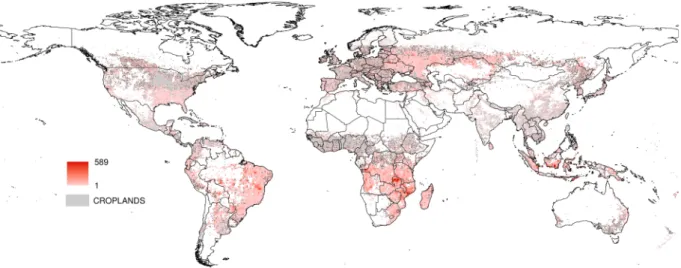
For each anthrome, we identified the longest uninterrupted period during which the estimated mean func-tion for the largest number of weekdays is above the 95% upper credible band for Sunday, representing the time of the year when the weekly cycle of fire activity is strongest. In the Cropland anthrome this period lasts from early September to early October, when vegetation burning takes place mostly in Southern hemisphere Africa, Brazil, Southeastern USA, Southwestern Russia and the Ukraine (see Fig. 12). The Seminatural anthrome weekly cycle is clearest at a similar time of the year (mid-September to early October) and has a partially overlapping
Figure 8. Estimated mean function of the logarithm of the fire counts for Sunday(in black) and corresponding
95% simultaneous credible band (black dots), with the estimated mean functions ˆMti of the logarithm of the fire counts for each other day of the week(in red) and corresponding simultaneous credible band(red dots).
Anthrome Monday Tuesday Wednesday Thursday Friday Saturday Sunday
Croplands 0.0122(0.0007) 0.0000(0.0000) 0.0002(0.0000) 0.0227(0.0012) 0.0013(0.0002) 0.3770(0.0040) 0.9750(0.0012) Rangeland 0.0455(0.0017) 0.0005(0.0002) 0.0145(0.0009) 0.1779(0.0032) 0.2051(0.0033) 0.7628(0.0037) 0.9724(0.0013) Seminatural 0.2684(0.0041) 0.0309(0.0014) 0.1153(0.0027) 0.2946(0.0040) 0.1890(0.0033) 0.6995(0.0039) 0.9673(0.0014) Wildland 0.7001(0.0043) 0.7898(0.0037) 0.8584(0.0032) 0.9026(0.0027) 0.9293(0.0023) 0.9487(0.0020) 0.9554(0.0020) Settlements 0.9011(0.0027) 0.8047(0.0035) 0.9164(0.0024) 0.9566(0.0018) 0.9729(0.0014) 0.9653(0.0015) 0.9770(0.0012) Villages 0.7517(0.0039) 0.5565(0.0045) 0.7974(0.0036) 0.9440(0.0020) 0.9384(0.0021) 0.9526(0.0019) 0.9742(0.0013)
Table 5. Anthrome-specific probabilities that mean functions for the logarithm of the fire counts for each day
geographical distribution (Southern hemisphere Africa and South America, Fig. 13). During this period, fire activity in Croplands during this strongly cyclic period displays a clear Sunday minimum and is concentrated in regions that are predominantly Christian and/or where labor regulations concerning a weekly period of rest
Figure 9. Anthrome-specific probabilities that mean functions for the logarithm of the fire counts for each day
of the week are within the 95% simultaneous credible band for Sunday: complementary to Table 5. Values in parenthesis represent the % of total active fires in the respective anthrome.
Anthrome Monday Tuesday Wednesday Thursday Friday Saturday Sunday
Croplands 0.0367(0.0012) 0.9273(0.0022) 0.8004(0.0032) 0.6606(0.0038) 0.9492(0.0017) 0.5014(0.0039) 0.0010(0.0001) Rangeland 0.0069(0.0003) 0.5622(0.0038) 0.4803(0.0037) 0.2961(0.0033) 0.5133(0.0038) 0.1209(0.0022) 0.0014(0.0002) Seminatural 0.0034(0.0003) 0.3630(0.0038) 0.3361(0.0037) 0.2981(0.0035) 0.5919(0.0040) 0.1801(0.0029) 0.0013(0.0002) Wildland 0.0001(0.0000) 0.0002(0.0000) 0.0002(0.0001) 0.0005(0.0001) 0.0010(0.0001) 0.0008(0.0002) 0.0012(0.0001) Settlements 0.0142(0.0008) 0.1173(0.0025) 0.0560(0.0017) 0.0041(0.0004) 0.0146(0.0007) 0.0522(0.0015) 0.0199(0.0008) Villages 0.0150(0.0006) 0.1597(0.0027) 0.0821(0.0019) 0.0172(0.0007) 0.0588(0.0015) 0.0664(0.0017) 0.0167(0.0007)
Table 6. Probabilities that the mean function for every day of the week is above the estimated mean function
for Sunday (error in brackets).
Figure 10. Probabilities that the mean function for every day of the week is above the estimated mean function
for Sunday: complementary to Table 6. Values in parenthesis represent the % of total active fires in the respective anthrome.
are enforced23,26. Evidence of a weekly cycle is weaker in the Seminatural anthrome and not so much as a Sunday minimum, but more as a weekend effect (Table 5). In Rangelands, the time of the year when the weekly cycle in vegetation burning is most evident goes from late December to early February. Fire activity is concentrated in the tropical savannas of the Northern hemisphere, mainly in Muslim sub-Saharan Africa (see Fig. 14). Unlike at other times of the year, fire counts on Thursday and Friday, the religious and civil days of rest in the region, are inside the credible band for Sunday fire counts, suggesting the influence of religious practices on the weekly fire cycle23.
Discussion and Conclusions
The present study revisited the topic of global weekly fire cycles, previously addressed by26 and27; We used original MCD14ML data, without any form of gridding or normalization of fire counts that appear to have caused the problems described in the Erratum of26. These problems were not fully corrected, as shown in the Supplementary Information Table 1, and cast doubt upon the reliability of their results. Our geographical stratification of the analysis was defined a priori, avoiding potential biases introduced by post-hoc spatial domain selection and relies on an explicit hypothesis that the likelihood and features of active fire weekly cycles are anthrome-specific. The anthrome-based spatial stratification provides insights into the influence of land use intensity on the occurrence of fire weekly cycles.
Employing statistical methodologies more appropriate for the detection of weekly cycles in time series of active fire counts, and for determining the weekday with the fewest fires, we reliably detected a weekly global fire activity cycle with a Sunday minimum, and Table 3 shows that for Saturday there is a reasonable probability that the corresponding mean function is inside the credible band for Sunday. Also, Figs 7 and 8 show that the esti-mated mean function for Sunday is almost everywhere below the estiesti-mated mean function for the weekdays and almost always very close or even below the lower confidence bounds of the week days. However, contrary to the other days of the week, the estimated mean function for Saturday is always inside the credible bands for Sunday. This finding, associated with the reasonable high probability 0.7019 displayed in Table 3, indicates that rather than a Sunday minimum, there actually is a weekend minimum in global active fire counts.
Our research expanded previous continental-scale work on weekly cycles of fire activity when the data are disaggregated by anthrome23, by identifying Croplands (40.19% of all fires) as the anthrome with the strongest fire weekly cycles, which reaffirms the importance of land management intensity as a driver of the cycles. Table 6 shows strong evidence that the Sunday mean function for Croplands is statistically smaller than the mean func-tion for every other day of the week including Saturday, revealing a Sunday effect on the decrease of cropland fire activity, rather than the weekend effect observed at global scale. Fire weekly cycles are weaker in Rangelands and Seminatural anthromes, which jointly account for 53.46% of all fires than in Croplands, due to lower land management intensity and less strict control over fire size and duration. Our results showing that anthromes exhibiting weekly cycles in fire activity cover 70% of the global land surface are in line with the findings of24 and41, who considered that anthropogenic vegetation burning clearly dominates vegetation fires at the global scale, and that fires started by lightning are responsible for a minor proportion of global biomass burning. According to24, exceptions are Canada, Russia, and the USA, where an estimated 85%, 49.0% and 67.6% of the burned biomass, respectively, is due to lightning fires. Their results indicate an amount of biomass burning due to anthropogenic fires ranging from 3.5 to 3.9 billion tons of dry matter per year (Pg dm/yr). Most of this biomass burning occurs
Figure 11. Estimated mean function of the logarithm of active fire counts in croplands for Sunday and
corresponding 95% simultaneous credible band(in grey), with the estimated mean functions ˆMti of the logarithm of the fire counts for every other day of the week.
Figure 12. Number of active fires per 0.5° grid cell between early September and early October, when the
weekly cycle is strongest in the cropland anthrome.
Figure 13. Number of active fires per 0.5° grid cell between late December and late January, when the weekly
cycle is strongest in the rangeland anthrome.
Figure 14. Number of active fires per 0.5° grid cell between mid-September and early October, when the
in the savannas of Sub-Saharan Africa that, in the terms of the present study, correspond to a mixture of cropland, rangeland and seminatural anthromes.
Figures 9 and 10 show that there are no weekly fire cycles in the anthromes that accounf for a small percentage of global active fires (6.35%), and that are the most (Settlements and Villages) and least transformed (Wildlands) by human action. In Wildlands there is a much larger proportion of lightning-caused ignitions than in the other anthromes, and fires often burn without any attempts at suppression. This more natural pattern of burning is not conducive to the emergence of weekly cycles. In Settlements and Villages, high population density and landscape fragmentation lead to limited use of fire and, by definition, small amplitude in the number of fires per weekday. In conclusion, there is a weekly cycle in global active fire data, mostly due to the use of fire in croplands and, to a lesser extent, in rangelands and seminatural areas. Sunday is the weekday with the fewest fires at the global scale, because labour laws in most countries and Christianity, the largest global religion, prescribe it as the weekday of rest6 and33 showed the influence of human activity on the seasonality of global vegetation burning and that kind of influence is now evident at the weekly time scale. Fire-enabled dynamic vegetation models with daily temporal resolution and chemical weather forecast models will benefit from incorporating representations of weekly cycles in fire activity.
Data Availability
All data used in our study are publicly available at https://earthdata.nasa.gov/c5-mcd14dl (active fires) and http:// ecotope.org/anthromes/v2/data/ (anthromes map, version 2). The code to run the model in R-INLA can be ob-tained from the authors upon request.
References
1. O’Connor, C. D., Garfin, G. M., Falk, D. A. & Swetnam, T. W. Human pyrogeography: a new synergy of fire, climate and people is reshaping ecosystems across the globe. Geography Compass 5, 329–350 (2011).
2. Andela, N. et al. A human-driven decline in global burned area. Science 356(6345), 1356–1362 (2017).
3. Balch, J. K. et al. Human-started wildfires expand the fire niche across the United States. Proceedings of the National Academy of
Sciences 114(11), 2946–2951 (2017).
4. Syphard, A. D., Keeley, J. E., Plaff, A. H. & Ferschweiler, K. Human presence diminishes the importance of climate in driving fire activity across the United States. Proceedings of the National Academy of Sciences 114(52), 13750–13755 (2017).
5. Coughlan, M. R. & Petty, A. M. Linking humans and fire: a proposal for a transdisciplinary fire ecology. International Journal of
Wildland Fire 21, 477–487 (2012).
6. Le Page, Y., Oom, D., Silva, J. M. N., Jönsson, P. & Pereira, J. M. C. Seasonality of vegetation fires as modified by human action: observing the deviation from eco-climatic fire regimes. Global Ecology and Biogeography 19, 575–588 (2010).
7. Roberts, G., Wooster, M. J. & Lagoudakis, E. Annual and diurnal african biomass burning temporal dynamics. Biogeosciences 6, 849–866 (2009).
8. Bowman, D. M. J. S., O’Brien, J. A. & Goldammer, J. G. Pyrogeography and the global quest for sustainable fire management. Annual
Review of Environment and Resources 38, 57–80 (2013).
9. Kull, C. A. Madagascar aflame: landscape burning as peasant protest, resistance, or a resource management tool? Political Geography 21, 927–953 (2002).
10. Li, Z., Saito, Y., Dang, P. X., Matsumoto, E. & Vu, Q. L. Warfare rather than agriculture as a critical influence on fires in the late Holocene, inferred from Northern Vietnam. Proceedings of the National Academy of Sciences 106, 11490–11495 (2009).
11. Scott, A. C., Bowman, D. M., Bond, W. J., Pyne, S. J. & Alexander, M. E. Fire on earth: an introduction. (John Wiley and sons, West Sussex, 2014).
12. Le Page, Y. et al. Global fire activity patterns (1996–2006) and climatic influence: an analysis using the World Fire Atlas. Atmos Chem
Phys 8, 1911–1924 (2008).
13. Lamarque, J. F. et al. Historical (1850 to 2000) gridded anthropogenic and biomass burning emissions of reactive gases and aerosols: methodology and application. Atmospheric Chemistry and Physics 10, 7017–7039 (2010).
14. Bird, M. I. & Cali, J. A. A million-year record of fire in sub-Saharan africa. Nature 394, 767–769 (1998).
15. Marlon, J. R. et al. Climate and human influences on global biomass burning over the past two millennia. Nat Geosci 1, 697–702 (2008).
16. Ward, D. S., Shevliakova, E., Malyshev, S. & Rabin, S. Trends and variability of global fire emissions due to historical anthropogenic activities. Global Biogeochemical Cycles 32(1), 122–142 (2018).
17. Quaas, J. O. et al. Exploiting the weekly cycle as observed over europe to analyse aerosol indirect effects in two climate models.
Atmos Chem Phys 9, 8493–8501 (2009).
18. Sanchez-Lorenzo, A. et al. Assessing large scale weekly cycles in meteorological variables: a review. Atmos Chem Phys 42, 5755–5771 (2012).
19. Xia, X., Eck, T. F., Holben, B. N., Goloub, P. & Chen, H. Analysis of the weekly cycle of aerosol optical depth using AERONET and MODIS data. J Geophys Res Atmos 113 (2008).
20. Rosenfeld, D. & Bell, T. L. Why do tornados and hailstorms rest on weekends? Journal of Geophysical Research: Atmospheres 116 (2011).
21. Saide, P. E. et al. Central American biomass burning smoke can increase tornado severity in the us. Geophysical Research Letters 42, 956–965 (2015).
22. Beirle, S., Platt, U., Wenig, M. & Wagner, T. Weekly cycle of NO2 by GOME measurements: a signature of anthropogenic sources. Atmos Chem Phys 38, 2225–2232 (2003).
23. Pereira, J. M. C., Oom, D., Pereira, P., Amaral Turkman, A. & Turkman, K. F. Religious affiliation modulates weekly cycles of cropland burning in sub-Saharan Africa. PLoS ONE 10(9) (2015).
24. Lauk, C. & Erb, K. H. Biomass consumed in antropogenic vegetation fires: Global patterns and processes. Ecological Economics 69, 301–309 (2009).
25. Ellis, E. C., Goldewijk, K. K., Siebert, S., Lightman, D. & Ramankutty, N. Anthropogenic transformation of the biomes. Glob Ecol
Biogeogr 19, 589–606 (2010).
26. Earl, N., Simmonds, I. & Tapper, N. Weekly cycles of global fires—associations with religion, wealth and culture, and insights into anthropogenic influences on global climate. Geophysical Research Letters 42, 9579–9589 (2015).
27. Earl, N. & Simmonds, I. Spatial and temporal variability and trends in 2001–2016 global fire activity. Journal of Geophysical Research:
Atmospheres 123(5), 2524–2536 (2018).
28. Giglio, L., Csiszar, I. & Justice, C. O. Global distribution and seasonality of active fires as observed with the Terra and Aqua Moderate Resolution Imaging Spectroradiometer (MODIS) sensors. Journal of Geophysical Research: Biogeosciences 111(G2) (2006).
29. Oom, D. & Pereira, J. M. C. Exploratory spatial data analysis of global MODIS active fire data. Int J Appl Earth Obs 21, 326–340 (2013).
30. Justice, C. O. et al. The MODIS fire products. Remote Sensing of Environment 83, 244–262 (2002). 31. Brockwell, P. J. & Davis, R. A. Time Series: Theory and Methods. (Springer, New york, 1991).
32. Hannan, E. J. Testing for a jump in the spectral function. Journal of the Royal Statistical Society Series B 23, 394–404 (1961). 33. Benali, A. et al. Bimodal fire regimes unveil a global scale anthropogenic fingerprint. Global Ecology and Biogeography 26, 799–811
(2017).
34. Sorbye, S. H. & Rue, H. Penalised complexity priors for stationary autoregressive processes. Journal of Time Series Analysis 38, 923–935 (2017).
35. Rue, H., Martino, S. & Chopin, N. Approximate Bayesian inference for latent Gaussian models using inte- grated nested Laplace approximations (with discussion). Journal of the Royal Statistical Society Series B 71, 319–392 (2009).
36. Sørbye, S. H. & Rue, H. Simultaneous credible bands for Gaussian latent models. Scandinavian Journal of Statistics 38, 712–725 (2011).
37. Bolin, D. & Lindgren, F. Excursion and contour uncertainty regions for latent Gaussian models. Journal of the Royal Statistical
Society Series B 77, 85–106 (2015).
38. Pereira, J. M. C., Amaral Turkman, M. A., Turkman, K. F. & Oom, D. Weekly Cycles in Daily Global Fire Count Time Series. CEAUL Technical Research Report 03/2016 (2016).
39. Muller, A. Stochastic ordering of multivariate distributions. Ann. Inst. Statist. Math 53, 567–575 (2001).
40. Daniel, J. S., Portmann, R. W., Solomon, S. & Murphy, D. M. Identifying weekly cycles in meteorological variables: The importance of an appropriate statistical analysis. Journal of Geophysical Research: Atmospheres 117, D13 (2012).
41. Lauk, C. & Erb, K. H. A Burning Issue: Anthropogenic Vegetation Fires. In: Haberl, H., Fischer-Kowalski, M., Krausmann, F. & Winiwarter, V. (eds) Social Ecology. Human-Environment Interactions, 5, 335–348 (Springer, Cham, 2016).
Acknowledgements
We thank FCT (Fundação para a Ciência e a Tecnologia), Portugal, which funded this work through the projects UID/MAT/00006/2019 and UID/AGR/00239/2019.
Author Contributions
J.M.C. Pereira and K.F. Turkman wrote the main manuscript text; M.A. Amaral Turkman did all the computational work and prepared figures 4–11; D. Oom prepared the database and the figures 1–3 and 12–14. All authors reviewed the manuscript.
Additional information
Supplementary information accompanies this paper at https://doi.org/10.1038/s41598-019-47678-4.
Competing Interests: The authors declare no competing interests.
Publisher’s note: Springer Nature remains neutral with regard to jurisdictional claims in published maps and
institutional affiliations.
Open Access This article is licensed under a Creative Commons Attribution 4.0 International
License, which permits use, sharing, adaptation, distribution and reproduction in any medium or format, as long as you give appropriate credit to the original author(s) and the source, provide a link to the Cre-ative Commons license, and indicate if changes were made. The images or other third party material in this article are included in the article’s Creative Commons license, unless indicated otherwise in a credit line to the material. If material is not included in the article’s Creative Commons license and your intended use is not per-mitted by statutory regulation or exceeds the perper-mitted use, you will need to obtain permission directly from the copyright holder. To view a copy of this license, visit http://creativecommons.org/licenses/by/4.0/.