Permanent-magnets linear actuators applicability in automobile active suspensions

Abstract-- Significant improvements in automobile suspension performance are achieved by active systems. However, current active suspension systems are too expensive and complex. Developments occurred in power electronics, permanent magnet materials and microelectronic systems justifies analysis of the possibility of implementing electromagnetic actuators in order to improve the performance of automobile suspension systems without excessively increasing complexity and cost. In this paper, the layouts of hydraulic and electromagnetic active suspensions are compared. The actuator requirements are calculated, and some experimental results proving that electromagnetic suspension could become a reality in the future are shown.

Index Terms-- Active suspension, automobile suspension, linear actuator, permanent magnet.

I. INTRODUCTION

he use of electromagnetic linear actuators in automobile suspensions has already been proposed by other authors. The reliability of electrical drives and unconstrained integration with electronic control systems are very important factors that justify the generalized use of electromagnetic actuators in automobile suspensions.

Earlier attempts at using electromagnets in electromagnetic automobile suspension were made by Tall in 1961 and Lyman in 1966 [1], [2]. Lately, several authors have proposed other kinds of electromagnetic systems for automobile suspensions based on rotational actuator [3]-[8]. However, the use of rotational actuators requires a gearbox to convert the rotational into linear movement, and to increase the force value.

Linear actuators do not require any kind of gearbox. The first automobile suspension systems using linear actuators were proposed in [9]-[16].

Other works describing the advantages of electrical

Manuscript received November 13, 2001. This work was supported by the project PRAXIS/P/EEEI-14270/1998, named "Electromagnetic Vehicle Suspensions" funded by the PRAXIS Program and Portuguese FCT.

I. Martins is at Escola Superior de Tecnologia, University of Algarve, Campus da Penha, 8000 Faro, Portugal (e-mail: imartins@ualg.pt). J. Esteves, G. D. Marques and F. Pina da Silva are at Instituto Superior Técnico - Technical University of Lisbon, Av. Rovisco Pais, 1049-001 Lisbon, Portugal.

suspensions and linear permanent magnets actuators have also been published [17]-[19].

The main objective of ground vehicle suspension systems is to isolate the vehicle body from road irregularities in order to maximize passenger ride comfort and to produce continuous road-wheel contact, improving the vehicle handling quality [20].

Currently, three types of vehicle suspensions are used: passive, semi-active and active. All systems implemented in automobiles today are based on hydraulic or pneumatic operation. However, it is found that these solutions do not satisfactorily solve the vehicle oscillation problem, or they are very expensive and increase the vehicle’s energy consumption [14], [18].

Significant improvement of suspension performance is achieved by active systems. However, these are only used in a small number of automobile models because they are expensive and complex.

In Fig.1 a block diagram of a single-wheel hydraulic automobile active suspension is presented. The vehicle engine drives a hydraulic pump to power the suspension based on hydraulic actuators that create oscillation-damping forces between the vehicle body and the wheel assembly. A hydraulic valve is driven by a low-power electromagnetic actuator in order to handle the actuator forces. The control system, together with a power electronics converter, drives the low-power electromagnetic actuator.

Other Wheels Suspension Systems Hydraulic Single-Wheel Active Suspension System

Sensors and Instrumentation

Power Electronics

Control System _{Electromagnetic} Low-Power Actuator Hydraulic Valve Hydraulic Actuator Single-Wheel Suspension Vehicle Engine Hydraulic Pump and Power supply

Fig. 1. Block diagram of a hydraulic single-wheel active suspension. In the last ten years, developments in power electronics,

Permanent-Magnets Linear Actuators

Applicability in Automobile Active Suspensions

Ismenio Martins, Member, IEEE, Jorge Esteves, Member, IEEE, G. D. Marques, Member, IEEE, and

Fernando Pina da Silva

permanent magnet materials and microelectronic systems have brought significant improvements in the electrical drive domain. Increases in dynamic and steady state performances, reductions in volume and weight, unconstrained integration with electronic control systems, reliability, and cost reduction are important factors that justify the generalized use of electrical drives.

This evolution justifies an analysis of implementing suspension systems using electromagnetic actuators in order to improve the performance without increasing energy consumption or costs.

In Fig. 2 a block diagram of an automobile suspension using an electromagnetic linear actuator is shown. An electrical generator feeding a battery now replaces the complex and expensive hydraulic power supply. The hydraulic valve and actuator have been removed from the system. An electromagnetic actuator driven by the control system through a power electronics converter is the main component of the wheel suspension system.

The actuator and power electronics must be larger in this case. However, the system is simpler since it has fewer devices and mechanical parts. Because it has no hydraulic devices, this is an oil-free system.

This paper shows that it is now possible to build an electromagnetic actuator producing the required forces, and with suitable power and dimensions for this application.

Other Wheels Suspension Systems Electromagnetic Single-Wheel Active Suspension System

Sensors and Instrumentation Power Electronics Control System Electromagnetic Actuator One-Wheel Suspension Vehicle Engine/ Generator Battery

Fig. 2. Block diagram of an electromagnetic single-wheel automobile active suspension.

II. ACTUATOR REQUIREMENTS

A. Active Suspension Models 1) Hydraulic Suspension

Figure 3 presents a model for vehicles with independent suspensions, where

m

_srepresents a quarter of the 'sprung' mass of a vehicle,

m

_u the 'unsprung' mass of one wheel

with the suspension and brake equipment,

k

_s the spring stiffness,

k

_t the tire stiffness and

b

_s the damper coefficient. The variable

F

_f represents the friction force [21].

The dynamic behavior of a single-wheel suspension system may be expressed by differential equations (1) and (2). A f u s s u s s s sz k z z b z z F F

m _&& = ( ) (_{& &} ) + (1) A f r u t u s s u s s u uz k z z b z z k z z F F

m _&& = ( )+ (_{& &} ) ( )+ (2)

The force of the hydraulic actuator is represented by F . _A The actuator force law (3) is defined as in [21] and [22] and is given by:

s A Cz

F = & (3)

where C is a constant coefficient.

z_s z_u z_r m_u m_s k_s k_t b_s F_A

Fig. 3. Model of a hydraulic single-wheel active suspension. 2) Electromagnetic Suspension

The electromagnetic actuator replaces the damper and the hydraulic actuator, forming with the spring an oil-free suspension. Fig. 4 presents a model of an electromagnetic suspension [16].

Fig. 4. Model of an electromagnetic single-wheel active suspension. The friction force of an electromagnetic actuator can be neglected. So, the dynamical equations of the suspension

system become, A u s s s sz k z z F m _&& = ( )+ (4) A r u t u s s u uz k z z k z z F m _&& = ( ) ( )

, (5)

and the electromagnetic actuator force law, to obtain the same dynamics as the hydraulic suspension, results

s u s s

A b z z Cz

F = (& & ) & . (6) 3) Control System

The control system must ensure the calculation of an actuator reference force FAref, in conformity with expression (3) in the case of a hydraulic suspension, or with (6) in the case of an electromagnetic active suspension. The actuator, power electronics converter, mechanical components and instrumentation feedback are also parts of the closed loop automatic control electromagnetic suspension system. The suspension dynamics is governed mostly by the actuator force and by the suspension mechanics, in accordance with (4) and (5).

In figure 5 the electromagnetic active suspension control system diagram is shown. The force reference is obtained from the sprung and unsprung speeds, related to a zero vertical speed point fixed on the sky (skyhook speeds) [21]. A coefficient K=1/K , related to the actuator construction parameters and to the magnetic field, enables the reference current to be calculated, correspondingly to the required force. The current value is controlled by a sliding mode controller [23]. Sliding Mode Current Controller Power Electronics Electromagnetic Actuator One-Wheel Suspension K bs C Sensors and Instrumentation FA

i

FAref

i

_ref + + + + _ _ zs zu Control System

Fig. 5. Electromagnetic active suspension control system. B. Suspension Forces

1) Critical Working Points

Resonance frequencies are the most critical working points not only from the standpoint of comfort and safety,

but also for the design of the actuator power and force values. These frequencies, given by expressions (7) and (8), are the natural frequency values of the two suspension subsystems: the 'suspension spring stiffness/sprung mass' and the 'tire stiffness/unsprung mass' [20].

s s S m k f 2 1 0= (7) u t U m k f 2 1 0= . (8)

2) Actuator Stroke, Velocity and Force Values

The parameters needed for the actuator design were obtained by systematic use of numerical simulations. These include stroke and velocity values, peak and r.m.s. force and power values.

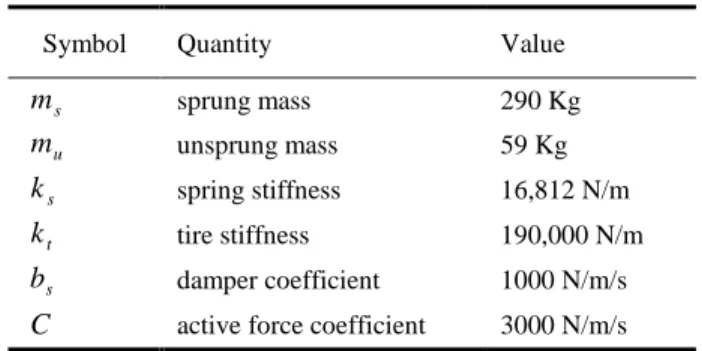
The numerical simulation of equations (4) and (5), using the control law (6), was conducted with parameters from [21] and [22]. These parameters are presented in Table I.

TABLE I

SUSPENSION SIMULATION PARAMETERS

Symbol Quantity Value

s m sprung mass 290 Kg u m unsprung mass 59 Kg s k spring stiffness 16,812 N/m t k tire stiffness 190,000 N/m s b damper coefficient 1000 N/m/s

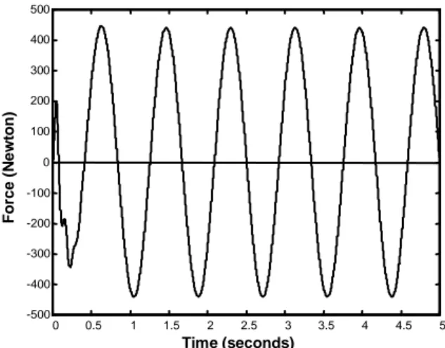
C active force coefficient 3000 N/m/s In the first stage, the actuator forces were investigated in simulation, using a 1.2 Hz frequency and 1-inch amplitude sinusoidal wave as road input disturbance. This amplitude is normally used in published works on this subject [22] and others. The frequency chosen is approximately the sprung mass resonance frequency, also normally used to verify suspension operation.

The actuator parameters for the analyzed case are presented in Table II. Simulation results of the instantaneous force are presented in Fig. 6.

TABLE II

SIMULATION RESULTS FOR A 1.2 HZ FREQUENCY AND 1-INCH AMPLITUDE INPUT DISTURBANCE

Quantity Value Max. Stroke 50 mm Max. Velocity 0.28 m/s Peak Force 450 N R:M.S. Force 295 N Peak Power 65 W R.M.S. Power 37 W

0 0.5 1 1.5 2 2.5 3 3.5 4 4.5 5 -500 -400 -300 -200 -100 0 100 200 300 400 500 Time (seconds) F o rce (N ew to n )

Fig. 6. Active suspension actuator instantaneous force, using a sinusoidal road perturbation of 1.2 Hz frequency and 2.54 cm amplitude.

Although in most situations, the suspension input-disturbance

z

_ris smooth, suspensions must operate in a large spectrum of input disturbance frequency values due to road irregularities, which creates a set of frequencies of distinct amplitudes. The most significant of these frequencies are the resonance frequencies of the sprung and unsprung masses.

ISO 2631 standard gives the acceptable time period exposure of a car passenger to a set of vertical acceleration levels. These vibration levels are set in terms of r.m.s. acceleration values which produce equal 'fatigue-decreased proficiency'. In most situations, exceeding the specified exposure causes noticeable fatigue and may be a cause of a large number of automobile crashes. In the above standard, the r.m.s. acceleration upper bound is taken to be twice the 'fatigue-decreased proficiency' levels. The 'reduced comfort boundary' is assumed to be about one third of standard levels [24].

Automobile drivers automatically avoid the set of 'reduced comfort boundary' frequencies values, simply because they feel uncomfortable, by decreasing or increasing the vehicle’s speed. Consequently, the sprung mass acceleration levels are normally below the levels defined as the 'reduced comfort boundary'. These considerations were used to define the actuator steady state power.

For calculation of the actuator steady state operation upper limits, a numerical simulation of the suspension model was conducted. As model disturbance, a combined signal was used composed of the sum of two sinusoidal waves with different amplitudes and frequencies. These are respectively the sprung and unsprung mass resonance frequencies. The numerical simulation results, conducted for three amplitude sets, are presented in table III. For each frequency-amplitude set the 'reduced comfort boundary' time was found, as shown in table III.

In Fig. 7 the instantaneous force simulation result is presented.

TABLE III

SIMULATION RESULTS FOR THE

REDUCED COMFORT BOUNDARY

Quantity 1.2 Hz / 1.5 cm. 9 Hz/ 0.05 cm. 1.2 Hz / 3.5 cm. 9 Hz/ 0.15 cm. 1.2 Hz / 8.5 cm. 9 Hz/ 0.25 cm. Reduced comfort

time boundary 4 hours 1hour 1 min.

Max. Stroke 32 mm 80 mm 160 mm Peak Force 350 N 900 N 2000 N R.M.S. Force 186 N 451 N 1041 N R.M.S. Power 21 W 139 W 615 W 0 0.5 1 1.5 2 2.5 3 3.5 4 4.5 5 -1000 -800 -600 -400 -200 0 200 400 600 800 1000 Time (seconds) F o rc e ( N e w to n )

Fig. 7. Active suspension actuator instantaneous force, using a set of two sinusoidal road perturbation waves of 1.2 Hz, 3.5 cm amplitude and 9 Hz, 0.15 cm amplitude.

III. ACTUATORDESIGN CONSIDERATIONS

From Tables II and III, and for the suspension parameters presented in Table I, one can define the actuator operation limits for an electromagnetic active suspension. The actuator should be able to produce an r.m.s. force value of 1050 Newton in the steady state. Its stroke should be 160 mm, and the peak velocity is about 1.2 m/s.

A. Maximum dimensions and shape

The actuator must fit in a reasonable space, near the wheel. The available room for the actuator depends on the car design. So it cannot be defined exactly, except for a specific model.

At present, a cylindrical shape seems the most suitable because cars are designed to use hydraulic or pneumatic actuators, and these have a cylindrical shape. Moreover, this shape allows the use of helical sprigs around the actuator, and it can be an advantage for the suspension

design.

The design parameters for an experimental

electromagnetic actuator are presented in Table IV. TABLE IV

ACTUATOR DESIGN PARAMETERS

Quantity Value

Stroke 160 mm

Steady State Force 1000 N

Peak Velocity 1.2 m/s

R.M.S. Power 615 W

Max. Diameter 150 mm

Max. Length 600 mm

B. Actuator lay-out

A cylindrical permanent-magnet linear actuator can be built in two possible configurations: moving magnets or moving coils [19]. However, in an automobile suspension, to define precisely a non-moving part is not possible. In fact, both parts of the actuator are in movement, because one is connected to the sprung mass, and the other to the unsprung mass. However, a moving part can be taken to be the part connected to the unsprung mass.

It is better to put the coils on the sprung mass side because this is the vehicle body side. On the other hand, it is advantageous for suspension performance to have less actuator weight on the unsprung mass side. Developments in high-energy NdFeB magnets allow the construction of reasonable magnetic excitation arrangements [19].

The moving-magnet cylindrical linear actuator can be constructed using radial or axially magnetized permanent magnets.

In the first case, as shown in Fig. 8 a), the magnetic poles are obtained by assembling radial magnetized NdFeB rings on a magnetic-steel rod. In the second case, Fig. 8 b), two opposite-field NdFeB axially magnetized cylinders are assembled sandwiching a magnetic-steel cylinder. The magnetic field crosses the cylinder tops, and then the cylindrical surface.

Fig. 8. Actuator configurations: a) radial magnetization; b) axial magnetization

In both configurations, copper windings are assembled

inside a longitudinally laminated silicon-magnetic-steel slotless armature. The airgap is thus the distance between the poles and the armature, with the copper windings and their electrical insulation almost filling it.

Radially magnetized NdFeB magnets are very expensive compared to axially magnetized magnets. Both configurations were analyzed, using a Finite Elements Analysis (FEA) program.

C. Actuator design analysis

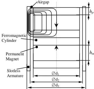
A prototype of a linear permanent magnets cylindrical actuator, using axial magnets configuration was designed. The design analysis of this actuator was made using the magnetic circuit configuration shown in the Fig. 9. All calculations were made neglecting the magnetic flux leakage. Subsequently, all calculations were confirmed using a FEA program and experimental verification.

h

p

h

m d1 d2 d3 Slotless Armature Permanent Magnet Ferromagnetic Cylinder Airgap

Fig. 9. Linear actuator magnetic circuit configuration.

The magnetic flux through the permanent magnet top:

4

2 1

d

B

S

B

_{m m}

=

m

=

(9)

The magnetic flux density on the ferromagnetic cylinder wall: p m p m p

h

d

B

d

h

d

B

S

B

4

4

1 1 2 1 1

=

=

=

(10)

where Bm is the permanent magnet working magnetic flux density medium value.

Chosen the adequate dimensions for it, one can consider equal medium magnetic flux densities on the ferromagnetic cylinder wall, on the top of the ferromagnetic cylinder, and on the top of the permanent magnet. Therefore,

m

B

B

₁

=

(11) From (10) and (11)

4

1

d

h

_p

=

(12) Multiple Finite Elements simulations shown for a NdFeB permanent magnets slotless cylindrical linear actuator, that the maximum magnetic energy density is achieved when the airgap volume under the poles is approximately equal to the permanent magnet volume associated to this poles. For the analysed lay-out:

m p

V

V

2

(13) where Vm is the permanent magnet volume and Vg is the

associated airgap volume. So, from (13)

1

2

1 2

=

+

p m

h

h

d

d

(14)

In the case of a hm=2hp configuration

2

1

2

d

d

=

(15) Taking a magnetic flux value through the armature equal to the magnetic flux value through the ferromagnetic cylinder wall a a p m

d

h

B

d

l

B

₁

=

₂ (16)

where la is the length of the armature wall and Ba the

armature magnetic flux density. From (12) and (16) 2 2 1

4

B

d

d

B

l

a m a

=

(17)

The actuator outside diameter is

a

l

d

d

₃

=

₂

+

2

(18) From (15), (17) and (18)

=

=

+

=

2 2 1 1 2 2 3

4

2

2

d

B

d

B

l

d

d

l

d

d

a m a a (19)

From a given outside actuator diameter d3, solving (19) was calculated the permanent magnet diameter d1. The permanent magnet high was calculated from (12).

+

=

a m

B

B

d

d

4

1

2

3 1 (20)

The actuator Lorenz force produced by a pair of windings and a permanent magnet

g cu

W

i

L

B

F

₂

=

2

r

×

r

(21) where Lcu is the total conductor length of one winding under

the magnetic field, Bg the airgap medium magnetic flux

density and

i

the windings current, calculated from an allowed current density value, taking into account the actuator cooling system.

The actuator final dimensions were calculated from (22)

W A W

F

F

n

2

2

(22) where FA is the actuator steady state final force and

n

W the total number of windings under magnetic field.

The coefficient K was calculated from (23)

g W cu

n

B

L

K

=

(23) Since the actuator is cylindrical, it is axisymmetric and seems that the analysis could be conducted on two-dimensional plane. However, was chosen to use tri-dimensional FEA calculations, because the magnetic flux density value varies significantly along the actuator radius. The flux plots obtained from this analysis are presented in the Figs 10 and 11, related to a pair of poles and one winding, for a 100mm-outside-diameter actuator.

Fig. 10. Flux plot of an actuator pair of poles, using radially magnetized NdFeB permanent magnets.

Fig. 11. Flux plot of an actuator pair of poles, using axially magnetized NdFeB permanent magnets.

Table V presents the parameters used in the calculations and several values obtained from the FEA results.

TABLE V

FINITE ELEMENTS ACTUATOR ANALYSIS

Quantity Radial magnetization Axial magnetization Actuator diameter 100 mm 100 mm Airgap length 11 mm 13 mm

Average flux density

near the pole 0.47 T 0.68 T

Average flux density

near the armature 0.29 T 0.41 T

One-pole flux 3.04 mWb 4.15 mWb

Non-moving part

weight 0.95 Kg per coil 0.85 Kg per coil Moving part weight 0.9 Kg per pole 1.25 kg per pole One-coil current 1025 At 1226 At Force produced 88 N per pole 148 N per pole

IV. PROTOTYPE DESCRIPTION

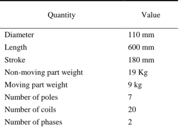
Based on the above analysis and calculations, a linear actuator was built using axially magnetized NdFeB cylindrical permanent magnets. The experimental actuator parameters are presented in Table VI.

TABLE VI

EXPERIMENTAL ACTUATOR PARAMETERS

Quantity Value

Diameter 110 mm

Length 600 mm

Stroke 180 mm

Non-moving part weight 19 Kg

Moving part weight 9 kg

Number of poles 7

Number of coils 20

Number of phases 2

An actuator with these dimensions can fit in the available space near the wheel. However, these values are high, and they are larger than an equivalent hydraulic actuator. A further development in the actuator cooling system could significantly reduce the dimension and weight values presented.

A photograph of the actuator prototype is presented in Fig. 12. Here, the actuator is mounted in a steel structure, to measure the produced forces. Figure 13 shows the

laboratory workbench constructed for the evaluation of the actuator as an electromagnetic suspension.

Fig. 12. Actuator prototype.

Fig. 13. Actuator prototype and partial view of the workbench.

A. Power Electronics Converter

A converter composed of two IGBT full bridges is used to control the current values in the actuator phases. In figure 14 the converter layout is shown. The inductances represented in the figure are the actuator phase inductances added to external inductances, in order to limit the current gradient. In the prototype L1=L2=5 mH.

The semiconductor switches work in accordance with a sliding mode control law [23]. So, the voltage output value

of each phase is given by (24). The commutation frequency maximum of each IGBT can be calculated by (25). For a set of 50V supply voltage and i=500mA, a maximum of 5 kHz commutation frequency was found.

< > + = i i U i i U t U if if ) ( (24) iL U f = 4 max max (25) Actuator S1 S3 S2 S4 S5 S6 S7 S8 L1 L2 Udc

Fig. 14. Power electronics converter layout.

B. Phase Current Control

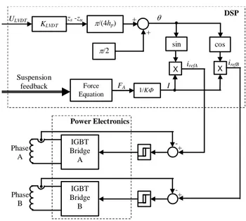
The finite elements analysis shows that the radial magnetic induction in the windings along the actuator has a sinusoidal variation. So, the currents should also have a sinusoidal variation, in order to ensure an optimal linear relation between the current and the force. As it is a two-phase winding system, the current of one two-phase must be shifted by a arc angle of /2 relative to the other phase.

The current should be dependent on the position of the poles, relative to the windings. An LVDT sensor was used to measure the distance between the sprung and unsprung masses. This distance is calculated from (26), where ULVDT

is the sensor output voltage value and KLVDT is a constant

coefficient. The equivalent position angle is obtained from (27), where h is the pole length. A phase current control functional diagram is shown in figure 15.

LVDT LVDT u s z U K z )= ( (26) 2 2 + = h K U_{LVDT LVDT} (27) X I FA Force Equation 1/K Suspension feedback cos sin zs -zu ULVDT KLVDT DSP IGBT Bridge A Phase A + -Power Electronics IGBT Bridge B Phase B + -irefA irefB /(4hp) /2 + + X

Fig. 15. Phase current control functional diagram.

In Fig. 16 the experimental results of the force values produced by the actuator prototype versus the current per phase are shown.

0 200 400 600 800 1000 1200 0 5 10 15 20 25 30

Current per phase (Ampere)

F o rc e ( Ne w to n )

Fig. 16. Force produced by the actuator prototype, versus the current per phase.

V. EXPERIMENTAL RESULTS

The input disturbance is produced with an appropriate workbench drum surface, Figure 13. The input obtained is an almost sinusoidal perturbation with a frequency value of 3.28 Hz and amplitude equal to 8 mm. However, as presented in Fig. 17, the obtained disturbance amplitude spectrum also shows some frequency components.

Experimental results of the linear actuator working as a passive suspension system are shown in Figures 18 and 19. In this simpler system the actuator is working as an electric generator. Each actuator phase is connected to an external power resistor. No power electronics are connected. In this configuration, with the resistors connected to the armature,

the system is equivalent to a 1350 N/m/s damping coefficient.

The sprung mass acceleration presented in figure 15 shows that the actuator can operate as a passive suspension, damping the oscillations caused by the ground irregularities. The obtained sprung mass acceleration peak values are in agreement with what is expected for a passive suspension.

Figure 16 shows the evolution of the force produced by the actuator. In general, the experimental results obtained validate the simulation model used. The experiments also show the capability and applicability of this kind of linear permanent magnet actuator for automotive suspension systems. 0 5 10 15 20 25 30 35 40 0 1 2 3 4 5 6 7 8x 10 -3 Frequency (Hz) A m p li tu d e ( m )

Fig. 17. Disturbance amplitude spectrum obtained from FFT analysis of the workbench irregularities profile.

0 0.1 0.2 0.3 0.4 0.5 0.6 0.7 0.8 0.9 1 -0.4 -0.3 -0.2 -0.1 0 0.1 0.2 0.3 0.4 Time (seconds) A c e le ra ti o n ( g 's ) Experimental Simulation

Fig. 18. Sprung mass acceleration.

0 0.1 0.2 0.3 0.4 0.5 0.6 0.7 0.8 0.9 1 -300 -200 -100 0 100 200 300 400 Time (seconds) F o rc e ( N e w to n ) Experimental Simulation

Fig. 19. Force produced by the actuator.

VI. CONCLUSIONS

The analysis and the experimental results show that it is possible to build an electromagnetic actuator, suitable for application in an automobile electromagnetic suspension. It is shown that the force values produced by the actuator are suitable for the proposed application. The constructed actuator is oil-free and does not need any kind of hydraulic system.

Although the dimensions and the weight are suitable, these values are larger than an equivalent hydraulic actuator. However, further development in the actuator cooling system could significantly reduce the dimension and weight values presented. For instance, the performance of a water-cooled actuator should be investigated.

The utilization of this electrical drive system in the automobile suspensions allows a relatively easy implementation of an active control suspension law. Furthermore, the application of other control laws allowing improvements in the automotive suspension performance becomes possible.

ACKNOWLEDGMENT

Acknowledgment are due to the authors of the finite elements analysis program Finite Element Method Magnetic (FEMM) and to all colleagues involved in the project "Electromagnetic Vehicle Suspensions" funded by the PRAXIS Program and Portuguese FCT.

REFERENCES

[1] A.P. Yankowski and A. Klausner, "Electromagnetic Shock Absorber", U.S. Patent No. 3,941,402, 1976.

[2] C. Theodore and J.A. Ross, "Suspension Dampening for a Surface Support Vehicle by Magnetic Means", U.S. Patent No. 3,842,753, 1974.

[3] W.C. Kruckemeyer, H.C. Buchanan Jr. and W.V. Fannin, "Rotational Actuator for Vehicle Suspension Damper", U.S. Patent No.

4,644,200, 1987.

[4] B.V. Murty, "Electric, Variable Damping Vehicle Suspension", U.S.

Patent No. 4,815,575, 1989.

[5] B.V. Murty and R.R. Henry, "Active Vehicle Suspension with Brushless Dynamoelectric Actuator", U.S. Patent No. 5,091,679, 1992.

[6] R.R. Henry, M.A. Applebee and B. V. Murty, "Full Car Semi-Active Suspension Control Based on Quarter Car Control", U.S. Patent No.

5475596, 1995.

[7] D.A. Weeks, D.A. Bresie, J.H. Beno and A.M. Guenin, "The Design of an Electromagnetic Linear Actuator for an Active Suspension", in

Proc. of SAE Steering and Suspension Technology Symposium,

Detroit, USA, 1999.

[8] J.H. Beno, D.A. Weeks and W.F. Weldon, "Constant Force Suspension, Near Constant Force Suspension, and Associated Control Algorithms" U.S. Patent No. 5,999,868, 1999.

[9] Z. Kurtzman, "Electromagnetic Strut Assembly", European Patent

Application No. EP 0 343 809 A2, 1989.

[10] K.O. Stuart, "Electromagnetic Actuator", U.S. Patent No. 4,912,343, 1990.

[11] K.O. Stuart and D.C. Bulgatz, "Electromagnetic Actuator", U.S.

Patent No. 5,187,398, 1993.

[12] P. Denne "Motion Control Systems", International Patent No. WO

95/16253, 1995.

[13] J.-J. Charaudeau, D. Laurent and J.-L. Linda, "Suspension Device Comprising a Spring Corrector", U.S. Patent No. 6,161,844, 2000.

[14] I. Martins, J. Esteves and F. Pina da Silva, "Energy Recovery from an Electrical Suspension for EV", in Proc. Electric Vehicle

Symposium EVS-15, Brussels, 1998.

[15] I. Martins, J. Esteves, F. Pina da Silva and P. Verdelho, "Electromagnetic Hybrid Active-Passive Vehicle Suspension System", in Proc. IEEE Vehicular Technology Conference, VTC’99, Houston, U.S.A.

[16] I. Martins, J. Esteves, F. Pina da Silva and A. Tomé, "Automobile Suspensions Using Electromagnetic Linear Actuators", in Proc. IFAC

Conference Mechatronics 2000, Elsevier Science, 2001.

[17] J.G.Kassakian, H.-C. Wolf, J.M. Miller and C.J. Hurton, "Automotive Electrical Systems Circa 2005," in IEEE Spectrum, August, 1996.

[18] K.E. Graves, P.G. Iovenitti, and D. Toncich, "Electromagnetic Regenerative Damping in Vehicle Suspension Systems", in Journal

of Vehicle Design, Vol. 24, Nos 2/3, 2000.

[19] B. Lequesne, "Permanent Magnet Linear Motors for Short Strokes",

IEEE Transactions on Industry Applications, Vol. 32, No 1, 1995.

[20] T.D. Gillespie, "Fundamentals of Vehicle Dynamics", Society of Automobile Engineers, ISBN 1-56091-199-9, 1992.

[21] R. Rajamani, and J.K. Hedrick, "Adaptive Observers for Active Automotive Suspensions: Theory and Experiment", IEEE Transactions on Control Systems Technology, Vol. 3, 1995.

[22] A. Alleyne, and J.K. Hedrick, "Nonlinear Adaptive Control of Active Suspensions", IEEE Transactions on Control Systems Technology, Vol. 3, No 1, 1995.

[23] V. Utkin, J. Guldner and J. Shi, "Sliding Mode Control in

Electromechanical Systems", Taylor & Francis, London. ISBN

0-7484-0116-4, 1999.

[24] J.T. Broch, "Mechanical Vibration and Shock Measurements", Brüel & Kjaer, Denmark, ISBN 87 87355 36 1, 1984..