A new method to
map groundwater
potential at a village
scale, based on a
comprehensive
borehole database.
An application to
Sikasso, Republic
of Mali.
Ana Carolina Gonçalves Delgado
Mestrado em Geologia
Departamento de Geociências, Ambiente e Ordenamento de Território 2017/2018
Orientador
Jorge Espinha Marques, Professor Auxiliar, Faculdade de Ciências da Universidade do Porto
Coorientador
Pedro Martinez Santos, Professor Titular, Facultad de Ciencias Geológicas, Universidad Complutense de Madrid
Todas as correções determinadas pelo júri, e só essas, foram efetuadas. O Presidente do Júri,
Acknowledgements
I would like to express my deep sense of gratitude to Prof. Pedro Martinez Santos for the invaluable support, continuous guidance and for providing me the opportunity to embark on this project which started in Spain.
To Prof. Jorge Espinha Marques I would also like to thank for his valuable advice and excellent guidance trough the development of this dissertation.
I am thankful to all the people who helped me directly or indirectly to complete this thesis. Last but not the least I would like to thank my family for all the support provided not only during the writing of the thesis but also throughout all my time in University.
Abstract
in portugueseO principal objetivo da presente Dissertação foi a elaboração de um mapa de potencial das águas subterrâneas para a região de Sikasso, na República do Mali, com base nos mesmos parâmetros utilizados num estudo prévio, mas para todo o país e uma posterior comparação e análise dos mesmos, de forma a clarificar a importância e relevância deste tipo de estudo a escalas mais localizadas. Para tal, criou-se uma base de dados com os poços tradicionais e os furos existentes em Sikasso e sua respetiva informação. Para tratamento desta mesma base de dados e para a elaboração de mapas temáticos e de potencial das águas subterrâneas utilizou-se o software QGIS.
A tese foi desenvolvida, numa fase inicial, em Espanha, entre setembro de 2017 e janeiro de 2018, em colaboração com a Universidad Complutese de Madrid (inserida no programa Erasmus +) e terminada em Portugal, na Universidade do Porto, a setembro de 2018.
Abstract
in EnglishThe main goal of this thesis was the elaboration of a groundwater potential map for the Sikasso region, in Republic of Mali, based in the same parameters used in a previous study but for all country, and a later comparison and analyses of them, aiming to clarify the importance and relevance of this type of study at smaller scales. For that, a database was created with the location of the traditional wells and boreholes and its information. To treat this database and develop the thematic and groundwater potential maps the open source software QGIS was used.
This thesis was developed initially in Spain, between September 2017 and January 2018, in colaboration with Universidad Complutense de Madrid (as part of an Erasmus+ program) and was completed in Portugal, in Porto University, in September 2018.
Table of contents
Acknowledgements ... 3 Abstract in portuguese ... 4 Abstract in English ... 5 Table of contents ... 6 List of figures ... 7 List of tables ... 9 1.Introduction ... 10 2.Study area ... 13 2.1 Climate ... 13 2.2 Geology ... 15 2.3 Hydrogeology ... 22 2.4 Borehole database ... 25 3. Hydrogeological parameters ... 264. Methods and procedures ... 27
4.1 Database ... 27
4.2 QGIS analyses ... 28
5. Results and discussion ... 30
7. Bibliography ... 43
8. Appendix ... 47
List of figures
Figure 1-Average annual rainfall in Mali between 1971 and 2000 . ... 14Figure 2-Sikasso precipitation (mm) ... 14
Figure 3-Mali´s main geological units ... 16
Figure 4- Yafolila, Morila and Syama belts ... 17
Figure 5-Geological simplified from Sikasso. Modified from ... 19
Figure 6-Mali´s aquifers. ... 23
Figure 7- Geographical location of the Klela Basin ... 24
Figure 8-Long-term annual recharge in the Klela Basin ... 24
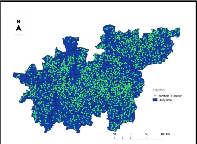
Figure 9-Location of the boreholes in the study area. ... 26
Figure 10-Borehole success rate thematic map. ... 30
Figure 11-Borehole yield thematic map. ... 31
Figure 12-Borehole depth thematic map. ... 33
Figure 13-Electrical conductivity thematic map. ... 34
Figure 14-Location of the highest electrical conductivity value. ... 35
Figure 15-Borehole success rate thematic map based on the new breaks. ... 36
Figure 17-Commune scale and village scale groundwater potential maps. Commune
scale map adapted from ... 38
Figure 18-Areas with not enough data. ... 39
Figure 19-A-Groundwater potential map and B- Geological map from the western part of Sikasso adapted from (Sandy, 2017). ... 40
Figure 20-Database sheet provided by DNH. ... 47
Figure 21-Part of the attribute table organized database. ... 48
Figure 22-Sikasso and study area (Sikasso + borders) ... 49
Figure 23-Borehole success rate grid produced with Surfer 11, with the kriging method. ... 56
List of tables
Table 1-Mali´s main geological units ... 15 Table 2-Values for each defined category and parameters. ... 29
10
1.Introduction
Africa is the second driest continent in the world and many Africans still suffer from water shortages during the year (WWF, 1986).
Mali is one of the hottest African countries, its land is stretching far into the Sahara Desert and the precipitation levels through the country are very low. There are several regions in sub Saharan Africa where rainfall is absent for several months each year and groundwater resources are widely relied upon. It is estimated that about 200 million people uses water from African aquifers for their daily life needs (Martínez-Santos et al., 2017). Most of the Malians live in the south and rely on farming for a living.
It is still possible to see a lot of poverty in the country and finding water is a constant concern among the people living there (Mali, WaterAid Global, n.d). Adding to this fact, several studies say that throughout the years population tends to grow and so the water needs. Groundwater is a crucial resource in the drier parts of Mali and in the future more water will be taken from the aquifers and at faster rates. Another relevant aspect to be considered is the climate change that suggests a less reliable rainfall in Sikasso for the next years (USGS, 2012).
Nowadays there are two different main ways used in Mali for the extraction of water. One of them is from boreholes owned and operated mostly by communities where groundwater is supplied to the population by means of standpipes or hand pumps. The other way is known to be less efficient even though it is very commonly used. It consists on private domestic wells that were dug by people. They tend to be more vulnerable to drying up periodically and to contamination but with them people can avoid queuing at community water points and walking the distance (Martínez-Santos et al., 2017).
Mali is not considered a water-short country since renewable water resources range between 3,500 m3 and 7,000 m3 per person, which is way above the 1,700 m3/ person threshold for water poverty. It is important to understand that these values represent an average form all the country and even though there are some places with big quantities of water (increasing that average), there are many other widespread areas that are at or below threshold of water poverty. Millions of people and animals have perished in Mali over the past half century due to drought-related catastrophes. (Murray-Rust, 2013). Considering the previously described evidences, the importance of groundwater studies in Mali becomes clear. It is fundamental to understand as deeply as possible how much
11 groundwater is stored in the country, how well its distributed and where and how it should be taken from, in the most sustainable way, in order to alleviate poverty and make sustainable use of a scare resource. Mapping the groundwater potential can be a very good contribution to increase the knowledge of a certain area and understand what places are more likely to have groundwater.
Over the past few years the process of mapping groundwater potential has been developing. The term “groundwater potential” denotes the amount of groundwater available in a certain area and it is a function of several hydrogeological and hydrological factors that can be direct or indirect (Jha et al., 2010). The use of technics such as digital elevation models (DEM) and satellite imagery is being explored and stared to be used more often as a source of data and as an alternative to the traditional field surveys (which are less efficient in terms of time and resources, especially in the developing countries). Geographic Information System (GIS) is a computer system built to store, capture, manipulate, analyse, manage, and display all kinds of spatial or geographical data. It is not only a time-effective way to treat the information as it is also a cheap way to do it and due to these great advantages, many hydrogeologists have been using it to map groundwater potential these days. In most cases ArcGIS and QGIS are the geographic information system softwares used to treat the available data which, according to the existing literature, comes mainly from indirect parameters such as lithology, lineaments, drainage, slope, topography, land use, land cover, etc. (Balamurugan et al., 2016; Ganapurm et al., 2008; Hussein et al., 2016; Krishna-Gumma et al., 2012; Mondal, S, 2011; Rahmati et al., 2015; Sternberg et al., 2015; Yeh et al., 2016.). There are many ways in which these indicators can help us understand how the water behaves under the ground, for example, a very rough terrain with many scarps and ridges is most likely to have a poor groundwater potential. Although it is possible to use the indirect indicators mentioned above to produce groundwater potential maps the results obtained from the direct data taken from the boreholes are, in theory, more reliable once there was a direct approach to the object of study and not only suppositions from what´s above and can be seen with our eyes.
In the Republic of Mali there are over 800 000 known traditional wells and 25 000 boreholes spread around the country. Using this available information, it was possible to map the groundwater potential in Mali at a commune scale, based on direct parameters (borehole depth, yield, success rate, electrical conductivity, etc.) and using the software QGIS. (Díaz-Alcaide et al., 2017).
12 The present work has two main purposes. Firstly, the development of a village scale groundwater potential map of the Sikasso region, based on the previously described large borehole database. The goal is to develop the map using the same procedures and direct indicators used to create the commune scale existing one. The second main goal is to compare both maps (village and commune scale), understand the differences between them and whether it is relevant or not to have a more detailed map.
13
2.Study area
2.1 Climate
Republic of Mali is a landlocked West African country with already more than 19 million people, a number that, according to several studies, will grow in the upcoming years (Mali Population, 2018). In terms of size, an area of 1,240,278 square kilometers makes it the 8th largest African country (CIA, 2011). It is known to have a very particular climate due to its location and it is influenced by the Inter-Tropical Conversion Zone (ITCZ) which means being affected by two opposite wind directions, those coming from the ocean and the warmer ones from the Sahara region. This condition makes the country have a dry season for a period between 6 months (in the south) and 9 months (in the north) and a wet season of 3 to 4 months between June and October (mostly in the south of the country) (NCEA, 2015). This phenomenon is named West African Monsoon, it also occurs in other West African regions and it is a coupled atmosphere-ocean-land system characterized by summer rainfall over continent and a prolonged abnormal winter period of low or even any rainfall (NTUN, 2015).
The surface drainage network of Mali is controlled by two main rivers, Niger and Senegal and the distinct climate divides the country into four different zones. From north to south it starts with the Saharan climate with less than 200 mm of precipitation per year, followed by Sahel climate with precipitation between 200 and 600 per year and then the Sudanese and Sudano-Guinean climates with 600 to 1000 and over 1000 mm respectively (NCEA, 2015). The following climatic map, from Figure 1, shows the average annual rainfall in the country between the years 1971 and 2000.
14 Sikasso is affected by the Sudano-Guinean climate and its annual precipitation is represented in the climograph from Figure 2, showing how irregularly the rainfall is distributed across the year.
Figure 1-Average annual rainfall in Mali between 1971 and 2000 (Modified from Diallo et al., 2011).
15 Through the last years climate changes are already being felt in Mali and are expected to continue happening. These have been influencing the variability of rainfall, the magnitude of extreme weather conditions and increasing local temperatures which leads to an increase of conflicts between Malians due to a steady relocation of agricultural, fishing and livestock keeping activities southwards where the population is much higher. Sikasso is a region in southern Mali considered to be the breadbasket of the country providing a substantial amount of food supplies and even though it has remained stable so far, this region cannot be considered immune from the impacts of conflicts in north and central Mali, given the fragility of the governance in the country, as well as from the pressures of environmental degradation, natural resources stress and climate change impacts (Mitra, 2017).
2.2 Geology
The global geology of Mali can be characterized by two distinct main structures. In the eastern part of the country the Tuareg shield was brought together to the end of Precambrian, between 600 and 550 million years ago. In the west side the West African Craton is the dominant structure with around 1800 millions of years (Kusnir I, 1999). The main geological units that can be found in Mali are organized chronologically in the following table (table 1):
Precambrian Birimian crystalline basement.
Lower Cambrian to Paleozoic Sandstones and metamorphosed clays (“pelits”).
Permian Dolorite intrusions.
Mesozoic Mixed continental sediments of the “continental intercalair” formation.
Upper Cretaceous to Eocene Marine sediments.
Pliocene “Continental terminal” sedimentary formation.
Quaternary Superficial deposits.
16 Looking closely to the study area (Sikasso region) a clear geological division is notorious. In the east part the sedimentary formations (mostly sandstones, but with some argillaceous and carbonate horizons) of the lower Precambrian prevail, as in the west part of the region, on the other hand, the geological units are mainly granites and metamorphic rocks from the Precambrian basement (Figure 3).
The Birimian greenstone belts of the West African Craton are known to be able to host accumulations of gold. Based on their favorable Paleoproterozoic structure and geology, Sikasso has several places that are considered prospective for orogenic gold style mineralization.
Due to the limited outcrop and the general lack of drilling, southern Mali´s geology is not known very deeply. The existing paper where most of the information about Sikasso is described in is a technical report on the Sikasso property. It focuses mainly on some specific areas and shows its geology with bigger detail, which is helpful to correlate and understand all general Sikasso´s geology (Sandy, 2017).
17 According to that same report there are three main Birimian Eburnean litho-structural units in Sikasso. The NS striking Birimian dacitic to andesitic volaco-sedimentay series of the Yanfolila, Kalana and Bagoé basins (Yafolila, Morila and Syama greenstone belts) is one of them, another one is a suite of granite to monzogranitic units which intrude the Birimian volcano-sedimentary units and last the late dioritic to granodioritic intrusives occurring as plugs and dykes (Jones et al., 2016).
The Yafolila, Morila and Syama belts are represented in the following picture (Figure 4):
18 The Yanfolila belt is located along the border with Guinea and is bisected into western and eastern segments by the regional Siekerole Shear Zone. It is comprised of a suite of arc-related volcanic units (the Nani Volcanic Formation) and reworked greywacke sequences. This Nani Volcanic Formation is composed by tholeiitic basalts and basaltic andesites and deformed porphyritic rhyolitic to dacitic lavas, pyroclastic flows and breccias (Parra-Avila et al., 2016).
The Morila Belt occurs within the major granitic intrusive complex of the Bougouni region and its domain contains the Massigui and Doubakoro TTG granites.
The Birimian units, in this region, are comprised of basalt to basaltic-andesite lavas locally alternating with volcano-sedimentary units. All have undergone amphibolite grade metamorphism (Parra-Avila et al., 2016).
The Syama Belt is separated from the Morila belt by the regional Benafin Shear Zone and is situated along the Mali-Burkina Faso border. It is lithologically similar to the Yanfolila belt being characterized by greywackes and argillites interbedded with a sequence of basalts and andesites (Olson et al., 1992). Structurally, the Syama belt is entirely segmented, strongly folded and frequently overturned. Other than that, the regional plutonism occurred during the Paleoproterozoic (Ballo et al., 2016. Parra-Avila et al., 2016).
A simplified geological map of Sikasso (from the west side) was taken from (Sandy, M, 2017) and modified. The five selected areas in the map (A, B, C, D and E) were then described with more detail (Figure 5).
19
20 The detailed information about the geology of each of the following areas can be very interesting tools to understand more deeply about the groundwater in those places as they are representative of regional-scale conditions.
Areas A and B
Due to the lack of exploration and the dearth of outcrop, the geology of the areas is mainly based on limited surface geology and interpretation of the airborne radiometric and magnetic surveys.
The area A is located in the Yanfolila-Kalana-Manakoro basin and the main lithology found is the Birimian volcano-sedimentary units with minor syn- and pos- tectonic granites. They occur as isolated and small massifs and a cover sequence of colluvium and alluvium.
The area has suffered extensive lateritization and intense weathering and the Birimian series are mainly comprised of siliciclastic sediments. The granitic bodies found are typically fine-grained monzogranitic to granodioritic in composition with development of some microgranites (Sandy, 2017).
The area B is located between the Yanfolila-Kalana-Manankoro and the Kangaba basins and it´s lithology is composed mainly of Birimian volcano-sedimentary units intruded by elongate granitoid massifs. The volcano-sedimentary units have fine to coarse grained siliciclastic sediments alternating with greywackes, siliceous greywackes and small intercalations of volcanic lithologies rich in biotite and feldspar.
Both locations are most likely to belong to the Jurassic age, they are cut by a late, east-west trending dyke, regionally extensive and probably composed of dolerite. The structures in the area mainly NE, NNE, NNW and EW and are related to the Yafolila major fault which forms a NE structural corridor with secondary or splay structures orienter NNW and NNE (Diallo and Diakité, 2011b. Diallo et al., 2017b).
Areas C and D
The geology of those areas is also poorly previously described due to the lack of drilling and poor exposure.
21 Like the other two places, they are both located in the Yafolila-Kalana-Manankoro basins but at the eastern edge of the Siekerele Shear Zone.
Lithologies are composed primarily of Birimian volcano-sedimentary units of fine to coarse grained siliciclastic sediments alternating with minor mafic and felsic volcanic rocks and volcaniclastic units (Diallo et al., 2017c).
The sequence was intruded by a series of biotite-bearing monzogranites, porphyritic granites and microgranites, which were intruded by fine-grained granite and granodiorite. Corresponding with the regional foliation, the smaller intrusions have mostly a northeast trend. In the southern part there is a discontinuous east-west trending mafic dyke intruding. This dyke is not a regional scale feature like the other dyke cutting the areas A and B.
Structurally, the known faults have a northeast trend confirmed by the magnetic survey data and a series of northwest trending faults were also identified.
Area E
This area is situated in the Syama Belt of the granitic dominated eastern domain (Ballo et al., 2016).
There are different interpretations about its geology. According to the BRGM (Feybesse et al., 2006b) the underlying geology is dominantly granitic, with a north-south trending intrusion of mafic rock (gabbro or basalt, metamorphosed to amphiblite/metabasite) in the southern part whereas in the western part there is a small amount of mafic volcaniclastic rock. On the other hand, The WAXI (AMIRA, 2013) interpreted the underlying geology as composed totally of granite, except for two east-west trending mafic intrusions.
Interpretation of the detailed airborne geophysical survey, in the same place, by SERM SARL in 2016 (Diallo et al., 2016b) suggests that the area might be underlain by a sequence of northeast-trending metagreywackes and shales which have been intruded by, or juxtaposed to, granites and granodiorite, suggesting also that the felsic intrusive rocks were later intruded by mafic rocks.
22
2.3 Hydrogeology
About Sikasso´s hydrogeology most of the information found was provided by the Département de la Coopération Technique pour le Développement (DHN, 2010) where a description of Mali´s aquifers was available.
This work divided the country into nine different major systems (Figure 6), which can be distinguished depending on the type of deposit. Four of them with intergranular porosity and the other five with fissured porosity.
• The intergranular porosity deposits, associated with formations with little or non-consolidation, can be find in the large sedimentary basins of the secondary Quaternary (north-east of Koulikoro, centre and north of Segou, centre and north of Mopti, large parts of Timbuktu and Gao).
• The fissured porosity deposits correspond to semi continuous or totally discontinuous cracked aquifers. This type of aquifers can be found in crystalline formations, crystallophyllian and sedimentary from the primary Precambrian. They occur mainly occur mainly in the south (Sikasso), west (Kayes), center (Koulikoro except its north-east part, Segou in its southern part, Mopti in its southern part) and to the east of the country (the southern region of Gao region and most of the Kidal in the massifs of Adrar and Iforas).
Deep aquifers are usually surrounded by shallow aquifers, lateritic alteration formations in flat surfaces in alluvial and colluvial deposits, plains and valley bottoms. Depending on the thickness, precipitation and geomorphology, superficial aquifers are either semi-continuous or in hydraulic connection with aquifers deep or dissemi-continuous in perched position (WWAP, 2006).
Both types found in Sikasso are from the fissured porosity type (discontinuous) and the groundwater units that constitute this region are the Infracambrian tabular (with sandstones and schist) in the eastern part and the granitic and metamorphic basement (with laterite, clay, sand and gravel) in the western one (Martínez-Santos et al., 2017).
23
Figure 6-Aquifers of Mali (Díaz-Alcaíde et al 2017).
There is not much available information about Sikasso´s hydrogeology and the few things that can be found are unevenly distributed. There are, although, some punctual studies that can be important to understand the hydrogeology of the region.
To understand the importance of climate changes on groundwater resources a study was developed in the Klela Basin (East of Sikasso) (Figure 7) in which a simulation of the groundwater dynamics was done. MODFLOW was the program used for that and the results of the simulation show a decrease in groundwater levels over time. The sandstone aquifer was simulated in steady transient conditions and the recharge decreases from 1970 to 2050 and several droughts occur from 2030 to 2037 as it is possible to see in the graph from Figure 8 (Toure et al., 2016).
24
Figure 7- Geographical location of the Klela Basin (Toure et al., 2016)
25
2.4 Borehole database
The base tool of this study is a database provided by the “Direction Nationale de l´Hydraulique” (DNH, 2010). It includes information on parameters such as borehole yield, average depth, success rate, electrical conductivity, etc. All the available borehole information of Sikasso and its borders was typed up to an excel file together with its location coordinates taken from a shapefile available at the United Nations Office for the Coordination of the Humanitarian Affairs website (OCHA, 2018).
The database used on this study is constituted by 7031 spatially distributed boreholes. Initially, the study area included only the Sikasso region, but it was later extended, ended up including also the border villages from Segou and Kolikouro. The reason for this expansion of the area lies on the fact that country divisions do not translate the groundwater reality and even though the focus is the Sikasso region the results obtained are more reliable and closer to reality if a bigger area is considered.
From all the boreholes used 82% are called successful as the other 18% unsuccessful. Typically, a yield in excess of 500 to 1000 liters per hour is enough to sustain a hand pump and therefore considered positive even though there is a small quantity of water available. Looking at these percentages it is possible to note that in the big majority of those boreholes enough water was found to fulfil a specific need, such as small-scale irrigation or domestic consumption. Only in a minority (18%) no water was found, or not enough.
The following map (Figure 9) shows the location of all the exiting boreholes in the study area. This translates into 2116 different places as borehole data is disaggregated at the village scale, but the database does not provide the specific coordinates of each borehole. Hence, a dot may represent several boreholes.
It is possible to notice that the boreholes do not have the same distance between them meaning that some areas are more represented than others. This is an important fact to be considered in the results analyses.
26
3. Hydrogeological parameters
The final database used in this work includes several different fields such as the number of negative and positive boreholes in each location, as well as the average borehole success rate, the yield, depth, static level and electric conductivity. From all this information the parameters used to produce the thematic maps were only the following, and the same ones used in the previous commune scale work (Martínez-Santos et al., 2017).
The borehole success rate (%): The borehole success rate measures how likely groundwater is to be found in a certain place and can vary a lot depending on the characteristics of the ground. If it is a fissured porosity kind of region it is more likely that there´s a bigger range between the values as they will be much higher in fractured or weathering zones making the information taken from those values very relevant. On the other hand, in regions where there is predominance of intergranular porosity the
27 boreholes success rate will probably be much more equal (with similar values all over the area).
Considering Sikasso´s geology the borehole success rate values are supposed to change more in the western part of the commune.
The borehole yield (m3/h): This parameter is, by definition, the volume of water that can
be abstracted from a borehole providing a good idea of how productive the aquifer is. The borehole depth (m): The borehole depth provides information about the drilling costs, the deeper the borehole, the more expensive it is. It also shoes how deep a borehole needs to be to supply enough quantities of water.
Electrical conductivity (μS/cm): The electrical conductivity measures the ability of a solution to carry an electric current. The more ionic solutes that are dissolved in the water the greater its electrical conductivity will be. This parameter alone cannot tell us whether the water is good for consumption or not, but it is a good indicator of the water quality and can identify some unsuitable aquifers (those with very high values).
4. Methods and procedures
Through the development of this work two distinct main phases were necessary. Firstly, the creation of a database with all the information available and required for the present study and secondly the QGIS analyses of the previously organized data.
4.1 Database
The creation of the database is the base of all the work and its quality will compromise the later results, therefore it is important to make it carefully.
The available necessary information was provided by the “Direction Nationale de l´Hydraulique” (DNH, 2010) as printed sheets and in order to work with the QGIS program it was necessary to type up all the information to a digital format. An excel file was initially created and later exported to an attribute table. During this process it was necessary to associate the information provided with the correspondent locations
28 available in the United Nations Office for the Coordination of the Humanitarian Affairs website (OCHA, 2018).
4.2 QGIS analyses
QGIS 2.18.13 and the application Surfer 11 from the Golden Software were used to turn all the available borehole´s information into thematic maps. QGIS is a free open-source cross-platform desktop that supports viewing, editing and analysis of geospatial data. Surfer 11 was used to develop the base grids that were later used in QGIS to produce the thematic maps. For the creation of the mentioned grids an interpolation method called kriging was selected in order to estimate values at unknown points based on the known ones. Among many different possibilities the kriging method was chosen because a kriged estimate is a weighted linear combination of the known sample values around a certain unknown point to be estimated and kriging assumes that the direction or distance between sample points translates into a spatial correlation that can be used to explain surface variations. This procedure generates an estimated surface based on z-values and it is appropriate to be used when there is a spatially correlated distance or directional bias in the data. This makes kriging the best method to be used in this case and it is also why it is often used in soil science and geology (“Gis Resources”, n.d.).
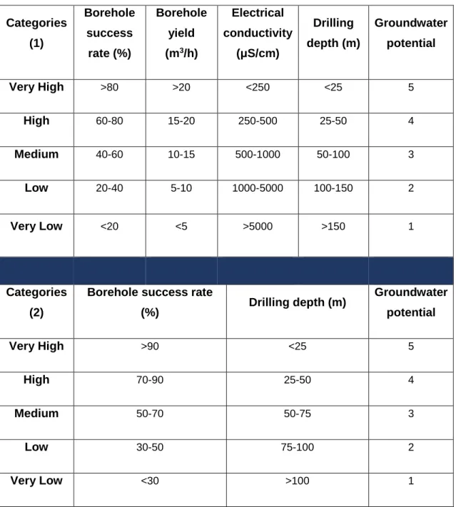
The thematic maps were created based on five different settled categories for each of the four key variables. A scale from 1 to 5 was defined, where 5 corresponds to a very high groundwater potential indicator and 1 to a very low.
The breaks between the categories were based in different criteria for each variable to make the scores as meaningful as possible. For this work the same breaks used by Martinez-Santos were kept (Categories 1 in Table 2) with some exceptions where small changes in the breaks´ values were done (Categories 2 in Table 2), in order to make the results more meaningful and appropriate to the different smaller used scale. Borehole depth and yield were classified based on Jenks´frequency analysis method (Jenks GF, 1967) whereas the electric conductivity breaks took the common accepted drinking water standers into account and for the borehole success rate uniform breaks were considered the best choice (Martínez-Santos et al., 2017).
The following table shows the breaks used for each of the parameters, its correspondent categories and groundwater potential (Table 2).
29 Categories (1) Borehole success rate (%) Borehole yield (m3/h) Electrical conductivity (μS/cm) Drilling depth (m) Groundwater potential Very High >80 >20 <250 <25 5 High 60-80 15-20 250-500 25-50 4 Medium 40-60 10-15 500-1000 50-100 3 Low 20-40 5-10 1000-5000 100-150 2 Very Low <20 <5 >5000 >150 1 Categories (2)
Borehole success rate
(%) Drilling depth (m) Groundwater potential Very High >90 <25 5 High 70-90 25-50 4 Medium 50-70 50-75 3 Low 30-50 75-100 2 Very Low <30 >100 1
30
5. Results and discussion
The thematic maps produced with QGIS were developed with the same groundwater potential scores criterium shown in Table 2 and are the following shown in the figures 10,11,12 and 13.
When several boreholes correspond to the same location the borehole yield, depth and electrical conductivity values correspond to a mean of all the values registered in that place.
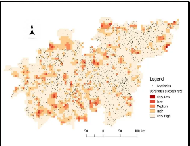
1- Borehole success rate (Figure 10):
The borehole success thematic map shows a big predominance of the light colour (5) meaning that the borehole success rate is mostly higher than 80% throughout all the region. There are also some spread smaller areas correspondent to lower percentages (darker colours) and even though they look well distributed a bigger incidence is
31 notorious in the western part of the map which makes sense considering the geology of the area.
Taking a deeper analysis of the current situation and considering the borehole´s distribution it is possible to identify some areas which are less represented, and this fact may have an influence on the produced maps. Most of the less represented areas are in the western side and, in this specific situation, correspond mostly to high borehole success rate percentages (>80%). It is possible that the presence of more boreholes in those areas could lead to significant changes in the map, making it darker. In an area with fissured porosity there are very high differences between the values from one place to another and therefore the more information available the more differences are likely to be spotted, showing more precisely where the fractures and weathering zones can be.
In the east side, a bigger quantity of boreholes is not expected to make such a big difference in the results, due to its geology.
2- Borehole yield (Figure 11):
32 Looking at the thematic map it is possible to understand how limited the extraction potential is all over the region, as the most used colour is the darker one equivalent to less than 5 m³/h.
The highest borehole yields are more likely to be found in thick sedimentary aquifers, particularly in poorly consolidated or unconsolidated sediments (MacDonald et al., 2012). Except from a small lighter area in the south-west part of Sikasso we can find most of the higher values (>20 m³/h) in the East, exactly where the sedimentary formations are known to be.
From the 2116 studied borehole locations there is a total of 1813 with information about the borehole yield and, from this total, 2 % correspond to values higher than 20 m³/h and 3 % inferior to 1 m³/h. This means that most of the places are capable of having a handpump to supply water for some of the basic community needs, although the places where groundwater can be abstracted at rates which are high enough for commercial irrigation are rare. It is very important to know where these rare areas are located. In case there is a need of big quantities of water extraction it is fundamental to focus on those areas and avoid overexploitation of the places that do not have enough water.
Comparing with the previous borehole success rate map, it is possible to see that the areas with higher borehole yields correspond to places where the borehole success is higher than 80%.
33 3- Borehole depth (Figure 12):
The drilling depth values are reasonably even in all the region (mostly between 50 and 100 meters). No boreholes were smaller than 25 meters and, out of 1893 locations,14 boreholes were longer than 150 meters, being 378 meters the highest registered value. All the areas with high values (>150 meters) were found in the east part of the study area.
In this case higher values correspond to lower groundwater potential scores as longer boreholes are needed to reach the water, also meaning more expensive drilling costs. Comparing the borehole depth map with the previous ones it is possible to realize that most of the areas with high success rates and borehole yields correspond to boreholes longer than 50 meters, except from one place in the east side where boreholes no longer than 50 are long enough to reach the groundwater. Considering it´s characteristics this area may have great potential for big commercial quantities of water extraction.
34 4- Electric conductivity (Figure 13):
In the electrical conductivity thematic map, the lighter colors, corresponding to the higher groundwater potential scores, correspond to lower values because the easiest the electrical current can pass through water (high values) the more particles are known to be present meaning an unsuitable drinking water for very high values. For the other values, this parameter does not give information about the quality of the water quality once it simply measures the ions dissolved. A medium value can, for example, be acceptable (even de desirable for some uses).
Looking at the map it is possible to realize that most of the area has values lower than 500 μS/cm (approximately 97%) meaning a most probable human consumption suitability all over.
The only exception found was an extremely high value of 5880 μS/cm inside Natien commune in a village called Tamba (Figure 14). Being the only extreme value found, it
35 can be either a local condition or even a typo in the database. It is also possible to distinct a northeast region where the values are higher than the average (with some medium and low values).
After the analyses of the produced thematic maps two other were created with the borehole success rate and borehole depth parameters. For that, new breaks were defined and are represented in Table 2 with Categories 2.
Using the previous breaks, the borehole success rate map ended up being colored mostly by the 5 (very high) correspondent light color, meaning a percentage higher than 80% almost all over. To be able to have a better distinction inside those 80% new breaks were defined, allowing to have a better perception of the areas where the values are higher than 90% and less than that. A bigger variation of the colors is represented in the map from Figure 15.
36
Figure 16-Borehole depth thematic map based on the new breaks. Figure 15-Borehole success rate thematic map based on the new breaks.
37 For the borehole depth, the same happened, and using the first breaks most of the area was colored with the 3 (medium) values, representing values between 50 and 100 meters. The new defined breaks separate that gap and it is possible to identify the boreholes with lengths between 50 and 75 meters as well as 75 to 100 meters. The map obtained was the one from Figure 16.
The thematic maps produced based on the new breaks are more representative to the specific Sikasso reality and allow a better understatement of the area. They are an important tool to have into consideration although they were not used to produce the final groundwater potential map.
After the creation and analyses of the four presented maps QGIS was also used to develop a groundwater potential one, based on a mathematical function responsible for adding the information of all the thematic maps. In the following figure this Sikasso map (and its borders) is available, together with the one produced on the previous work from all Mali (Figure 17).
In the first map (commune scale), from Figure 17, it is possible to notice a Sikasso division into two distinct zones. The groundwater potential is clearly generally higher in the east than in the west. It is also possible to conclude, that this difference corresponds to two distinct geological units, the Sedimentary Formations of the Cambrian/Precambrian and a domination of the Precambrian Basement respectively. In the second map (village scale), from Figure 17, it is also possible to identify this clear division but inside each area there is a lot more detail that can be very important to understand exactly where the water is. The lighter colours with bigger values correspond to better groundwater potential areas, whereas the darker colours correspond to worse groundwater potential ones.
While looking at the first map no lighter than the medium colour was found in the west part but looking at the second one some high and even very high valued areas can be spotted. Observing the east, it happens otherwise and while a big majority of the area is covered by high values in the first map, in the second map some smaller lower values are represented all over.
38 Also, by observing the second map, some bigger homogeneous areas, with less pixel’s differences, are easy to spot. They are more common in the west side and correspond exactly to the places with least boreholes´ information available, or even none, which is an indicator of the lack of credibility of the map in those specific areas. A bigger amount
Figure 17-Commune scale and village scale groundwater potential maps. Commune scale map adapted from (Díaz-Alcaíde et al 2017).
39 of information, or a better distribution of the boreholes would be needed in order to reduce these homogeneous colours and turn them into something more specific and closer to reality. The following map (Figure 18) emphasises the areas that should be a priority for the development of new boreholes.
After this analyses the produced groundwater potential final map was also compared to the geology of the region and for a better perception the geological map from figure 5 was put side by side with groundwater potential one (Figure 19).
The geological map presented in the Figure 19 was taken from a technical report on the Sikasso property (Sandy, 2017) and represents only the west side. Comparing the four specific correspondent selected regions in both maps it is possible to take several conclusions. In the areas 1 and 4 the groundwater potential map shows mostly high and very high values corresponding to the sedimentary rock formations and in the areas 2 and 3 the colors used are mostly darker, meaning medium to very low groundwater potential values, and correspond to areas where most of the rocks found are granites. In those same areas it is also possible to identify some smaller lighter regions that may correspond to fractures in those granites. These differences were expected to happen,
40 according to the geology of the region, but were not possible to see in the previous commune scale map.
The detached evidences help proving the credibility and coherence of the groundwater potential map produced and help identifying the most appropriate areas to extract groundwater from. In case there is the need of water extraction for commercial irrigation proposes the only place in this west side prepared to do so is the area 1 because it corresponds to the only place where the groundwater potential is very high, and the borehole yield is high enough to support such requirement.
A
B
Figure 19-A-Groundwater potential map and B- Geological map from the western part of Sikasso adapted from (Sandy, 2017).
41
6. Conclusions
One of the main purposes of this work was to produce a groundwater potential map in a southern region of Mali, called Sikasso, using some available spatially distributed borehole data, making it a contribution that provides additional support for groundwater management practices. QGIS was the software used to do so and the development of the final map was based in four different variables, the borehole success, yield, depth and electrical conductivity, which thematic maps were also produced. The same method has been previously used to create a groundwater potential map from all Mali (at a commune scale) and comparing both maps was another goal of this project that allowed a very important conclusion. It was possible to realise that this type of groundwater potential mapping at a smaller scale makes a big difference allowing the analyses of more detailed information.
In the commune scale map, it was only possible to identify one major geological difference separating Sikasso into higher groundwater potential values in the east and lower values in the west side. In the village scale map, it is still possible to identify that same difference but inside each side (east and west) more details are shown, and other conclusions can be taken.
In the west part of Sikasso the best and only possible area for commercial irrigation water extraction was clearly identified, as well as other areas with higher groundwater potential values. Some of them corresponding to sedimentary rocks ‘zones and some others to possible fractures in the granitic areas.
In the east part of Sikasso more areas with high groundwater potentials were found and, at this scale, it is also possible to identify those areas more clearly as well as the ones with lower values and less interest when it comes to the water exploitation.
The maps produced could be used to underpin water management practices although it was possible to conclude that there are some possible improvements to this work that could be done in the future to make it better and more complete, giving more and more precise information.
It would be useful to enhance the borehole database with new information, so it would be possible to estimate water access (something we cannot determine with the database
42 used). Other than that, it would also be important to make a better distribution of the boreholes, adding new ones to some specific places where they lack.
It would also be interesting to compare the results got in this work (at a village scale) with a groundwater potential map created at the same scale but using the indirect methods. Due to financial reasons it might not be possible to have such a good spatially distributed borehole´s data in some places and it would be interesting and important to understand whether the results obtained using a cheaper method would vary a lot from the ones obtained in this work.
Finally, the importance of groundwater in Mali cannot be underestimated and studying the country at this scale can be a very useful support to understand where the water is and plan how it should be used and where it should be taken from in the future. A good knowledge of the groundwater will prevent or reduce the impact of many negative impacts that might come from the population growth and lack of precipitation.
43
7. Bibliography
• AMIRA-International, 2013. P934A – West African Exploration Initiative – Stage 2. AMIRA International, Australia, Unpublished report.
• Balamurugan, G., Seshan, K. and Bera, S (2016). Frequency ratio model for groundwater potential mapping and its sustainable management in cold desert, India. Journal of King Saud University-Science.
• Ballo, I., Hein, K.A.A., Guindo, B., Sanogo, L., Ouologuem, Y., Daou, G., and Traore, A. 2016. The Syama and Tabakoroni goldfields, Mali. Ore Geology Reviews 78, 578–585.
• Diallo, D., and Diakité, D. 2011b. Permis de Sankarani – Rapport D’Activities Annuel 2011. Prepared for the Societe d’Exploitation et de Recherche Miniere. 32p.
• Diallo, M.M.A. 2011. Evolution du Climat. Direction Nationale de la Météorologie du Mali.
• Diallo, M., Diakité, D., Coulibaly, B., Doumbia, S., and Sangaré, S. 2016b. Permis de Kalé – Rapport Annuel 2016. Prepared for the Societe d’Exploitation et de Recherche Miniere. 18p.
• Diallo, M., Diakité, D., Coulibaly, B., Doumbia, S., and Sangaré, S. 2017b. Permis de Sankarani – Rapport Annuel 2016. Prepared for the Oklo Resources Ltd/ML Commodities. 18p.
• Diallo, M., Diakité, D., Coulibaly, B., Doumbia, S., and Sangaré, S. 2017c. Permis de Kourou – Rapport Annuel 2016. Prepared for REM. 17p.
• Díaz-Alcaide, S., Martinez-Santos, P., Martín-Loeches Garrido, M and Montero, E (August 2017). A survey of domestic wells and pit latrines in rural settlements of Mali: Implications of on-site sanitation on the quality of water supplies. Article in International Journal of Hygiene and Environmental Health.
• Direction Nationale de l’Hydraulique (2010). Données Hydrogeologiques et des Forages; Direction Nationale de l’Hydraulique; Ministère de l’Environnement, de l’Eau et de l’Assainissement: Bamako, Mali, 2010. (In French).
• EurGeol Dr. Sandy M. Archibald, PGeoAurum Exploration Services, August 31st, 2017. Technical Report on the Sikasso Property, Republic of Mali. Canada.
44 • Feybesse, J-L, Sidibé, Y.T., Konaté, C.K, Lacomme, A., Miehé, J.M., Lambert, A, Zammit, C, BRGM, CPG, DGGM. 2006b. Carte géologique de la République du Mali à 1/200 000, Feuille n° NC-30-XXII, Yanfolila. – Bamako (Mali): Ministère des Mines, de l’Énergie et de l’Eau.
• Ganapurm, S., Vijaya-Kumar, G.T., Murli-Krishna, I.V., Kahya, E. and Cüneyd Demirel, M (2008). Mapping of groundwater potential zones in the Musi basin using remote sensing data and GIS. Advances in Engineering software.
• Hussein, A.A., Govindu, V. and Medhin-Nigusse, A.G (2016). Evaluation of groundwater potential using geospatial techniques.
• Jenks GF (1967). The Data Model Concept in Statistical Mapping. International Yearbook of Cartography 7: 186–190.
• Jha, M. K., Chowdary, V. M., and Chowdhury, A., 2010. "Groundwater assessment in Salboni Block, West Bengal (India) using remote sensing, geographical information system and multi-criteria decision analysis techniques". Hydrogeology J.
• Jones, I., Earl, A., Bezuldenjout, G., van de Suy, S., Wild, G., and Coetzee, S. 2016. Avnel Gold Mining Limited (as Operator of SOMIKA) – Project Number J2227. NI 43-101 Technical Report on Kalana Main Project, Kalana,Mali. 342p. • Krishna-Gumma, M. and Pavelic, P (2012). Mapping of groundwater potential
zones across Ghana using remote sensing, geographic information systems, and spatial modeling.
• Kusnir I (1999). Gold in Mali. Acta Montanistica Slovaca. Rocnik 4 (1999) 4, 311-318.
• MacDonald AM, Bonsor HC, Ó Dochartaigh BÉ, Taylor RG (2012). Quantitative maps of groundwater resources in Africa. Environmental Research Letters, 7 (2), 024009. 10.1088/1748-9326/7/2/024009
• Martínez-Santos, P., Díaz-Alcaide, S and Villarroya, F. A Commune-Level Groundwater Potential Map for the Republic of Mali. Water 2017.
• Mitra, S. (2017). Mali´s Fertile Grounds for Policy Brief Conflict: Climate Change and Resource Stress. Planetary Security.
• Mondal, S (2011). Remote Sensing and GIS Based Ground Water Potential Mapping of Kangshabati Irrigation Command Area, West Bengal. J Geograp Natur Disast.
45 • Murray-Rust, H (2013). Climate change in Mali: Key issue in water resources
(USAID).
• Netherlands Commission for Environmental Assessment (NCEA), Dutch Sustainability Unit. (2015). Climate Change Profile: Mali.
• Olson, S.F., Diakite, K., Ott, L., Guindo, A., Ford, C.R.B., Winer, N., Hanssen, E., Lay, N., Bradley, R., and Pohl, D.1992. Regional Setting, Structure, and Descriptive Geology of the Middle Proterozoic Syama Gold Deposit, Mali, West Africa. Economic Geology 87(2): 310-331.
• Parra-Avila, L.A., Belousovab, E., Fiorentinia, M.L., Baratouxd, L, Davis, J. Miller, J., and McCuaig, T.C. 2016.Crustal evolution of the Paleoproterozoic Birimian terranes of the Baoulé-Mossi domain, southern West African Craton: U–Pb andHf-isotope studies of detrital zircons. Precambrian Research, 274, 25-60. • Rahmati, O., Samani, A.N., Mahdavi, M., Pourghasemi, H.R. and Zeinivand, H
(2015). Groundwater potential mapping at Kurdistan region of Iran using analytic hierarchy process and GIS. Arab Journal of Geosciences.
• Rapport national sur la mise en valeur des ressources en eau: Mali Une étude de cas du WWAP préparée pour le 2ème Rapport mondial des Nations Unies sur la mise en valeur des ressources en eau. L’eau, une responsabilité partagée. (2006) (in French).
• Sherbinin, A., Chain-Onn, T., Giannini, A., Jaiteh, M., Levy, M., Pistolesi., L. and Trzaska, S. (2014). Mali Climate Vulnerability Mapping. USAID.
• Sternberg, T. and Paillou, P (2015). Mapping potential shallow groundwater in the Gobi Desert using remote sensing: Lake Ulaan Nuur. Journal of Arid Environments 118 (2015) 21-27.
• Toure, A., Diekkrüger, B. and Mariko, A (2016). Impact of Climate Change in Groundwater Resources in the Klela Basin, Southern Mali. Article from the Hidrology.
• USGS (2012). A Climate Trend Analysis of Mali. Famine Early Warning Systems Network—Informing Climate Change Adaptation Series. Fact Sheet 2012–3105. US Geological Survey, 4p.
• World Wide Fund for Nature (Formerly World Wildlife Fund). (1986). Living Waters, Conserving the source of life.
46 • Yeh, H.F., Cheng, Y.S., Lin, H.I. and Lee, C.H (2016). Mapping groundwater recharge potential zone using a GIS approach in Hualian River, Taiwan. Sustainable Environment Research.
WEB
• CIA (Central Intelligence Agency), The World Factbook, 2011. Retrieved from https://www.cia.gov/library/publications/the-world-factbook/geos/ml.html.
• Climate normals. Climate Sikasso, Mali. (n.d.). Retrieved from http://en.allmetsat.com/climate/mali-burkina-faso.php?code=61297.
• Gis Resources. Types of interpolation methods. (n.d.). Retrieved from http://www.gisresources.com/types-interpolation-methods_3/.
• Mali Population. World population review. (2018-06-16). Retrieved 2018-09-01, from http://worldpopulationreview.com/countries/mali/.
• Mali, WaterAid Global. n.d. Retrieved from: https://www.wateraid.org/where-we-work/mali.
• Smedley P (2002). Groundwater quality: Mali. British Geological Survey and Water Aid, 5pp. Retrieved from http://nora.nerc.ac.uk/516317/. Last accessed: July 21, 2017.
• The Global Monsoon System. National Taiwan Normal University (NTNU). n.d. Retrieved from www.worldscientific.com by on 03/01/15.
• United Nations Office for Coordination of Humanitarian Affairs (OCHA), n.d. Retrieved from https://www.unocha.org/.
47
8. Appendix
•
An example of the database sheets provided by the “Direction Nationale de l´Hydraulique”, written in French (Fig. 20) and the information organized in the attribute table (Fig.21).48
49
•
Borders, with villages from Segou and Kolikouro, added to the initial Sikasso area (Fig. 22).Figure 22-Sikasso and study area (Sikasso + borders).
Some intermediate results were obtained during the maps production and some examples will be shown below.
•
Firstly, an example of a Grid data report made with Surfer 11. The following example corresponds to the grid information of the depth, using the kriging method.——————————
Gridding Report
——————————
Thu Jul 19 15:13:44 2018
Elapsed time for gridding: 1.06 seconds
50
Source Data File Name: C:\Users\Carolina\Desktop\TESE\QGIS\coordenadas xy\b_depth2.xls (sheet 'Qgis Attributes')
X Column: A Y Column: B Z Column: C
Data Counts
Active Data: 1892 Original Data: 1893 Excluded Data: 0 Deleted Duplicates: 1 Retained Duplicates: 1 Artificial Data: 0 Superseded Data: 0Exclusion Filtering
Exclusion Filter String: Not In Use
Duplicate Filtering
Duplicate Points to Keep: First
X Duplicate Tolerance: 5.3E-007 Y Duplicate Tolerance: 3.2E-007
Deleted Duplicates: 1 Retained Duplicates: 1 Artificial Data: 0 —————————————————————————————————————————— —— X Y Z ID Status —————————————————————————————————————————— —— -7.1691 11.4444 97 1449 Retained -7.1691 11.4444 49 1460 Deleted —————————————————————————————————————————— ——
Breakline Filtering
Breakline Filtering: Not In Use
Data Counts
51
Univariate Statistics
—————————————————————————————————————————— —— X Y Z —————————————————————————————————————————— —— Count: 1892 1892 1892 1%%-tile: -8.4333 10.3744 32 5%%-tile: -8.1289 10.597 40 10%%-tile: -7.8554 10.7713 43 25%%-tile: -7.2494 11.1494 50 50%%-tile: -6.3959 11.5851 60 75%%-tile: -5.7299 12.1479 73 90%%-tile: -5.1848 12.6024 86 95%%-tile: -4.8912 12.7508 100 99%%-tile: -4.5042 12.8906 140 Minimum: -8.7542 10.215 9 Maximum: -4.2303 12.966 500 Mean: -6.46742690275 11.6405692389 64.2066596195 Median: -6.3957 11.58545 60Geometric Mean: N/A 11.6220837798 61.1521462134 Harmonic Mean: N/A 11.6036440074 58.5354748916 Root Mean Square: 6.54191294414 11.6590745265 68.6015358342 Trim Mean (10%%): -6.46632924251 11.6383 62.0745742807 Interquartile Mean: -6.43147096093 11.6088402323 60.7064413939 Midrange: -6.49225 11.5905 254.5 Winsorized Mean: -6.47324112051 11.6437186575 62.05602537 TriMean: -6.442775 11.616875 60.75 Variance: 0.969526661079 0.431394619286 583.984239074 Standard Deviation: 0.984645449428 0.656806378841 24.1657658491 Interquartile Range: 1.5195 0.9985 23 Range: 4.5239 2.751 491 Mean Difference: 1.12991237189 0.754663867122 21.7336414953 Median Abs. Deviation: 0.74085 0.49665 11
Average Abs. Deviation: 0.82235935518 0.551461310782 14.7605708245 Quartile Dispersion: N/A 0.0428590437519 0.186991869919 Relative Mean Diff.: N/A 0.0648304951101 0.338495128451
Standard Error: 0.0226370229998 0.0150999947371 0.555571548777 Coef. of Variation: N/A 0.0564239055119 0.37637475602 Skewness: -0.0824012283609 0.117539949391 5.55747607028 Kurtosis: 2.20635899157 2.11029101028 77.5528779571 Sum: -12236.3717 22023.957 121479 Sum Absolute: 12236.3717 22023.957 121479 Sum Squares: 80971.2144407 257187.163598 8904075 Mean Square: 42.7966249687 135.934018815 4706.17071882 —————————————————————————————————————————— ——
Inter-Variable Covariance
52 ———————————————————————————————— X Y Z ———————————————————————————————— X: 0.96952666 0.29777688 3.0954003 Y: 0.29777688 0.43139462 0.56329589 Z: 3.0954003 0.56329589 583.98424 ————————————————————————————————
Inter-Variable Correlation
———————————————————————————————— X Y Z ———————————————————————————————— X: 1.000 0.460 0.130 Y: 0.460 1.000 0.035 Z: 0.130 0.035 1.000 ————————————————————————————————Inter-Variable Rank Correlation
———————————————————————————————— X Y Z ———————————————————————————————— X: 1.000 0.436 0.128 Y: 0.436 1.000 0.062 Z: 0.128 0.062 1.000 ————————————————————————————————
Principal Component Analysis
———————————————————————————————————————— PC1 PC2 PC3 ———————————————————————————————————————— X: 0.911872555374 0.911872555374 -0.410439095724 Y: 0.410440002377 0.410440002377 0.911887091428 Z: -0.00523900800441 -0.00523900800441 0.911887091428 Lambda: 584.001219788 1.08577395642 0.298166609767 ————————————————————————————————————————
Planar Regression: Z = AX+BY+C
Fitted Parameters ———————————————————————————————————————— A B C ———————————————————————————————————————— Parameter Value: 3.54272511096 -1.13966594275 100.385335627 Standard Error: 0.630477950843 0.945175420431 13.390143697 ———————————————————————————————————————— Inter-Parameter Correlations ———————————————————————————— A B C
53 ———————————————————————————— A: 1.000 -0.460 0.683 B: -0.460 1.000 -0.962 C: 0.683 -0.962 1.000 ———————————————————————————— ANOVA Table —————————————————————————————————————————— ——————————
Source df Sum of Squares Mean Square F —————————————————————————————————————————— —————————— Regression: 2 19523.0303168 9761.51515838 16.998204554 Residual: 1889 1084791.16577 574.267424972 Total: 1891 1104314.19609 —————————————————————————————————————————— ——————————
Coefficient of Multiple Determination (R^2): 0.0176788729022
Nearest Neighbor Statistics
————————————————————————————————— Separation |Delta Z| ————————————————————————————————— 1%%-tile: 0.00206155281281 0 5%%-tile: 0.00732461603089 1 10%%-tile: 0.0111606451426 3 25%%-tile: 0.0210237960416 6 50%%-tile: 0.0320655578464 12 75%%-tile: 0.0425010588103 23 90%%-tile: 0.0544210437239 38 95%%-tile: 0.0633378244022 53 99%%-tile: 0.0888709738891 100 Minimum: 9.99999999998e-005 0 Maximum: 0.210102189422 456 Mean: 0.0331612027642 18.6041226216 Median: 0.0320655578464 12
Geometric Mean: 0.0275014956219 N/A Harmonic Mean: 0.0152835255169 N/A
Root Mean Square: 0.0377355777303 32.5711369783 Trim Mean (10%%): 0.0321869911681 15.369348209 Interquartile Mean: 0.0318891059111 13.0337909187 Midrange: 0.105101094711 228 Winsorized Mean: 0.0321586881568 15.6210359408 TriMean: 0.0319139926362 13.25 Variance: 0.000324479958908 715.1435684 Standard Deviation: 0.0180133272581 26.7421683564 Interquartile Range: 0.0214772627687 17 Range: 0.210002189422 456 Mean Difference: 0.0193079983698 19.0556038786 Median Abs. Deviation: 0.0107517139029 7.5
Average Abs. Deviation: 0.0134290845501 12.6146934461 Quartile Dispersion: 0.338092276145 N/A
54
Relative Mean Diff.: 0.582246624381 1.02426780699
Standard Error: 0.000414126834875 0.614803105524 Coef. of Variation: 0.543204882713 1.4374323853 Skewness: 1.36989410317 8.66101448608 Kurtosis: 9.98645611592 122.289755757 Sum: 62.7409956298 35199 Sum Absolute: 62.7409956298 35199 Sum Squares: 2.69415848 2007183 Mean Square: 0.00142397382664 1060.87896406 —————————————————————————————————
Complete Spatial Randomness
Lambda: 152.025886762 Clark and Evans: 0.817747156102 Skellam: 2573.47854891
Gridding Rules
Gridding Method: Kriging Kriging Type: Point
Polynomial Drift Order: 0 Kriging std. deviation grid: no
Semi-Variogram Model
Component Type: Linear Anisotropy Angle: 0 Anisotropy Ratio: 1 Variogram Slope: 1
Search Parameters
Search Ellipse Radius #1: 2.65 Search Ellipse Radius #2: 2.65 Search Ellipse Angle: 0
Number of Search Sectors: 4 Maximum Data Per Sector: 16 Maximum Empty Sectors: 3
Minimum Data: 8 Maximum Data: 64
Output Grid
Grid File Name: C:\Users\Carolina\Desktop\TESE\QGIS\grelhas\b_depth2 kriging.grd
Grid Size: 61 rows x 100 columns Total Nodes: 6100
Filled Nodes: 6100 Blanked Nodes: 0
Blank Value: 1.70141E+038
55 X Minimum: -9 X Maximum: -4 X Spacing: 0.050505050505051 Y Minimum: 10 Y Maximum: 13 Y Spacing: 0.05
Univariate Grid Statistics
—————————————————————————————— Z —————————————————————————————— Count: 6100 1%%-tile: 20.2089666481 5%%-tile: 30.3537873089 10%%-tile: 37.245445496 25%%-tile: 47.447955921 50%%-tile: 56.4204467731 75%%-tile: 66.412184573 90%%-tile: 75.6096434595 95%%-tile: 83.7440089776 99%%-tile: 102.766055973 Minimum: 3.51495955514 Maximum: 363.441680951 Mean: 57.1344827243 Median: 56.4262425457 Geometric Mean: 54.5890585361 Harmonic Mean: 51.4593343591 Root Mean Square: 59.5835029344 Trim Mean (10%%): 56.6907311027 Interquartile Mean: 56.613081694 Midrange: 183.478320253 Winsorized Mean: 56.6393147788 TriMean: 56.6752585101 Variance: 285.891573229 Standard Deviation: 16.9083285167 Interquartile Range: 18.9642286521 Range: 359.926721396 Mean Difference: 17.8031678987 Median Abs. Deviation: 9.51742992463 Average Abs. Deviation: 12.2212464223 Quartile Dispersion: 0.166557221604 Relative Mean Diff.: 0.311601104093
Standard Error: 0.216488962816 Coef. of Variation: 0.295939119609 Skewness: 1.67248215666 Kurtosis: 24.0316177309 Sum: 348520.344618 Sum Absolute: 348520.344618 Sum Squares: 21656182.3138
56
Mean Square: 3550.19382193
——————————————————————————————