Anthropogenic influence on the degradation of an urban lake –
The Pampulha reservoir in Belo Horizonte, Minas Gerais, Brazil
Kurt Friese
a,n, Gerald Schmidt
b,c, Jorge Carvalho de Lena
d,
Herminio Arias Nalini Jr.
d, Dieter W. Zachmann
b,eaUFZ-Helmholtz Center for Environmental Research, Department Lake Research, Br¨uckstraße 3a, D-39114 Magdeburg, Germany
bInstitute for Environmental Geology, Technical University of Braunschweig, Germany
cDECHEMA e.V., Karl-Winnacker-Institut, Frankfurt/Main, Germany
dDepartment of Geology, EM, Federal University of Ouro Preto, Minas Gerais, Brazil
eInstitute of Ecological Chemistry and Waste Analysis, Technical University of Braunschweig, Germany
a r t i c l e
i n f o
Article history:
Received 29 September 2009 Accepted 2 December 2009
Dedicated to Prof. Dr. Walter Geller on the occasion of his 65th birthday anniversary
Keywords: Heavy metals Sediment Water anoxia Contamination Nutrient loading
a b s t r a c t
The artificial reservoir Lagoa da Pampulha in central Brazil has been increasingly affected by sediment deposition and pollution from urban and industrial sources. This study investigates water chemistry and heavy metal concentrations and their fractionation in the lake sediment using ICP-OES, ICP-MS, and XRD analyses. Fractionation analysis was done by sequential extraction under inert gas as well as after oxidation. The lake exhibits a permanent stratification with an oxygen-free hypolimnion below 2 m depth. Nutrient concentrations are enriched for phosphorous components (SRP, PO4). In the
sediment it was not possible to detect oxygen. Carbon, sulfur, and most of the analyzed heavy metals are enriched in the top sediment layer with a pronounced downward decrease, indicating the presence of an anthropogenic influence. Statistical analysis, including correlations and a Principal Component Analysis (PCA) of depth-related total concentration data, helps to distinguish presumably anthropogenic heavy metals from geogenic components. Some samples with high element concentrations in the sediment also show elevated concentrations in their pore water. Analyses of element distribution between sediment and pore water suggest a strong bonding of heavy metals to the anoxic sediment. The trend towards elevated solubility in the pore water of oxidized samples is clear for most of the analyzed elements. Fractionation analysis reveals characteristic associations of selected elements to specific mineral bonding forms. In addition, it indicates that the behavior of heavy metals in the sediment is strongly influenced by organic substances. These substances provide buffering against oxidation, acidification, and metal release. The high nutrient loading causes reducing conditions in the lake sediment. These conditions trigger the accumulation of sediments rich in S2, which stabilizes the fixation of heavy elements. In the future, care must be taken to reduce the supply of contaminants and to prevent the release of heavy metals from sediments dredged for remediation purposes.
&2009 Elsevier GmbH. All rights reserved.
Introduction
The influence of industrial activity on the environment is frequently expressed in an elevated influx of pollutants in surface waters. Heavy metals pose a special problem based on their strong tendency to accumulate and the impossibility to be eliminated chemically or biologically.
In lakes the sediment may be considered the ultimate destiny of heavy metals because solid substances accumulate with time and soluble forms in contact with water may become
solid material through precipitation, flocculation, adsorption, agglomeration, complexation, or by the assimilation in organic substances (e.g. intake by organisms), which is finally deposited
(Calmano, 1989; Salomons and F ¨orstner, 1984). Dissolution
of metals from sediments occurs less frequently under natural circumstances, but this effect cannot be excluded, if physico-chemical conditions change. The consequences on living organisms may be serious.
The urban environments are more susceptible to the influence of anthropogenic activities than their rural counterparts. They are characterized mainly by road networks, traffic, housing, energy generation plants, industry, and waste (Virkanen, 1998;
Charles-worth and Lees, 1999). Because of the variable intensity of these
activities, urban soil may range from undisturbed to man-made or
ARTICLE IN PRESS
Contents lists available atScienceDirect
journal homepage:www.elsevier.de/limno
Limnologica
0075-9511/$ - see front matter&2009 Elsevier GmbH. All rights reserved. doi:10.1016/j.limno.2009.12.001
n
Corresponding author: Tel.: +49 391 810 9200. E-mail address:kurt.friese@ufz.de (K. Friese).
ARTICLE IN PRESS
built-up (Kelly et al., 1996 and references therein), and this material represents the main source of chemical load to the bottom sediments of urban lakes (Virkanen, 1998). Of particular interest is the accumulation of metals in the water bodies of cities. Several studies have shown increase in metal content in aquatic environments as a consequence of urbanization (e.g.Lindstr ¨om, 2001) and contamination of urban soil (Kelly et al., 1996). Also the introduction of nutrients and particulate organics is of concern in urban areas. Given the intensity with which it occurs, it may lead to eutrophication and in some cases to ecologically irreversible deterioration of the lake.
The Pampulha Lake is located in the northern part of Belo Horizonte city, the capital of Minas Gerais state, Brazil. Belo Horizonte, with 2.5 million inhabitants, is the 4th-largest Brazilian city. A large part of the catchment area of this lake (97.91 km2) spreads over the surface of the neighbor city
Contagem. The reservoir itself possesses an area of 2.7 km2, a
total water volume of 12 million m3(max. depth 13.3 m) and it is
completely encompassed by a built city region.
The Pampulha dam was originally built up, in 1958, to store water and to prevent flooding in the region of the Pampulha stream. It was also planned as a reservoir of drinking water for the city of Belo Horizonte and as a recreation area for the population. The quickly growing population and industrialization of the area brought negative consequences which impaired the usage of the dam for its original purposes. The most obvious problem has been the silting up of the lake with an estimated input of 200,000– 400,000 m3of sediment per annum (Cena, 2001;CPRM, 2001), a
situation which got worse between 1994 and 1999 with a total income of 2 million m3/annum. Another problem is the detraction
of water quality. The eutrophication of the lake has been increasing since 1970 (Pinto Coelho, 1998), the availability of nutrients triggering such a high primary production that even with frequent withdrawal of biomass the dissolved oxygen is still being consumed. These nutrients are transported to the lake via eight small streams of which the most important and also the most polluted ones are Sarandi, Ressaca, and Agua Funda. Some measures have been adopted by local authorities to solve these problems. Among them are the ‘‘Programa de Recuperac-ao e~
Desenvolvimento Ambiental da Bacia da Pampulha em Belo Horizonte (Propam)‘‘ project (www.cmbh.mg.gov.br/index.
php?option=com_content&task=blogsection&id=44&Itemid=235;
Rose, 2001), for which so far an amount of US$ 150 million has
been spent.
The streams Sarandi and Ressaca provide together 70% of the total water income of the reservoir and their basin represents 63% of the total catchment area. A study ofRietzler et al. (2001) showed extremely high heavy metal pollution in these both streams. Potential sources for this contamination are iron and steel industries (Fe, Cr, Ni, Co), solvent and paint industries
(Ni, Cr, Pb), and the land-fill dump of Belo Horizonte (Fe, Mn, Ni, Cu, Cd, Pb, Zn). The outflow is controlled by an overfall spillway, and so the water level does not vary much throughout the year (Pinto Coelho, 1998). The water from the dam flows to the Pampulha stream, which in turn flows to the Velhas River.
The geological formation of the region is assigned to the Complexo Belo Horizonte (CPRM, 2001). It is composed of granite and gneiss with parts of migmatite. The age of gneiss and migmatite amounts to 2.8 Gyr. The granites are considered to be 2.7 Gyr old. Due to intensive weathering a large and deep soil covering has formed which is mainly composed of iron and aluminum oxides and shows a brown to red color. The soil has a sandy and a clayey texture with a poor cohesion. Therefore it is susceptible to erosion.
The climate of the region can be described as tropical mountain climate with dry winter and humid summer (K ¨oppen Cwa). The temperature shows little variation during the year with a mean maximum of 23.41C in February and a mean minimum of 18.51C in July. In contrast, the two seasons are quite clearly differentiated according to the mean precipitation values. The dry season (from April to September) shows a minimum of 13 mm in June, and the rainy season (from October to March) a maximum of 321 mm in December.
Some previous studies (Giani, 1994; Pinto Coelho, 1998) provide a good description of the lake. Its water shows strong signs of eutrophication and stratification and is very poor in oxygen. The quality of the water and its functionality are severely impaired. During our sampling work in August many dead fish were floating at the surface and no living ones could be seen.
The main goals of this work are to determine the dominant conditions in the water, the properties of the sediment, specifi-cally its mineralogical composition and particle size distribution, the kind and concentration of heavy metals in the sediment, and their origin, either anthropogenic or geogenic.
Material and methods
For this work two sampling campaigns were carried out to include effects of the two different climatic conditions, dry winter and humid summer. The first one took place at the end of the wet season on May 8, 9, and 15, 2001, and the second one at the end of the dry season on August 7, 8, and 9, 2001. The sample stations are shown in Fig. 1 and their UTM coordinates are A (23 K 606665 7804617), B (23 K 607019 7804528), and C (23 K 607960 7805109). All of them are located in the center between the two banks. Water data are available only for the first campaign.
Fig. 1.Sampling points in the Pampulha reservoir. Light gray areas=islands; black line=border of catchment area.
ARTICLE IN PRESS
For the water sampling new PET flasks were used. Analyses included physico-chemical parameters (T, O2, pH, Eh, and
electrical conductivity), main cations (Na+, K+, Ca2 +, and Mg2 +),
nutrients (NO3–N, NO2–N, NH4–N, N-total, SRP, and PO43), and
trace elements (Al, Fe, Mn, S, Si; As, Cd, Co, Cr, Cu, Pb, Sb, Sn, Zn). Samples were collected at each meter in depth ranging from the surface to the bottom. Physico-chemical parameters were determined in situ, using WTW instruments (WTW, Germany) and following the standard DIN specifications (DEV, 2001). The redox potential (Eh) was corrected for temperature. For the determination of trace heavy metals, samples were filtered with 0.45
m
m and preserved with nitric acid (pHo2) at 41C. For the determination of N species samples were also filtered and preserved with HgCl2; for the determination of P samples werepreserved with H2SO4. All the chemical analyses were conducted
according to the Standard Methods for the Examination of Water and Wastewater (Greenberg et al. 1992). The concentrations of main cations (Na+, Ca2 +, K+, and Mg2 +) and of trace elements (Al,
Fe, Mn, S, Si; As, Cd, Co, Cr, Cu, Pb, Sb, Sn, Zn) were determined using inductively coupled plasma spectrometry (ICP-OES). In all samples of surface and pore waters the concentrations of Al were below the detection limit (0.35 mg/L). The results were validated with the NIST 1643d reference material (
http://georem.mpch-mainz.gwdg.de).
At each sampling station and at each sampling campaign, up to six sediment cores were collected with a gravity corer, Mondsee-corer type from UWITEC Austria (Mudroch and Azcue, 1995). The samples were collected with water on top and brought to the shore undisturbed in Polycarbonate tubes (9 cm diameter, 1 m length). The water was allowed to flow out at the top by carefully pressing up the bottom of the tubes. The sediment was then cut into slices from top to bottom (0–1, 1–2, 2–3, 3–4, 4–5, 5–7.5, 7.5– 10, 10–12.5, 12.5–15, and 15–20 cm). The slices were homo-genized, packed into polyethylene bags or vessels, and kept refrigerated (o41C). At the second sampling campaign, one core from each sampling station was dedicated explicitly to analyses under unchanged physico-chemical conditions. While the materi-al from other cores was eventumateri-ally materi-allowed to dry at air, the material from these cores was always kept refrigerated in an Argon atmosphere to prevent oxidation. The corresponding samples are denoted ‘‘anoxic’’, the others ‘‘oxidized’’ in the results of the sequential extraction.
The sediment samples were dried in quartz evaporating dishes at 601C. Some samples were separated into their different grain size fractions for analyses of trace elements because the concentration of trace elements in sediments depends on the grain size (Salomons and F ¨orstner, 1984;Vester and Zachmann, 2003). These fractions were separated and their content of main and trace elements was determined. In this way specific differences in the enrichment in the various grain sizes may be found. In order to carry out the separation of the desired fractions, 7 g of the dry sediment was suspended in 150 mL of NH3
0.01 mol/L. To disaggregate the particles the suspension was left in an ultrasonic bath for 2 min (Bandelib Sonopuls HD 200, 200 W, 20 KHz, 130
m
m amplitude, 6 mm Ti plate, 60% power). The sand fraction was separated with a stainless steel sieve (63m
m). The remaining material was separated into different silt and clay fractions (20–63, 2–20,o2, and 52m
m) by flotation (Bachmannet al., 2001). The solid material of each grain size fraction was
separated by centrifugation, dried at 601C and finally weighed and kept in polystyrol vials.
Analysis of mineralogy and total elemental concentrations was carried out on the untreated samples, including all grain size fractions. Because of the correlation of elemental concen-trations with the grain size mentioned above, it is usually advisable to discard the sandy fraction (Salomons and F ¨orstner,
1984). However, in this case, this fraction was so small that it could be neglected; it was usually below 1% of the total dry weight.
The mineralogical identification followed the methodology described byZachmann (1994). The dry samples were ground in an agate mortar together with bi-distilled water to obtain a suspension. The suspension was applied to a glass plate (three plates per sample) and allowed to dry in a thin layer. One plate of each sample was then left in a desiccator filled with ethylene glycol for 24 h at 601C. Another sample plate was heated at 6001C for 1 h, and the third plate was analyzed with no further treatment. All determinations were carried out by X-ray diffrac-tion (Krischner, 1990) using a Philips PW 1730/10 instrument with a Cu tube (
l
=1.542 ˚A). The data evaluation was performed as described inZachmann (1994). In general, the obtained diagrams were interpreted manually on the basis of thePowder Diffraction Filedatabase (JCPDS, 1967; Hanawalt method). In addition, the evaluation used clay reference materials which were prepared in the geochemical lab of the Technical University of Braunschweig(Zachmann, 1994).
Pore water was extracted with a centrifuge (diameter 26 cm, 4000 rpm) and filtered through membrane syringe filters (pore size 0.2
m
m).For fractionation analysis on the bulk sediment, a six-step sequential extraction method was applied (Jakob et al., 1990;
Zachmann et al., 2009). This method is a variant of the 5-step
scheme developed by Tessier et al. (1979). The following fractions were obtained: (1) exchangeable (ammonium acetate), (2) carbonatic (sodium acetate), (3) easily reducible (hydroxyl ammonium chloride), (4) less easily reducible (ammonium oxalate + oxalic acid), (5) organic/sulfidic (hot hydrogen per-oxide, ammonium acetate), and (6) residual (HF digestion, see below).
For the main and trace element determination, about 200 mg of sample material was digested in open PTFE vessels with 7 mL of HNO3(65% v/v), 2 mL of HClO4(60% v/v), and 14 mL of HF (40% v/v).
The vessels were heated at 1401C for 7 h and at 1801C until dryness. The residue was dissolved in 20 mL HNO3(1.3 mol/L) for
24 h. The dilution factor resultant from the sample weighed mass and the amount of acid was used for the calculation of the concentration in the dry mass.
Elements were determined by ICP-OES (Bausch and Lomb ARL 3520 ICP Sequential Spectrometer and Fisons Instruments Maxim) and ICP-MS (Micromass Platform ICP). The analytical methods were verified by regular participation in quality control analyses using different certified reference materials (e.g. ring experi-ments).
All sediment data were submitted to Principal Component Analysis (PCA) (Backhaus et al., 1996). After a careful examination of the data, an outlier (Barium) and the As concentration of one core from each sampling point were excluded. The procedure was carried out on six different data sets: (1) all data; (2) data of 1st sampling campaign; (3) data of 2nd sampling campaign; (4) data of sampling station A (both seasons); (5) data of sampling station B (both seasons), and (6) data of sampling station C (both seasons). In order to minimize the large differences among the data, a normalization procedure was performed to obtain the normalized valuezkjaccording to the equation:
zkj¼
x0
kj
m
jsj
wherex0
kjis the lnxkj(the natural logarithm of the measured value
kfor the elementj),
m
jis the mean value of the logarithm of allmeasured data for the elementj, and
s
jthe standard deviation forthe logarithm of all measured data for the element j. These K. Friese et al. / Limnologica 40 (2010) 114–125
AR
TI
CL
E
IN
P
RE
S
S
Table 1
Physico-chemical parameters, nutrient, main and trace element concentrations in the water of the Pampulha reservoir for the first campaign (May 2001);T=Temperature, DO =dissolved oxygen; Eh =redox potential, EC=electric conductivity; (Al was below detection limit).
Station Depth (m)
T (1C)
DO (mg/ L)
pH Eh
(mV) EC (mS/ cm)
Na+ (mg/ L)
K+ (mg/ L)
Ca2 + (mg/ L)
Mg2 + (mg/ L)
S (mg/ L)
NO3– N (mg/L)
NO2– N (mg/ L)
NH4– N (mg/L)
Ntot (mg/ L)
Si (mg/ L)
SRP (mg/ L)
PO4 (mg/L)
Fe (mg/L)
Mn (mg/L)
Cr (mg/L)
Co (mg/ L)
Cu (mg/ L)
Zn (mg/ L)
As (mg/ L)
Cd (mg/L)
Sn (mg/L)
Sb (mg/L)
Pb (mg/ L)
A 0 24.9 5.70 7.60 420 291 23.0 8.25 26.7 2.74 1.62 0.41 33 3.6 5.1 6.4 6 220 0.23 0.02 1.14 0.79 12.4 n
1.10 0.22 0.04 0.27 2.34
1 24.0 2.69 7.42 390 293 23.9 8.18 25.5 2.59 1.97 0.05 27 3.8 4.8 6.4 7 321 o0.09 0.02 0.68 0.79 2.67 n 2.41 4.25 0.08 0.32 6.27
2 23.6 1.76 7.35 380 295 22.7 8.00 25.6 2.54 1.61 0.10 32 3.7 4.6 6.5 5 78 0.010 o0.01 1.04 0.61 0.83 n 0.97 0.13 0.02 0.58 1.18
3 23.5 0.56 7.36 400 298 25.9 8.15 26.3 2.59 2.53 0.12 35 3.8 5.0 6.3 6 407 o0.09 0.04 1.04 0.93 8.88 n 4.44 9.88 0.19 1.36 16.0
4 23.4 0.34 7.31 380 297 29.3 9.14 28.0 2.72 4.36 o0.05 13 3.8 4.8 6.7 3 947 0.22 0.16 1.83 1.42 23.8 n 6.67 16.1 0.30 0.83 36.5
5 23.3 0.30 7.30 370 298 22.6 7.72 25.1 2.48 1.56 o0.05 o6 3.9 5.0 6.5 6 171 o0.09 0.10 1.04 0.62 0.85 n 0.93 0.27 0.02 0.13 1.26
6 22.5 0.25 7.32 360 324 24.6 7.80 26.0 2.57 2.00 o0.05 13 4.2 5.5 6.5 8 283 o0.09 0.03 0.35 0.65 3.87 n 2.28 4.44 0.10 1.09 7.00
6.8 22.3 0.20 7.28 280 325 27.3 8.22 25.4 2.86 2.27 o0.05 o6 4.5 5.5 6.9 9 484 0.33 0.18 1.58 1.26 4.96 n 2.07 3.86 0.10 0.70 7.15
B 0 24.9 6.50 7.74 350 290 22.4 7.35 24.3 2.47 1.42 0.08 o6 3.1 6.2 6.5 470 131 0.12 0.03 0.94 0.73 1.24 18.1 1.07 0.17 0.08 0.20 0.94
1 23.8 2.56 7.51 360 298 23.6 7.65 24.7 2.57 1.78 0.17 o6 3.2 6.7 6.7 8 205 o0.09 o0.01 0.70 0.82 3.55 n 1.91 2.63 0.08 3.38 3.18
2 23.6 0.79 7.36 360 292 23.0 7.52 24.4 2.54 1.45 0.19 36 3.4 7.4 6.8 7 110 o0.09 o0.01 o0.03 0.65 1.65 28.4 0.95 0.12 0.03 0.36 0.71
3 23.7 0.34 7.32 350 291 22.8 7.46 24.7 2.53 1.54 0.28 10 3.6 8.5 6.8 20 57 o0.09 0.06 o0.03 0.58 0.61 5.2 0.85 0.07 o0.01 0.11 0.41
4 23.4 0.26 7.29 320 294 22.8 7.66 23.7 2.53 1.51 0.05 o6 3.4 5.6 6.5 480 151 o0.09 0.16 3.05 0.66 0.43 14.6 0.89 0.07 0.01 0.22 0.47
5 23.6 0.19 7.27 290 293 22.0 8.28 25.0 2.60 2.45 0.85 7 3.5 7.2 6.5 150 o28 0.29 0.22 0.51 0.82 1.33 18.6 1.06 0.13 0.04 0.23 2.41
6 23.4 0.28 7.25 320 293 22.1 7.75 24.8 2.46 1.41 1.03 15 5.4 16.2 6.9 60 241 0.36 0.27 0.61 0.75 1.03 9.1 1.01 0.08 o0.01 0.22 0.58
7 23.4 0.17 7.25 140 297 22.6 7.66 24.6 2.44 1.41 0.18 o6 5.0 8.5 6.6 530 621 1.03 0.42 0.07 0.85 17.1 14.4 1.20 0.07 0.06 0.25 0.96
8 23.0 0.22 7.12 80 322 23.6 7.87 24.6 2.49 1.55 0.48 9 6.0 10.9 5.0 490 497 0.60 0.30 0.38 0.81 0.94 15.8 1.04 0.08 0.06 0.15 2.29 9 22.8 0.20 6.99 90 328 22.4 7.51 24.1 2.42 1.32 0.82 o6 6.4 15.2 7.4 280 991 1.70 0.46 0.45 0.90 1.13 10.8 1.15 0.07 0.03 0.30 0.56
10 22.8 0.19 6.95 60 334 21.0 7.69 24.2 2.43 0.97 1.19 17 6.8 19.0 6.9 460 1334 3.23 0.65 0.87 1.13 0.56 5.9 1.50 0.11 0.08 0.22 0.40 11 22.6 0.28 6.80 40 358 13.1 6.88 23.2 2.23 0.35 0.32 15 12.1 nn
4.8 810 3416 9.37 1.30 1.18 1.56 0.50 9.4 2.10 0.09 0.08 0.78 0.61
C 0 22.8 0.55 6.85 130 307 21.5 7.75 25.2 2.58 1.19 o0.05 o6 4.6 6.6 6.8 60 150 1.14 0.50 0.28 0.83 0.75 4.5 1.11 0.06 0.03 0.14 0.51
1 22.9 0.44 6.97 120 307 20.9 7.56 23.9 2.43 1.18 0.05 7 4.8 7.0 6.8 60 65 1.01 0.49 0.30 0.84 0.75 4.5 1.12 0.06 0.04 0.15 0.52
2 22.6 0.28 6.96 110 310 20.8 7.52 24.6 2.37 1.13 o0.05 6 4.9 7.2 6.8 60 .65 1.01 0.50 0.31 0.95 1.59 6.9 1.18 0.09 0.06 0.15 0.86
3 22.5 0.28 6.99 100 311 20.8 7.21 24.4 2.40 1.14 o0.05 7 5.1 7.2 5.7 100 242 1.39 0.53 0.24 0.85 0.43 3.6 1.10 0.07 0.03 0.13 0.48
4 22.5 0.18 7.00 90 311 21.0 7.43 24.7 2.38 1.00 o0.05 6 5.3 7.1 6.7 170 714 1.86 0.56 0.32 0.86 3.17 8.5 1.16 0.07 0.07 0.25 0.72
5 22.4 0.23 7.00 90 310 21.1 7.47 25.0 2.39 1.00 o0.05 o6 5.3 7.5 6.8 180 658 1.81 0.54 0.87 0.80 0.52 4.8 1.12 0.05 0.05 0.16 0.63
6 22.6 0.18 6.99 90 310 20.9 7.57 24.8 2.40 1.05 o0.05 6 5.6 7.8 6.8 180 533 1.94 0.56 0.39 0.87 1.14 4.3 1.22 0.08 0.17 0.21 0.75
7 22.5 0.20 7.02 90 311 20.4 7.96 24.7 2.52 1.02 o0.05 o6 5.2 7.2 4.5 170 530 1.96 0.55 0.25 0.51 0.55 5.8 0.62 o0.01 o0.01 o0.01 0.47
8 22.6 0.18 7.00 80 310 20.1 7.58 23.9 2.41 0.96 0.05 o6 6.1 8.0 6.6 260 729 2.36 0.62 0.30 0.46 0.47 3.3 0.55 o0.01 o0.01 o0.01 0.33
9 22.5 0.18 6.97 80 315 19.1 7.04 24.0 2.34 0.61 o0.05 o6 7.1 9.6 6.8 440 1506 4.11 0.80 0.48 0.60 1.67 9.1 0.81 o0.01 0.03 o0.01 0.63
10 22.4 0.18 6.80 80 343 11.7 5.55 17.6 1.71 0.43 o0.05 o6 7.4 9.9 6.6 480 1059 3.10 0.61 0.31 0.47 2.03 5.9 0.57 o0.01 0.02 o0.01 0.45
11 22.2 0.16 6.72 80 347 18.5 7.11 23.7 2.31 0.39 o0.05 o6 8.9 11.3 6.8 630 2003 5.37 0.89 0.43 0.58 0.42 3.6 0.82 o0.01 0.02 o0.01 0.34
12 22.1 0.16 6.67 80 357 13.7 6.85 23.6 2.21 0.34 0.06 o6 8.5 10.3 6.7 740 2484 7.01 1.09 0.77 1.07 0.61 4.4 1.64 0.04 015 0.13 0.66
13.3 22.0 0.18 6.67 80 367 12.0 6.69 23.4 2.17 0.28 0.10 o6 10.8 13.4 6.4 970 3218 9.53 1.28 0.85 1.30 0.30 2.2 1.89 0.03 0.14 0.07 0.42
n
No reliable results. nn
Not determined.
K.
Friese
et
al.
/
Limnologica
40
(2010)
114
–125
ARTICLE IN PRESS
hydrochemical data were statistically analyzed with the SPSS software Student Version release 8.0.0 (SPSS Inc.).
Results and discussion
Water chemistry
Values for the physico-chemical parameters in water are presented inTable 1. The temperature decreases slightly from top to bottom. Values of Eh, O2, and electrical conductivity in the
water column show that there is no mixing of water in spite of this restricted variation of temperature. The pH remains around neutral. This shows the persistence of a situation which has already been registered in the literature (Giani, 1994;
Pinto Coelho, 1998). Table 1 shows the concentration of
nutrients, main components, and trace elements in the water obtained in the first campaign. Though the concentration of soluble reactive phosphorus (SRP) in some samples is below the limit of detection, high values preponderate in most samples (max. 970
m
g/L above ground at station C), confirming the other indicators for strong eutrophication of the lake. High concentrations of Mn and Fe at stations B (max. 1.3 mg/L for Mn and 9.37 mg/L for Fe) and C (max. 1.28 mg/L for Mn and 9.53 mg/L for Fe) are observed in the deepest water layers, 1–2 m above the bottom. Apparently the low redox potential (40–80 mV) is responsible for the dissolution of the oxides and hydroxides of these elements. Related to the dissolution of iron and manganese oxides and hydroxides, a re-liberation of arsenic and phosphorous species can be observed, which are known to adsorb strongly on these oxides/hydroxides. Correlated to increase in Fe, Mn, As, and P the EC increases remarkably below 8 m water depth at the stations B (from around 300 to 400m
S/cm) and C (from around 300 to 370m
S/cm).Compared with the concentration of some heavy metals in the rivers Sarandi and Ressaca measured byRietzler et al. (2001), the values measured in the lake water are diluted strongly, generally with decreasing concentrations from stations A to C (e.g. for Cr from max. 850
m
g/L in the river Sarandi to 1.14m
g/L in the surface water at station A, 0.94m
g/L at station B, and 0.28m
g/L at station C). Similar dilution effects are detected for Cu (380m
g/L to 12.4, 1.24, 0.75m
g/L), Cd (180m
g/L to 0.22, 0.17, 0.06m
g/L), and Pb (800m
g/L to 2.34, 0.94, 0.51m
g/L). For Fe and Mn this dilution effect is overcompensated by the upward diffusion of reduced Fe2 +and Mn2 + species leading to 1.14 and 0.56 mg/L for Fe and Mn, respectively, in the surface water at station C (compared to 0.23 and 0.02 mg/L for Fe and Mn, respectively at station A and 0.12 and 0.03 mg/L, respectively, at station B). According toRietzler et al. (2001) maximal values are 80 mg/L for Fe and
19 mg/L for Mn in the river Ressaca.
S is given as total sulfur (measured by ICP-OES), though it is essentially present as sulfate. This is important to be addressed because there is some sulfide precipitation taking place in the bottom of the reservoir, which must be the result of sulfate-reduction bacterial activity. The depth profiles of S at points B and C indicate an evident and progressive decrease towards the bottom. Because there are also much more reducing conditions in B and C than in point A (Eh values are 200 mV lower, seeTable 1), this may indicate that sulfate is being reduced by sulfate-reducing bacteria and precipitated as Fe and/or Cu sulfides (see chapter below).
Sediment mineralogy and geochemistry
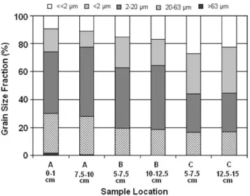
Fig. 2 shows the grain size distribution of the six sediment
samples which had been split up into grain size fractions. The
cores were without any visible structure and dark-gray to black in color. The sediment material was found to be very fine-grained, consisting of fine silt and clay. The clay fraction rises from roughly 25% at point A to over 50% at point C, while the silt fraction shows the opposite trend. Point B shows an intermediate composition. The main differences in grain sizes occur between the cores, not within the core. This fact was verified by using different depth intervals for the grain size analysis. The obvious reason for increase in clay content from station A to C is the increasing distance of the points from the main tributaries, which bring the main sediment load into the lake.
X-ray diffraction showed that the mineral composition of the sediment appears to be uniform throughout the whole reservoir. The main identified components are kaolinite (domi-nant), illite, and gibbsite. Goethite and hematite were also detected. A clear distinction can be made between minerals which are clearly detritic (allochtonous), such as the clay minerals kaolinite and illite, and those which could be partly the result of in situ precipitation (thus, autochtonous), such as Al (gibbsite) and/or Fe oxides (goethite, less likely hematite). A very rapid calculation of saturation indices for diverse minerals with some common geochemical modeling software (such as PHREEQC or MINTQA2) indicates that, at the surface, the water of the reservoir is clearly oversaturated with respect to several Fe phases such as ferrihydrite, goethite, or lepidocrocite. Therefore it might be possible that some of these phases could be precipitating.
Tables 2 and 3display the results from the chemical analysis of
the sediments for both campaigns. The depth profiles of selected element concentrations (Fig. 3) provide insights into the geo-chemical context of sedimentation. The dominant component, Al, shows an even distribution with a slight decrease in the top layer, where total carbon (TC) is more abundant than below. The distribution of S, Zn, and Cr concentrations consist of a strong enrichment in the top layer and almost constant values in lower depths. The same distribution is also found for TC, P, Mn, Cu, and Sb. A similar but less clear pattern is found for Fe, Pb, Ni, Sn, and Cd. The distinct enrichment in the upper layers of the depth profiles clearly indicates the presence of anthropogenic sources, whereas the deeper layers represent something close to the geogenic background. The mean concentration in the top 5 cm and the corresponding enrichment factors (divided by the minimum concentrations averaged from all sampling points) are
Fig. 2.Grain size distribution in the sediment samples of the Pampulha reservoir.
AR
TI
CL
E
IN
P
RE
S
S
Table 2
Physico-chemical parameters, dry mass (DM), main and trace element concentrations in sediments of the Pampulha reservoir (1st sampling campaign May 2001).
Station Depth (cm)
T (1C)
pH Eh
(mV) DM (%)
TC (mg/ g)
P (mg/ g)
S (mg/ g)
Al (mg/ g)
Ca (mg/ g)
Fe (mg/ g)
K (mg/ g)
Mg (mg/ g)
Mn (mg/ kg)
Na (mg/ kg)
Ti (mg/ g)
Ba (mg/ kg)
Co (mg/ kg)
Cr (mg/ kg)
Cu (mg/ kg)
Ni (mg/ kg)
Sr (mg/ kg)
V (mg/ kg)
Zn (mg/ kg)
Zr (mg/ kg)
As (mg/ kg)
Cd (mg/ kg)
Sn (mg/ kg)
Sb (mg/ kg)
Pb (mg/ kg)
A 0–1 23.6 6.75 30 20.3 34.3 1.47 2.18 144 4.27 42.4 11.9 2.23 433 1042 3.03 377 11.8 119 49.5 34.7 41.3 60.9 522 74.1 10.0 1.13 10.1 1.03 42.9 1–2 23.9 6.72 n
37.1 20.3 1.09 1.29 196 3.81 41.9 13.5 2.44 341 498 3.08 395 14.2 82.9 30.1 32.3 41.5 63.7 281 73.0 10.0 0.97 9.06 0.83 43.9 2–3 22.7 6.69 50 34.7 18.7 1.05 1.19 191 3.38 40.7 12.8 2.18 321 455 3.02 373 19.3 82.3 28.9 30.7 38.0 62.6 267 70.4 9.71 0.90 8.75 0.79 41.2 3–4 22.8 6.65 60 44.2 18.1 1.05 1.69 183 3.22 41.7 13.4 2.29 356 422 3.12 374 19.6 83.4 29.9 34.0 35.1 62.7 257 70.2 10.2 0.96 8.61 0.88 44.8 4–5 21.7 6.69 20 47.8 14.8 0.87 1.36 176 3.08 40.6 13.4 2.25 314 440 3.05 381 18.8 72.1 26.4 31.3 34.5 60.8 205 66.7 9.64 1.15 7.70 0.94 41.3
5–7.5 23.3 6.73 20 51.9 14.3 0.80 0.87 184 2.77 39.4 14.1 2.32 315 473 2.99 381 18.7 67.2 24.3 30.9 35.7 59.4 196 74.7 8.29 0.70 6.50 0.60 36.9
7.5–10 23.6 6.74 90 58.0 12.6 0.58 0.46 186 4.20 38.0 15.5 2.60 340 695 2.78 424 23.1 53.3 21.9 27.4 47.7 51.2 173 95.7 7.75 0.66 6.52 0.55 37.1 10–
12.5
23.4 6.85 n
58.8 15.5 0.64 0.46 172 4.51 33.3 15.1 2.62 368 595 2.75 423 25.2 57.5 24.1 28.7 48.1 50.9 199 90.7 8.38 0.74 7.11 0.60 38.9
12.5– 15
23.2 6.78 10 49.4 16.3 0.84 0.84 179 4.30 39.6 14.6 2.64 361 528 2.84 404 20.1 63.7 25.1 31.6 44.6 55.6 224 77.0 8.55 0.77 7.21 0.70 38.5
15–20 22.8 6.68 10 48.0 24.9 1.35 1.20 186 5.81 42.2 13.9 2.53 419 530 2.85 413 18.9 83.8 32.4 36.1 51.7 56.8 355 74.8 8.83 0.86 8.42 0.87 40.7 B 0–1 24.1 6.63 20 19.8 30.2 1.59 3.60 187 1.50 42.9 11.1 1.66 375 296 3.14 354 17.7 99.1 33.2 38.6 27.2 68.4 341 63.9 10.7 0.82 7.65 0.87 39.8 1–2 23.8 6.60 80 6.5 72.3 2.72 7.05 153 2.76 43.0 10.5 1.74 709 360 2.88 396 15.8 132 55.8 42.3 33.8 64.0 564 59.3 5.68 0.47 4.22 0.59 21.7 2–3 23.2 6.50 160 23.4 24.1 1.44 4.14 188 1.63 44.1 11.9 1.76 426 322 3.27 362 15.5 88.0 30.3 39.0 28.9 66.7 250 65.0 10.7 0.81 7.11 0.82 39.6 3–4 22.4 6.50 70 25.6 18.7 1.25 3.89 190 1.98 45.4 10.8 1.60 331 266 3.61 283 16.3 82.7 28.3 40.0 25.9 67.2 201 61.2 9.83 0.75 6.77 0.78 38.8 4–5 23.0 6.55 50 31.2 15.0 1.10 1.91 2030 1.03 43.3 10.5 1.49 293 246 3.73 269 16.8 68.7 24.9 35.8 23.5 67.9 180 62.8 11.1 0.71 6.49 0.72 39.1 5–7.5 22.7 6.55 50 38.8 15.5 1.08 1.40 188 2.86 35.6 14.8 2.05 308 432 3.19 394 17.1 64.9 24.2 33.0 32.1 56.5 208 63.2 8.92 0.73 6.73 0.69 37.0 7.5–10 23.7 6.53 50 24.6 31.2 2.43 4.80 172 2.60 50.0 10.7 1.59 551 330 3.18 345 20.0 92.3 32.1 47.3 30.6 62.3 325 57.4 7.65 0.60 5.37 0.72 28.5 10–
12.5
23.1 6.64 60 45.7 11.4 0.85 1.15 199 0.88 35.5 14.1 1.79 232 357 3.22 355 17.4 57.2 21.6 32.0 24.4 59.1 149 61.4 9.62 0.68 6.18 0.68 36.0
12.5– 15
22.8 6.55 50 40.1 16.8 1.11 1.96 180 1.02 35.7 13.3 1.95 229 337 3.25 357 19.4 67.5 25.1 35.4 26.0 60.8 171 55.0 10.0 0.73 6.68 0.77 36.9
15–20 23.4 6.58 20 37.4 22.7 1.54 2.27 175 1.24 33.8 13.7 1.87 281 329 3.00 309 16.2 89.0 27.2 41.3 26.2 55.7 297 56.1 6.72 0.57 5.19 0.60 28.9 C 0–1 6.66 50 14.7 32.7 1.74 5.72 173 6.60 47.6 9.07 1.56 364 269 3.66 271 20.8 81.9 30.2 43.1 38.7 77.2 246 59.9 11.5 0.85 7.36 1.01 41.0 1–2 6.58 50 14.5 47.8 2.42 7.94 182 7.71 52.5 8.98 1.66 582 260 3.45 278 20.0 88.3 32.8 53.0 44.5 75.0 310 59.6 13.0 0.93 7.71 1.33 41.4 2–3 6.59 50 16.7 46.2 2.41 7.81 180 6.55 51.1 8.43 1.44 537 248 3.33 266 20.2 85.5 33.3 54.0 41.0 74.2 299 61.3 12.7 0.95 7.47 1.31 42.0 3–4 6.56 50 11.8 59.0 3.95 12.3 160 5.60 59.0 6.72 1.31 1013 244 3.02 237 22.1 117 55.5 70.6 37.2 73.2 473 60.1 14.0 1.13 8.26 1.76 44.9 4–5 6.50 60 14.5 38.1 2.20 9.21 175 3.00 49.6 7.26 1.24 515 241 3.22 236 23.2 96.5 34.2 54.2 27.4 75.4 321 65.4 13.3 1.01 7.69 1.52 44.4 5–7.5 6.64 30 25.6 26.2 1.35 6.15 170 1.56 46.5 8.05 1.23 272 216 3.39 230 21.3 86.3 32.7 51.9 23.6 78.2 256 66.1 10.5 0.95 8.17 1.37 44.4 7.5–10 6.51 60 24.1 29.0 1.44 6.19 206 1.97 49.7 7.83 1.34 277 201 3.72 218 21.4 96.7 34.7 51.3 24.2 79.6 317 65.6 10.3 1.13 8.68 1.28 48.1 10–
12.5
6.65 40 25.5 23.1 1.50 5.42 205 3.02 46.0 7.41 1.31 259 199 3.62 220 20.3 92.4 32.4 49.7 27.2 81.9 277 68.2 11.0 1.04 8.63 1.05 46.8
12.5– 15
6.60 50 29.5 22.6 1.33 5.64 204 2.50 46.7 7.07 1.18 251 202 3.64 213 17.9 90.0 31.3 54.9 25.1 81.6 239 64.8 11.2 1.09 8.77 1.02 45.1
15–20 6.58 50 32.8 18.6 1.29 4.31 186 1.14 43.2 7.34 1.12 218 205 3.64 203 21.5 76.2 27.7 45.9 19.8 81.9 183 65.4 10.1 0.92 8.21 0.81 43.1
n
Not reliable values.
K.
Friese
et
al.
/
Limnologica
40
(2010)
114
–125
AR
TI
CL
E
IN
P
RE
S
S
Table 3
Physico-chemical parameters, dry mass (DM), main and trace element concentrations in sediments of the Pampulha reservoir (2nd sampling campaign August 2001).
Station Depth (cm)
T (1C)
pH Eh
(mV) DM (%)
TC (mg/ kg)
P (mg/ kg)
S (mg/ kg)
Al (mg/ kg)
Ca (mg/ kg)
Fe (mg/ kg)
K (mg/ kg)
Mg (mg/ kg)
Mn (mg/ kg)
Na (mg/ kg)
Ti (mg/ kg)
Ba (mg/ kg)
Co (mg/ kg)
Cr (mg/ kg)
Cu (mg/ kg)
Ni (mg/ kg)
Sr (mg/ kg)
V (mg/ kg)
Zn (mg/ kg)
Zr (mg/ kg)
As (mg/ kg)
Cd (mg/ kg)
Sn (mg/ kg)
Sb (mg/ kg)
Pb (mg/ kg)
A 0–1 6.67 70 11.3 85.8 5.60 3.88 129 6.10 52.6 11.7 2.44 1177 1038 3.54 504 17.1 210 71.0 43.6 61.3 60.4 1252 81.9 8.89 1.47 12.6 1.38 46.8 1–2 6.70 80 23.2 40.1 2.68 2.21 161 4.67 50.2 14.6 2.61 543 930 4.26 468 12.1 133 43.8 37.1 48.1 63.7 631 71.3 8.86 1.17 10.4 1.13 44.9 2–3 6.70 70 34.3 24.2 1.35 1.25 163 3.48 44.4 15.2 2.50 260 906 4.33 421 15.7 105 35.8 37.9 41.1 69.1 432 76.2 8.89 0.97 8.71 0.88 41.9 3–4 6.73 70 43.1 18.8 1.04 0.71 166 3.14 42.5 15.8 2.62 202 950 4.30 433 13.1 7606 27.7 33.0 40.7 66.9 256 77.7 8.19 0.82 7.30 0.70 39.2 4–5 6.73 40 42.0 20.4 1.09 0.86 155 3.08 40.2 15.2 2.46 211 880 4.00 438 14.8 80.9 313.3 34.4 42.2 66.4 273 74.6 8.05 0.82 7.61 0.73 40.0 5–7.5 6.77 50 45.6 19.0 0.94 0.66 155 4.18 41.9 16.0 2.76 228 1047 4.006 457 16.0 78.4 31.6 35.0 48.6 65.4 246 82.2 5.36 0.50 4.85 0.45 26.5 7.5–10 6.80 60 46.3 15.0 0.83 0.67 166 2.80 43.4 16.5 2.52 218 1035 4.31 442 13.4 67.6 24.0 31.7 39.6 63.1 205 85.6 5.76 0.52 4.66 0.42 28.3 10–
12.5
6.81 80 51.6 14.5 0.66 0.45 159 3.72 40.2 17.6 2.80 237 1566 3.87 487 12.8 58.0 24.1 28.9 51.0 56.6 185 106 7.84 0.73 6.59 0.59 38.2
12.5– 15
6.84 60 49.0 15.8 0.78 0.54 158 4.17 41.0 17.0 2.71 246 1330 3.90 481 15.1 64.2 26.2 32.3 52.1 59.8 219 105 7.63 0.73 6.55 0.61 37.6
15–20 6.87 40 47.6 18.7 0.89 0.61 161 3.96 42.7 16.7 2.71 245 1117 4.09 469 17.4 73.1 29.6 33.5 48.6 63.4 254 82.7 8.56 0.86 7.63 0.81 40.7 B 0–1 21.0 6.86 80 2.44 14.1 12.3 21.5 123 7.09 89.2 9.95 1.99 1878 1656 3.41 720 24.6 224 65.3 66.0 71.9 66.7 1292 493.7 11.6 1.60 11.6 2.49 46.3 1–2 20.1 6.81 60 14.4 58.9 2.97 5.00 154 2.59 54.6 10.7 1.76 542 524 4.27 464 18.9 144 48.6 43.6 35.7 73.0 662 65.3 10.9 1.26 10.0 1.54 47.3 2–3 19.8 6.80 70 23.5 26.5 1.64 2.63 168 1.77 47.8 12.1 1.82 289 527 4.46 407 17.0 101 35.1 38.8 30.6 74.4 311 62.9 10.1 0.91 7.87 0.93 42.7 3–4 19.8 6.80 70 28.2 20.5 1.40 1.95 178 1.69 49.4 12.1 1.75 220 415 5.00 378 19.5 85.4 29.2 38.4 27.8 74.8 222 63.1 10.0 0.89 7.11 0.90 41.1 4–5 19.9 6.83 70 38.9 14.7 1.19 0.74 165 1.41 40.3 15.3 2.31 199 747 4.30 429 14.7 65.0 24.9 33.0 26.7 66.6 187 62.5 8.84 0.78 6.69 0.66 38.7 5–7.5 20.2 6.83 50 24.4 41.2 2.91 3.69 152 4.06 49.2 12.1 1.85 456 568 3.87 403 14.7 105 37.6 51.0 37.4 68.8 395 60.9 11.3 1.08 8.59 1.18 43.2 7.5–10 20.8 6.82 40 35.2 15.2 1.02 1.05 179 1.11 43.2 14.9 2.17 165 683 4.46 407 18.3 68.2 26.2 37.7 27.5 68.7 175 63.8 10.4 0.83 6.89 0.75 42.0 10–
12.5
20.5 6.85 80 40.8 13.7 0.88 0.85 168 1.14 39.8 14.4 2.06 150 574 4.20 400 16.0 64.7 23.3 35.3 27.9 66.7 160 63.6 7.49 0.65 5.15 1.44 31.3
12.5– 15
20.7 6.83 60 47.9 17.3 0.72 0.49 162 2.89 41.5 16.4 2.70 327 749 3.93 437 17.3 62.9 25.0 33.1 35.9 62.6 194 62.8 9.29 0.84 7.27 0.68 40.1
15–20 21.3 6.85 30 33.6 26.9 1.83 2.77 159 2.38 41.7 14.6 2.29 251 627 3.76 413 17.1 110 32.7 50.0 35.1 61.4 394 61.2 9.24 1.00 7.91 1.00 41.6 C 0–1 19.7 6.80 90 12.8 46.5 2.05 8.13 185 3.50 62.4 8.46 1.63 383 519 4.81 303 20.8 102 35.1 51.0 35.2 73.4 382 58.9 14.0 1.18 8.79 1.37 46.2 1–2 20.4 6.78 90 17.4 32.6 1.76 5.28 194 3.72 58.0 9.87 1.80 365 556 5.09 319 20.9 84.4 28.7 41.1 36.2 73.5 254 61.9 13.6 0.99 7.66 1.09 44.8 2–3 19.0 6.84 90 17.4 45.1 2.00 6.26 192 6.50 61.4 10.6 1.88 406 614 4.99 361 19.2 81.0 28.7 47.2 47.7 69.3 276 64.3 12.8 0.96 7.01 1.21 41.1 3–4 19.1 6.87 40 16.3 49.7 2.29 7.17 181 7.17 61.4 10.4 1.87 533 615 4.59 373 19.9 84.2 32.1 52.5 52.5 70.1 311 59.8 14.0 1.04 7.41 1.38 44.1 4–5 19.1 6.85 60 18.1 37.5 2.00 6.74 193 3.98 59.4 9.71 1.77 412 571 4.81 314 17.5 82.7 30.7 46.7 38.8 72.2 279 65.2 14.3 1.08 7.57 1.35 46.3 5–7.5 20.0 6.78 70 17.8 37.4 2.33 7.18 194 2.04 60.3 10.2 1.77 401 569 4.88 300 21.6 95.8 33.1 56.8 30.5 72.6 320 64.9 14.5 1.18 8.10 1.52 47.7 7.5–10 19.8 6.77 60 19.6 25.6 1.42 6.75 161 2.58 45.3 8.97 1.71 246 454 4.29 289 19.9 82.8 31.0 51.3 27.4 72.2 239 64.5 13.6 1.08 7.79 1.44 48.7 10–
12.5
20.4 6.80 80 18.2 28.2 1.51 8.07 159 2.67 48.0 7.82 1.57 228 399 4.17 281 18.0 100 36.7 58.9 30.7 74.4 371 66.2 9.08 0.75 5.76 0.89 32.6
12.5– 15
20.3 6.80 40 22.4 26.6 1.54 4.98 173 6.18 48.2 8.08 1.62 232 371 4.61 272 23.0 94.8 32.4 55.1 34.8 77.1 303 66.6 14.1 1.11 8.70 1.14 47.3
15–20 20.9 6.83 60
nNo reliable values.
K.
Friese
et
al.
/
Limnologica
40
(2010)
114
–125
ARTICLE IN PRESS
listed inTable 4. The concentrations of C, S, and P are a clear indication of organic pollution as a consequence of urban wastewater discharge. Previous studies have shown that the reservoir is a sink for large amounts of nutrients introduced from the tributaries (Barbosa et al., 1998). The high sulfur contents are especially evident in the top sediment layer through a strong H2S
smell and black color.
Another point of interest that should be addressed here is the possible nature of the sulfides which seem to be forming near the sediment top layer. Some preliminary PHREEQC calculations using the data ofTable 3offer no possibility for the formation of pyrite or any other FeS phase; it allows, however, the possible formation of an amorphous CuS. But if only some HS or H
2S is allowed to exist in
the system (in the order of
m
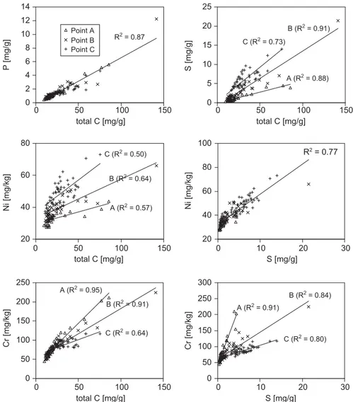
g/L), the water becomes saturated with respect to most common Fe and Cu sulfides.Two-element correlations (Fig. 4) reveal some more striking differences between specific elements. C and P show a clear unique correlation with no differences between the sampling points. C and S, in contrast, are correlated differently for each sampling point. Obviously, organic substances in the sediment have higher S contents at point C than at point A, with point B possessing intermediate amounts. The same is true for the correlation of C and Ni, indicating that Ni is uniquely correlated with S (Fig. 4). Cr shows a different behavior. Plotted against C, the steepest correlation line is found at point A and the flattest one at point C. This trend is even more pronounced in the correlation against S. Zn and Cu display the same pattern as Cr (not shown here). The different correlation patterns indicate that S is deposited not only in organic material with C and P, but also occurs as sulfide mineralization of Cu and Zn, more notably in the deeper water regions at sampling point C. This
observation is in close agreement with the lack of oxygen and the low redox potential at this station as well as with decrease in S in the deep water. The correlations also reflect the supply of heavy metals to the lake sediments by the main tributaries, the Sarandi and the Ressaca (Fig. 1). Ni is obviously closely linked to S, whereas Zn, Cr, and Cu seem more related to C, with a tendency to precipitate closer to the main tributaries than S and Ni. None of these elements shows any clear correlation to Fe or Mn concentrations.
A principal component analysis (PCA,Table 5) was done as a statistical summary of all the analyzed total concentrations
(Boruvka et al., 2005). The results vary somewhat depending
on the data set for which the PCA was calculated. In all cases three principal components were found to be of significance. Factor loadings 40.6 or o0.6 are printed in bold letters, since they are taken as an indication that the specific element can be assigned to the corresponding component. The following observations can be made:
Component 1 predominates by the very high communalities and factor loadings. The third component is obviously less significant. The elements C, S, Fe, Cr, Ni, and Sb are unambiguously assigned to component 1, irrespective of the data set used for the PCA. The factor loadings are positive in all cases. The elements P, Cd, Cu, Sn, and Zn are also assigned to component 1 with positive factor loadings in most cases. Depending on the data set, other elevated positive factor loadings occur. This applies especially to the data set from the first sampling campaign.0
10
20
30
40 0
TC [mg/g]
0
10
20
30
40 0
P [mg/g]
0
10
20
30
40 0
Al [mg/g]
depth (cm)
0
10
20
30
40 0
S [mg/g]
0
10
20
30
40 0
Zn [mg/kg]
0
10
20
30
40 0
Cr [mg/kg]
100 200 300 50 100 500 1000 1500
2 4 6 2 4 6 100 200 300
Fig. 3.Depth profiles of selected element concentrations in three different sediment cores from sampling point A (2nd sampling campaign August 2001).
Table 4
Mean concentration c [mg/kg] in top layer (5 cm) and relative enrichment factors EF (by dividing by the minimum concentration averaged from all sampling points) of selected elements in the sediment.
Element S P TC Zn Sb Cd Cu Cr Sn Pb Ni
c 4780 2170 37,640 383 1.07 1.09 36.8 102 8.0 43.5 42.6
EF 11 4.1 3.5 3.1 2.5 2.4 2.1 2.0 1.9 1.8 1.4
ARTICLE IN PRESS
The allocation of Mn and Pb to component 1 is even more ambiguous. While it is valid in most cases, also with positive factor loadings, there are some elevated positive or negative correlations to other components too, depending on the data set. An influence of the sampling point cannot be detected. The elements Al, K, Mg, Na, and Ba show either high positivefactor loadings in component 2 or negative ones in component 1. The only exception is a high positive factor loading for Ba in the data set of point B.
The elements Ca, Ti, As, Co, Sr, V, and Zr cannot be allocated to any component.Comparing these results with the depth profiles (Fig. 3) reveals that the elements assigned to component 1 are mainly the ones that show enrichment in the top sediment layers. Some of the clear correlations among these elements have already been presented above. The elements are typical components one would expect from pollution sources. According toRietzler et al.
(2001)the main pollution sources are iron and steel industries,
which probably are responsible for Fe, Cr, and Ni contamination and the land-fill dump of Belo Horizonte which might be the source for organic pollution. The concentration values of elements within the 2nd component show trends which are contrary to those of component 1. This is most evident in the depth profiles of Al and K, which are less concentrated in the top
layers. The assumption can be made that the elements within component 2 represent the components of the unpolluted sediment material, which is basically the soil eroded within the catchment. This interpretation fits well with the intensive weathering of the granitic sources in the catchment yielding a large and deep soil cover consisting mainly of easily eroded iron and aluminum oxides.
Pore water and fractionation analysis
Some samples with exceptionally high elemental concentra-tions in the sediment also show high elemental concentraconcentra-tions in the pore water. Zn is the most easily soluble of the trace elements, reaching up to4100
m
g/L, followed by Ni with up to 20m
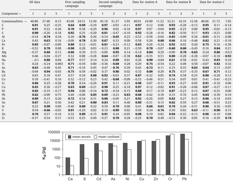
g/L.For estimation about the behavior of the elements in case of a remediation measure of the lake which will bring oxygen down to the bottom of the lake, selected samples were measured originally and after oxidation in the lab. Differences of elemental concen-trations in pore water between originally anoxic and oxidized samples are summarized inFig. 5. The distribution coefficientKd
is calculated by dividing the mean concentration in the sediment by the mean concentration in the corresponding pore water samples. Most elements become more soluble (lower Kd) after
oxidation; exceptions are Zn, Cu, and Cr. S shows the most significant difference, as can be expected from the conversion of
A (R2 = 0.88) B (R2 = 0.91)
C (R2 = 0.73)
0 5 10 15 20 25
0
total C [mg/g]
S [mg/g]
A (R2 = 0.91)
B (R2 = 0.84)
C (R2 = 0.80)
0 50 100 150 200 250 300
0
S [mg/g]
Cr [mg/kg]
A (R2 = 0.95)
B (R2 = 0.91)
C (R2 = 0.64)
0 50 100 150 200 250
0
total C [mg/g]
Cr [mg/kg]
R2 = 0.87
0 2 4 6 8 10 12 14
0
total C [mg/g]
P [mg/g]
Point A Point B Point C
A (R2 = 0.57) B (R2 = 0.64)
C (R2 = 0.50)
20 40 60 80
0
total C [mg/g]
Ni [mg/kg]
R2 = 0.77
20 40 60 80 100
0
S [mg/g]
Ni [mg/kg]
50 100 150
50 100 150
50 100 150 10 20 30
10 20 30 50 100 150
Fig. 4.Correlations of selected pairs of total element concentrations in sediment samples from the three sampling points.
ARTICLE IN PRESS
sulfide to sulfate. The pH in the pore water of most samples was found to decrease from 7 to values between 4 and 5 within 60 days of air exposure, which can be mainly attributed to sulfide oxidation.
The pH of the sediment is in the range of 7. In contrast to the pore water, the sediment samples show no change in pH even after several weeks of oxidation. The logical conclusion is that the sediment provides strong Eh and pH buffering. This observation is in good agreement with the high mass concentration of carbon (Tables 2 and 3) in the uppermost part of the sediment (0–5 cm) at all three stations (around 35–70 mg/g; highest enrichment factor 3.5, seeTable 4) which probably act as organic or inorganic carbon buffer against acidification.
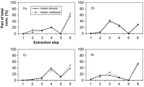
The elemental concentrations in the sequential extraction fractions are shown in relation to the total concentrations.Fig. 6 displays the averaged results from six well-preserved (anoxic) and four oxidized samples for the elements Fe, Zn, Cr, and Ni.
With Fe we observe a remarkably high share of the residual fraction, which increases in the oxidized samples. Increase in this
share is attributed to an increased presence of highly crystalline Fe oxide phases. Zn is mainly found in the 3rd, 4th, and 6th extraction steps. Zn found in steps 3 and 4 is bound to Fe oxides. It is not detectable in step 5, which was unexpected because the close correlations between the total concentrations of C, S, and Zn. These findings suggest a dominating organic speciation. Since the chemicals used for step 5 in the sequential extraction scheme are not appropriate for all kinds of sulfides (hypogene sulfide minerals like pyrite, chalcopyrite, or molybdenite might partly survive this leach) the residual fraction might contain some sulfidic residue not extracted in the 5th step. Zn fractionation shows no differences between anoxic and oxidized samples. Cr dominates in the 4th and 6th extraction steps, with a slight increase in the residual fraction for the oxidized samples. This is in good agreement with the well-known association of Cr and Fe oxides. Ni is partly soluble in the first four extraction steps, but the major part remains insoluble (residual phase). Part of the carbonate fraction is apparently dissolved during oxidation and incorporated into newly-formed oxides. From the very clear Ni/S correlations mentioned above, one would expect to find a
Table 5
Factor loadings resultant from the Principal Component Analysis of the chemical data of the sediment in the Pampulha reservoir.
All data First sampling
campaign
Second sampling campaign
Data for station A Data for station B Data for station C
Component- 1 2 3 1 2 3 1 2 3 1 2 3 1 2 3 1 2 3
Communalities- 40.86 27.40 8.15 43.68 24.51 12.50 45.18 31.27 5.95 49.01 24.90 11.22 52.21 16.35 12.58 48.66 21.72 7.92
C 0.91 0.25 0.25 0.64 0.69 0.29 0.97 0.03 0.11 0.97 0.12 0.06 0.93 0.28 0.13 0.95 0.11 0.14
P 0.91 0.22 0.26 0.70 0.58 0.29 0.96 0.02 0.16 0.97 0.07 0.04 0.95 0.25 0.00 0.95 0.02 0.13
S 0.90 0.26 0.18 0.92 0.25 0.20 0.81 0.47 0.10 0.92 0.28 0.16 0.82 0.50 0.17 0.93 0.21 0.00
Al 0.34 0.74 0.24 0.20 0.76 0.26 0.54 0.65 0.22 0.52 0.58 0.04 0.85 0.09 0.36 0.61 0.15 0.08
Ca 0.43 0.63 0.16 0.09 0.78 0.30 0.67 0.33 0.09 0.58 0.26 0.68 0.66 0.16 0.48 0.82 0.21 0.10
Fe 0.85 0.07 0.09 0.88 0.12 0.01 0.81 0.23 0.12 0.83 0.26 0.24 0.92 0.02 0.20 0.75 0.16 0.38
K 0.52 0.78 0.08 0.90 0.28 0.03 0.23 0.88 0.21 0.59 0.70 0.07 0.60 0.60 0.45 0.16 0.84 0.21
Mg 0.37 0.86 0.13 0.86 0.39 0.15 0.09 0.95 0.14 0.14 0.84 0.29 0.09 0.70 0.65 0.24 0.86 0.0.5
Mn 0.46 0.04 0.27 0.32 0.08 0.28 0.64 0.07 0.38 0.62 0.35 0.51 0.80 0.28 0.28 0.07 0.10 0.92
Na .0.1 0.86 0.04 0.77 0.57 0.14 0.24 0.89 0.01 0.28 0.90 0.04 0.61 0.58 0.41 0.43 0.83 0.10
Ti 0.24 0.24 0.003 0.71 0.59 0.00 0.36 0.68 0.28 0.29 0.75 0.54 0.22 0.49 0.50 0.07 0.82 0.32
As 0.63 0.48 0.45 0.71 0.16 0.45 0.47 0.76 0.39 0.43 0.72 0.11 0.33 0.55 0.63 0.64 0.15 0.07
Ba 0.04 0.94 0.03 0.75 0.58 0.02 0.37 0.86 0.02 0.32 0.88 0.20 0.75 0.37 0.35 0.67 0.71 0.12
Cd 0.83 0.18 0.47 0.57 0.34 0.68 0.92 0.03 0.37 0.87 0.32 0.05 0.74 0.58 0.25 0.88 0.28 0.13
Co 0.39 0.41 0.16 0.32 0.12 0.23 0.42 0.68 0.09 0.32 0.46 0.51 0.54 0.07 0.01 0.41 0.41 0.23
Cr 0.86 0.25 0.28 0.70 0.54 0.26 0.91 0.11 0.21 0.98 0.07 0.11 0.93 0.27 0.05 0.91 0.16 0.06
Cu 0.83 0.36 0.27 0.63 0.69 0.21 0.90 0.25 0.18 0.97 0.12 0.02 0.91 0.28 0.06 0.87 0.27 0.11
Ni 0.85 0.35 0.17 0.94 0.08 0.16 0.72 0.54 0.15 0.88 0.17 0.19 0.87 0.23 0.12 0.87 0.25 0.00
Pb 0.62 0.09 0.75 0.49 0.06 0.85 0.69 0.23 0.63 0.68 0.42 0.18 0.33 0.76 0.45 0.64 0.39 0.19
Sb 0.89 0.15 0.20 0.72 0.54 0.31 0.88 0.09 0.21 0.92 0.26 0.05 0.82 0.27 0.15 0.96 0.18 0.03
Sn 0.67 0.21 0.56 0.42 0.21 0.80 0.83 0.11 0.40 0.89 0.31 0.15 0.62 0.59 0.27 0.66 0.51 0.23
Sr 0.23 0.90 0.09 0.46 0.80 0.22 0.59 0.70 0.06 0.41 0.66 0.61 0.78 0.26 0.51 0.86 0.36 0.05
V 0.54 0.66 0.03 0.91 0.29 0.02 0.10 0.89 0.02 0.50 0.24 0.76 0.50 0.02 0.63 0.11 0.90 0.15
Zn 0.76 0.57 0.16 0.32 0.89 0.15 0.91 0.34 0.05 0.98 0.10 0.02 0.94 0.22 0.13 0.96 0.10 0.08
Zr 0.37 0.54 0.31 0.53 0.25 0.49 0.27 0.70 0.28 0.25 0.70 0.49 0.53 0.30 0.05 0.18 0.39 0.74
1 10 100 1000 10000 100000
Ca
mean anoxic mean oxidized
Kd
[l/g]
S Cd As Ni Cu Zn Cr Pb
Fig. 5.Distribution of selected element concentrations between sediment and pore water. The distribution coefficientKdis calculated by dividing the mean concentration
in the sediment by the mean concentration in the corresponding pore water samples.
ARTICLE IN PRESS
substantial amount in step 5, which is not the case. Again, we assume that the extraction was ineffective and Ni compounds remained insoluble up to step 6. The small differences between the anoxic and the oxidized samples and the missing evidence of a sulfidic fraction by sequential extraction indicate strong Eh and pH buffering of the sediment.
Conclusions
The work allows an insight into the physico-chemical proper-ties of the lake. The lake water is permanently stratified, very poor in oxygen with a high nutrient concentration. In its bottom it was not possible to detect oxygen. The sediment also shows low redox potential values (between 30 and 90 mV). The pH value is in the neutral range both in the water and in the sediment. These results emphasize the strong eutrophication and the ecological degrada-tion of the lake. The measured values, as well as the dark color and the strong smell, suggest the presence of sulfide compounds in the sediment.
The sediment is composed of very fine grains (sand part is o1%). As one moves away from the main channel of the stream, one can observe an increasing dominance of finer grain sizes. Quartz was not found; instead the clay minerals kaolinite and illite dominate. Also traces of montmorillonite as well as Fe and Al oxides were identified. The clay mineral composition probably corresponds to the mean properties of the eroded soil in the catchment area whereas part of the Fe and Al oxides could be a result of autochthonous in situ precipitation. The mineral composition of the sediment is very similar (nearly identical) for the three sampling stations in the first 5 cm, which leads to the conclusion that the source of the sediment input does not change in the course of time.
The sediment also shows a high content of aluminum. Its regular distribution and the correlations with K, Mg, and Ba suggest a geogenic origin. With the exception of the top layer the concentration of the majority of the heavy metals is in the range of the geogenic background values, with only one exception of Zn. P and S, probably dominant as nutrients, show a strong enrichment in the uppermost layer. Almost all heavy metals are enriched in the top layers of the sediment. It is possible to detect clear differences among the sampling stations for S, Ni, Cr, Cu, and Zn, although with different tendencies. While S and Ni
concentra-tions in the sediment from station C are higher compared to station A, the opposite behavior is observed for Cr, Cu, and Zn. This can be attributed to the high content of sulfur in the bottom sediment as well as to the high mobility of Cr, Cu, and Zn compared to the high affinity of Ni for S. The spatial distribution of the concentration in the lake as well as in the profile suggests the presence of an anthropogenic influence for these elements. The results of the PCA give support to the classification of the heavy metals in the lake as enriched due to anthropogenic influence from the iron and steel industries and the solvent and paint industries (Fe, Cr, Ni, Sb, Cd, Cu, Sn, and Zn) and the ones having geogenic origin (Al, K, Mg, Na, Ti, Ba, V, and Zr). For As, Cd, Co, and Pb, a slight anthropogenic contribution may be supposed by the same pollution sources.
Like the upper sediment layers, the pore water of Lagoa da Pampulha is contaminated by P, S, and heavy elements (especially Cr, Cu, Ni, and Zn). The higher concentrations of heavy metals found in the pore water give evidence for the availability of contaminants under oxidizing conditions.
The results of the sequential extraction indicate the presence of a redox buffer in the sediment (most likely organic C), which prevents (i) fast oxidation of sulfides, (ii) buildup of acid conditions, (iii) fast release of heavy metals, and causes (iv) increase in accumulation of heavy elements in the sediment.
The water and sediment of the Pampulha Lake shows no alarming enrichment of heavy metals. However, it shows clear signs of domestic pollution as well as industrial influence. The distribution of elemental concentrations in the sediment points to the main tributaries as the most significant supply of contami-nants which leads to the assumption that the main tributaries may be quite severely affected. Therefore we propose that the remediation programs should not only focus on reducing eutrophication but also on identifying and eliminating the sources of metal pollution. Care should be taken with dredged material, from which increasing amounts of metals may be released after oxidation.
Acknowledgements
The authors wish to thank Marcio S. Bası´lio (CEFET/MG), Gesler Ferreira, Valter Gonc-alves de Arau´jo, and Decio Beato (CPRM) for the technical support during the sampling campaigns. The Fe
0 20 40 60 80 100
1
Extraction step
Part of total conc. [%]
mean anoxic mean oxidized
Zn
0 20 40 60 80 100
Cr
0 20 40 60 80 100
1
Ni
0 20 40 60 80 100
2 3 4 5 6 1 2 3 4 5 6
2 3 4 5 6 1 2 3 4 5 6
Fig. 6.Mean parts of concentrations found in the fractions of the sequential extraction 1=exchangeable, 2=carbonatic, 3=easily reducible, 4 =less easily reducible,
5=organic/sulfidic, 6=residual fraction.
ARTICLE IN PRESS
support by the staff of the Geochemical Lab of the Technical University of Braunschweig (Mrs. L ¨ohr, Mrs. Schefler, Mr. Ewald) and of the Working Group for Water Analytics at the UFZ in Magdeburg (A. Hoff, M. Wengler) is highly appreciated. We are grateful to two unknown reviewers for their valuable comments improving the manuscript.
References
Bachmann, T.M., Zachmann, D.W., Friese, K., 2001. Redox and pH conditions in the water column and in the sediments of an acid mining lake. J. Geochem. Explor. 73, 75–86.
Backhaus, K., Erichson, B., Plinke, W., Weiber, R., 1996. In: Multivariate Analysenmethoden. Springer, Berlin.
Barbosa, F., Garcia, F., Marques, M., Nascimiento, F., 1998. Nitrogen and phosphorus balance in a eutrophic reservoir in Minas Gerais: a first approach. Rev. Brasil. Biol. 58, 233–239.
Boruvka, L., Vacek, O., Jehlicka, J., 2005. Principal component analysis as a tool to indicate the origin of potentially toxic elements in soils. Geoderma 128, 289–300.
Calmano, W., 1989. Schwermetalle in kontaminierten Feststoffen. Chemische Reaktion, Bewertung der Umweltvertr ¨aglichkeit, Behandlungsmethoden am Beispiel von Baggerschl ¨ammen. Verlag T ¨UV Rheinland, K ¨oln.
Charlesworth, S.M., Lees, J.A., 1999. Particulate-associated heavy metals in the urban environment: their transport from source to deposit, Coventry, UK. Chemosphere 39, 833–848.
Cena, T., 2001. R$ 215 milhoes s+ ao jogados pelo ralo. Estado de Minas 02.08.2001: 25.~ CPRM, 2001. Estudo Geolo´gico da Bacia da Lagoa da Pampulha. CPRM/SUREG-BH.,
Belo Horizonte.
DEV, 2001. Deutsche Einheitsverfahren zur Wasser-, Abwasser- und Schlamm-Untersuchung. Wiley-VCH, Weinheim.
Giani, A., 1994. Limnology in Pampulha reservoir: some general observations with emphasis on the phytoplankton community. In: Pinto-Coelho, R., Giani, A., von Sperling, E. (Eds.), Ecology and Human Impact on Lakes and Reservoirs in Minas Gerais with Special Reference to Future Development and Management Strategies. SEGRAC, Belo Horizonte, pp. 151–163.
Greenberg, A.E., Cleresci, L.S., Eaton, A.D., 1992. In: Standard Methods for the Examination of Water and Wastewater. American Public Health Association, Washington, DC.
Jakob, G., Dunemann, L., Zachmann, D.W., Brasser, T., 1990. Untersuchungen zur Bindungsform von Schwermetallen in ausgew ¨ahlten Abf ¨allen. Abfall-wirtschafts Journal 2, 451–457.
JCPDS, 1967. In: Powder Diffraction File. Joint Committee on Powder Diffraction Standards, Philadelphia.
Kelly, J., Thornton, I., Simpson, P.R., 1996. Urban geochemistry: a study of the influence of anthropogenic activity on the heavy metal content of soils in traditionally industrial and non-industrial areas of Britain. App. Geochem. 11, 363–370.
Krischner, H., 1990. In: Einf ¨uhrung in die R ¨ontgenfeinstrukturanalyse. Vieweg, Braunschweig.
Lindstr ¨om, M., 2001. Urban land use influences on heavy metal fluxes and surface sediment concentrations of small lakes. Water Air Soil Pollut. 126, 363–383. Mudroch, A., Azcue, J., 1995. In: Manual of Aquatic Sediment Sampling. Lewis
Publishers, London.
Pinto Coelho, R., 1998. Effects of eutrophication on seasonal patterns of mesozooplankton in a tropical reservoir: a four year study in Pampulha Lake, Brazil. Freshw. Biol. 40, 159–174.
Rietzler, A.C., Fonseca, A.L., Lopes, G.P., 2001. Heavy metals in the tributaries of Pampulha reservoir, Minas Gerais. Braz. J. Biol. 61, 363–370.
Rose, F., 2001. Verbas podem salvar a Pampulha. Estado de Minas 06.08.2001. Salomons, W., F ¨orstner, U., 1984. In: Metals in the Hydrocycle. Springer, Berlin. Tessier, A., Campbell, P., Bisson, M., 1979. Sequential extraction procedure for the
speciation of particulate trace metals. Anal. Chem. 51, 844–850.
Vester, B.P., Zachmann, D.W., 2003. Schwermetallgehalte und Schwermetallspe-ziationen in Ilsesedimenten und deren potentielle Auswirkung auf die Grundwasserqualit ¨at. Zentralbl. Geol. Pal ¨aontol. I 1–2, 171–194.
Virkanen, J., 1998. Effect of urbanization on metal deposition in the bay of T ¨o ¨ol ¨onlahti, Southern Finland. Mar. Pollut. Bull. 36, 729–738.
Zachmann, D.W., 1994. Tonmineralogie f ¨ur den Dichtungsbau. In: Rodaz, W. (Ed.), Geotechnische Probleme im Deponie- und Dichtwandbau, 43. Mitteilungen des Institutes f ¨ur Grundbau und Bodenmechanik, TU Braunschweig, pp. 253–276. Zachmann, D.W., Mohanti, M., Treutler, H.C., Scharf, B., 2009. Assessment
of element distribution and heavy metal contamination in Chilika Lake sediments (India). Lakes Reservoirs: Res. Manage. 14, 105–125, doi:10.1111/ j.1440-1770.2009.00399.x.