ANALYSIS OF THE SPATIAL VARIABILITY OF CROP YIELD AND SOIL PROPERTIES IN SMALL AGRICULTURAL PLOTS

(1_{) Research partially financed by FAPESP, under grant number 95/01071-9 and 96/12848-7. Received in September 26,} 2001 and approved in February 3, 2003.

(2_{) Research Scientist, Instituto Agronômico, Centro de Pesquisa e Desenvolvimento de Solos e Recursos Ambientais, Caixa} Postal 28, 13001-970 Campinas, (SP), Brazil. E-Mail: sidney@iac.sp.gov.br. With CNPq scholarship.

(3_{) Professor, Universidade da Coruña, Spain.}

ANALYSIS OF THE SPATIAL VARIABILITY OF CROP YIELD AND

SOIL PROPERTIES IN SMALL AGRICULTURAL PLOTS

SIDNEY ROSA VIEIRA(2 ) _{; ANTONIO PAZ GONZALEZ}(3 )

ABSTRACT

The objective of this study was to assess spatial variability of soil properties and crop yield under no tillage as a function of time, in two soil/climate conditions in São Paulo State, Brazil. The two sites measured approximately one hectare each and were cultivated with crop sequences which included corn, soybean, cotton, oats, black oats, wheat, rye, rice and green manure. Soil fertility, soil physical properties and crop yield were measured in a 10-m grid. The soils were a Dusky Red Latossol (Oxisol) and a Red Yellow Latossol (Ultisol). Soil sampling was performed in each field every two years after harvesting of the summer crop. Crop yield was measured at the end of each crop cycle, in 2 x 2.5 m sub plots. Data were analysed using semivariogram analysis and kriging interpolation for contour map generation. Yield maps were constructed in order to visually compare the variability of yields, the variability of the yield components and related soil properties. The results show that the factors affecting the variability of crop yield varies from one crop to another. The changes in yield from one year to another suggest that the causes of variability may change with time. The changes with time for the cross semivariogram between phosphorus in leaves and soybean yield is another evidence of this result.

Key words: spatial variability, kriging, yield map, semivariogram.

RESUMO

ANÁLISE DA VARIABILIDADE ESPACIAL DO RENDIMENTO DE CULTURAS E DE PROPRIEDADES DO SOLO EM PEQUENAS PARCELAS AGRÍCOLAS

O objetivo deste estudo foi avaliar a variabilidade espacial de propriedades do solo e do rendi-mento de culturas sob plantio direto, em função do tempo em duas condições de solo/clima no Estado de São Paulo. Os dois locais de estudo têm áreas de aproximadamente um ha cada uma, e foram cultiva-dos em plantio direto com seqüências de culturas que incluíram milho, soja, algodão, aveia, aveia preta, trigo, arroz, centeio e adubos verdes. Fertilidade, propriedades físicas do solo e rendimento das cultu-ras foram avaliados em amostcultu-ras dispostas em grade quadrada de 10 m. Os solos dos locais estudados foram Latosolo Vermelho Eutroférrico e Latosolo Amarelo. Amostragens de solos foram efetuadas em cada um dos campos a cada dois anos após a colheita da cultura de verão. Mediu-se o rendimento das culturas no término do ciclo de cada cultura, coletando-se amostras em área de 2 x 2,5 m. Os dados

fo-ram analisados usando semivariogfo-ramas e interpolação por krigagem para construção de mapas. Os mapas

com os componentes do rendimento em relação à variabilidade das propriedades do solo. Os resultados mostram que os fatores que afetam a variabilidade das culturas variam de uma cultura para outra. As variações no rendimento das culturas de um ano para outro sugerem que as causas da variabilidade mudam com o tempo. As alterações temporais entre os semivariogramas cruzados entre o teor de fósfo-ro nas folhas e o rendimento das culturas de soja constituem-se em outra evidência deste resultado.

Palavras-chave: variabilidade espacial, krigagem, semivariograma, mapa de colheita.

1. INTRODUCTION

The need to produce food and fibber for a growing population without causing environmental degradation, increases the demand for deeper knowledge of the variables involved in the production system. Very often, the process of depleting the soil of its natural resources when submitted to any given agricultural production system is caused by an unbalance between what is put and what is taken out of the soil. Loss of organic matter due to cultivation without restoration may initiate physical degradation processes.

This usually begins with some damage to the soil structure, impeding water and air flow, and ends with desertification. There are reports that soil degradation affects approximately one third of the world land surface (LAL, 1988). In this situation, the knowledge of the spatial variability of soil attributes and crop production components is essential.

Soil, as a natural resource, has variability inherent to how the soil formation factors interact within the landscape. However, variability can occur also as a result of cultivation, land use and erosion. SALVIANO (1996) reported spatial variability in soil attributes as a result of land degradation due to erosion. Spatial variability of soil properties has been long known to exist and has to be taken into account every time field sampling is performed. There have been reports of spatial variability of soil properties, mostly affecting crop yield, since the beginning of this century (MONTGOMERY, 1913; WAYNICK, 1918; HARRIS, 1920), but a comprehensive tool to analyse spatial variability was not available until 1971 (MATHERON, 1971). It is called geostatistics and has been intensively used in soil science and other agronomic properties during the last two decades (VIEIRAETAL. 1981; MCBRATNEY and WEBSTER, 1981; MCBRATNEY et al., 1982; VIEIRA et al. 1983; VIEIRA et al. 1988; VIEIRA et al. 1991; VIEIRA and LOMBARDI NETO, 1995; VIEIRA et al., 1997; VIEIRA, 1997).

Applications of classical statistics have limited the use of methodologies applied to soil management. In order to compare treatments, the classical statistical experimental design requires that the variable under investigation be normally

distributed and be spatially independent (SNEDECOR and COCHRAN, 1967). VIEIRA and DE MARIA (1994) refer to the need to use large plots in soil management experiments, which unavoidably leads to the confrontation with variability within the experimen-tal plot. Soil properties and crop yield components, instead of having random spatial distributions, have been reported to have spatial dependence, meaning that the observations are somehow related to their neighbours (VAUCLIN et al., 1982; VIEIRA et al., 1983; PREVEDELLO, 1987; MILLER et al., 1988; Souza, 1992; MULLA, 1993). It seems obvious that the existence of spatial dependence is scale dependent. VIEIRA (1997) found spatial dependence for soil fertility properties within an experimental plot of 30 by 30 m. On the other hand, the mean annual rainfall in the state of São Paulo, Brazil showed spatial dependence up to 70 km (VI E I R A and LO M B A R D I NE T O, 1995). The assessment of spatial dependence requires the application of geostatistical procedures such as the analysis of scaled semivariograms (VIEIRA et al., 1997) using kriging (VIEIRA et al., 1983; VIEIRA and LOMBARDI NETO, 1995; VIEIRA, 1997), cokriging (VAUCLIN et al., 1983) and analysing maps produced with the interpolated values.

This paper shows the use of geostatistics in the analyses of spatial variability of annual crop yield data under zero tillage in two sites within the state of São Paulo. The objective was to assess the spatial variability of grain yield components and soil properties under no tillage, using appropriate statistical tools.

2. MATERIALS AND METHODS

2.1 Description of the experimental sites

Soil physical and chemical properties were sampled at the same points every two years during the time interval between harvesting of summer crop and planting of the winter crop.

At the Votuporanga Experimental Station of Instituto Agronômico, located in Votuporanga, State of São Paulo, Brazil, a one ha field of 7% slope on a Red Yellow Latossol (LVa) (Ultisol), of 110 sampling points on a 10 x 10 m grid has been planted with irrigated annual crops for the last 10 years.

Sampling for soil physical and chemical characterisation was performed in January 1994. Crop yield sampling was carried out as described for the LRd field above.

2.2 Methods of sampling and analysis

2.2.1 Soil and plant sampling for chemical analysis

Soil samples were taken from each one of the sampling points at 0-10, 10-20, 20-40 and 40-60 cm, for texture and soil chemical analysis. Soil texture was performed using the pipette method for the clay and silt fractions, and sieving for 5 sand fractions, according to CAMARGO et al. (1986), while routine soil chemical analysis was carried out using the methods recommended by RAIJ and QUAGGIO (1983). Plant leaves were analysed according to the methods recommended by SARRUGE and HAAG (1974).

2.2.2 Crop yield components

The crop yield components were measured in plots of 2 x 2.5m, adjacent to the sampling points, measuring the final crop population, the total amount of straw and grain for each one of the crops.

2.2.3 Statistical methods

When data are sampled in such a way as to allow for the application of geostatistical analysis, the spatial dependence, according to VIEIRA et al. (1983) can be evaluated by examining the semivariogram, which can be calculated using equation 1,

]

h)

+

x

Z(

-)

x

[Z(

2N(h)

1

=

(h)

N

=1 i

∑

γ

increases with distance and stabilises at the a priori variance value, it means that the variable under study is spatially correlated and all neighbours within the correlation range can be used to interpolate values where they were not measured. Semivariograms may be scaled by dividing each semivariance value by a constant such as the square of the mean and the variance value, as it was suggested by Vieira et al. (1997).

When semivariograms are calculated using equation 1, the result is a set of discrete values of distances along with the corresponding semivariances. Because any geostatistical calculation will require semivariances for any distance within the measured domain, there is a need to fit a mathematical model which would describe the variability. VIEIRA (2000) describes the model fitting process and the cross validation of the fitted models. In this paper, the semivariograms used were all fitted to the spherical model, which is

a

h

C

C

h

a

h

a

h

a

h

C

C

h

>

+

=

≤





























−

+

=

,

)

(

,

2

1

2

3

)

(

1 0

3

1 0

γ

γ

(2)

where C0 is the nugget effect, C1 is the structural

variance and a the range of spatial dependence. These

are the three parameters used in the semivariogram model fitting. Models were fit using least squares minimization and judgement of the coefficient of determination. Whenever there was any doubt on the parameters and model fit, the jack knifing procedure was used to validate the model, according to VIEIRA (2000). Using the values interpolated by the kriging method, contour or tri-dimensional maps can be precisely built, examined and compared for each of the crop yield and soil properties variables.

3. RESULTS AND DISCUSSION

The spatial behaviour of the soil and plant attributes was evaluated through their semivariograms along with the models fit to them, as shown in figures 1 to 7.

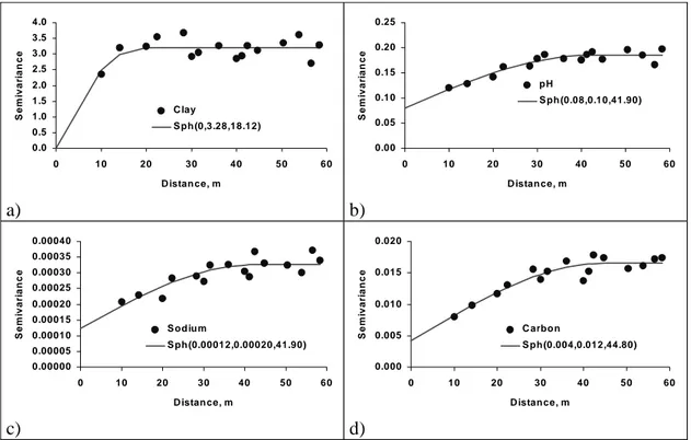
Figure 1 shows the semivariograms for clay, pH, sodium and carbon on the LVa (Ultisol), at 0-10cm depth. The parameters for the models corresponding to the semivariograms shown in figure 1 are in table 1. As it can be seen, the ranges of spatial dependences show a large variation (from 18.12m for clay up to 44.80m for carbon).

The semivariogram for clay content shows a zero nugget effect value a low range of spatial dependence. The zero nugget effect value indicates a very smooth spatial continuity between neighbouring points.

On the other hand, the low range of spatial dependence (18.12m) indicates that this continuity

0.0 0.5 1.0 1.5 2.0 2.5 3.0 3.5 4.0

0 10 20 30 40 50 60

D istan ce, m

Se

mi

v

a

ri

a

nc

e

C lay

S ph (0,3.28,18.12)

a)

0.00 0.05 0.10 0.15 0.20 0.25

0 10 20 30 40 50 60

D istan ce, m

Se

mi

v

a

ri

a

nc

e

pH

S ph (0.08,0.10,41.90)

b)

0.00000 0.00005 0.00010 0.00015 0.00020 0.00025 0.00030 0.00035 0.00040

0 10 20 30 40 50 60

D istan ce, m

S

em

ivar

ian

c

e

S od iu m

S ph (0.00012,0.00020,41.90)

c)

0.000 0.005 0.010 0.015 0.020

0 10 20 30 40 50 60

D istan ce, m

S

em

ivar

ian

c

e

C arbo n

S ph (0.004,0.012,44.80)

d)

disappears very fast. The other three variables (pH, Sodium and Carbon) have larger ranges of spatial dependence (approximately 42m) but have also larger nugget effect values.

The sixth column of table 1 shows the proportion of the nugget effect values to the sill. This is called the correlation ratio, whose closeness to zero indicates the continuity in the spatial dependence.

The knowledge of the spatial variability of organic carbon and pH may be important for understanding the variance structure of crop yield and how they can be related. The LVa soil is of medium texture and has approximately 30% fine sand in the 0-10cm layer.

Figure 1. Semivariogram for some of the chemical properties analyzed, LVa (Ultisol).Numbers in parenthesis are

nugget effect value (Co), C1 and range (a). Sph means spherical model.

Table 1. Parameters for semivariogram spherical models for some of the chemical properties, LVa (Ultisol), shown in figure 1.

Variable C0 C1 a r2 C0/(C0+C1)

Clay 0.00 3.28 18.12 0.9926 0.0000

pH 0.08 0.10 41.90 0.8646 0.4339

Sodium 0.00012 0.00020 41.90 0.7181 0.3773

In this situation, the organic carbon content may be even more important in terms of explaining the variability of crop yield. Spatial variation of clay content, somewhat different from pH and organic carbon, may cause difficulty in the judgment of the yield variability, as the crops somehow integrate these factors over the area. Because of the nature of these attributes with many factors affecting them in different proportions across the landscape, they are so variable from place to place as compared to clay content, as indicated by their correlation ratios.

Remembering that the semivariogram is a result of the mean squared differences between the neighbouring values, the graphs in figure 1 show that values close together are more similar than those farther apart, in the order clay>carbon>sodium>pH. The increase in the semivariance with distance guarantees that statement.

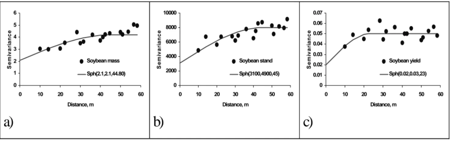
Spatial dependence between neighbouring observations for soybean yield parameters on the LVa (Ultisol) are shown through the semivariograms of to-tal mass, stand and yield in figure 2. One different spherical model was adjusted to each of them. The corresponding parameters for the models fit to the semivariograms are shown in table 2.

The semivariograms for total mass (Figure 2a) and for soybean plant population density(stand) (figure 2b) are somewhat similar in shape, with very similar ran-ges of spatial dependence (44.8m and 45.0m, respectively, table 2).

However, their correlation ratio (sixth column on table 2) is very different (0.5 and 0.38, respectively). Therefore, the plant population may not be the main factor which is affecting the spatial variability of the total soybean mass. Besides, the soybean yield showed an yet much distinct semivariogram, whose range of correlation is about half that of the plant population and total mass.

Naturally, crop yield is a variable that integrates the spatial variability of many other factors such as soil fertility, available water, and including plant population. For this reason, and this small scale (about 1ha) the influence of any factor individually does not show with enough evidence as to reflect in the yield map.

The semivariogram model fit to the experimen-tal values is such that their parameters were chosen in order to minimize the sum of squares of deviation between the model and the actual semivariance values.

0 1 2 3 4 5 6

0 10 20 30 40 50 60 Distance, m

S

em

iva

ri

an

ce

Soybean mass Sph(2.1,2.1,44.80)

a)

0 2000 4000 6000 8000 10000

0 10 20 30 40 50 60 Distance, m

S

em

iva

ri

an

ce

Soybean stand Sph(3100,4900,45)

b)

0 0.01 0.02 0.03 0.04 0.05 0.06 0.07

0 10 20 30 40 50 60 Distance, m

S

em

iva

ri

an

ce

Soybean yield Sph(0.02,0.03,23)

c)

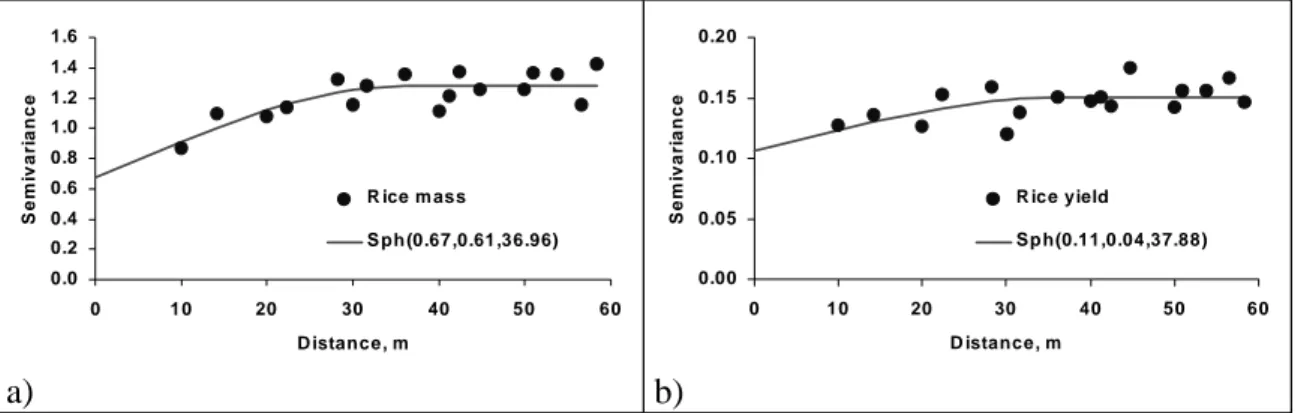
Table 2. Parameters for semivariogram models for soybean and rice yield components, LVa (Ultisol), shown in figures 2 and 3.

Variable C0 C1 a r2 C0/(C0+C1)

Soybean mass 2.10 2.10 44.80 0.6134 0.5000

Soybean stand 3100 4900 45.00 0.5704 0.3875

Soybean yield 0.02 0.03 23.00 0.2163 0.4000

Rice mass 0.67 0.61 36.96 0.6067 0.5229

Rice yield 0.11 0.04 37.88 0.2688 0.7052

Again, the slopes of the fitted models at distances smaller than the correlation range (44.8, 45.0 and 23.0 meters, table 2) guarantee that these attributes have continuity from place to place, and also supports the geostatistical expansion from point observations to a continuous map.

Similarly, the semivariograms for rice yield parameters shown in figure 3, exhibits a structured spatial behaviour. The correlation range for the rice mass is smaller than the corresponding one for soybean, and the range for the semivariogram for rice yield is larger than that of the soybean yield (table 2). On the other hand, rice mass and rice yield seem to have a spatial variability more related to each other, as their semivariograms have more similar parameters when compared to those for the soybean (table 2). That means that the rice yield over the area is closely related to the corresponding total mass. Considering that these two crops were grown on the exact same

field in two consecutive years, the semivariograms for soybean yield (Figure 2c)) and for rice yield (Figure 3b)) express very different variability. The variability for soybean is more continuous at short distances as indicated by the correlation ratio of 0.4 for soybean as compared to 0.7 for rice (table 2). On the other hand, soybean yield loses continuity at shorter distances (23m)

It should also be emphasized that the semivariograms for the yields and components shown in figures 2 and 3, are for the same experimental site as that for pH and organic carbon, shown in figure 1 and that they all have a similar range of correlation somewhere in the neighbourhood of 40 m, except for clay content. This may be an indication that the yield variability may be related to these soil chemical properties, even though the results indicate that the relationship to any factors may change from one crop to the other.

0.0 0.2 0.4 0.6 0.8 1.0 1.2 1.4 1.6

0 10 20 30 40 50 60

D istance, m

S

e

mi

var

ia

nce

R ice m ass

S ph (0.67,0.61,36.96)

a)

0.00 0.05 0.10 0.15 0.20

0 10 20 30 40 50 60

D istance, m

S

e

m

iv

a

ri

ance

R ice yield

Sp h(0.11,0.04,37.88)

b)

Figure 3. Semivariogram for rice yield components, LVa (Ultisol) than rice (37.88m). The reasons for such a change in

variability from one crop to the other can be numerous. First of all, different crops react in distinct ways to the soil conditions, and so, soybean and rice, in addition to that, are leguminous and grass.

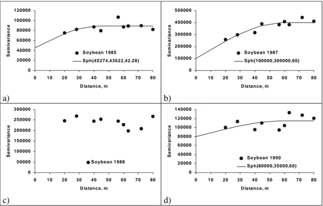
The variability of the soybean and winter crops yield on LRd (Oxisol) is expressed through the semivariograms shown in figure 4 and 5 and the corresponding parameters for the models fit are shown in tables 3 and 4. It can be seen from the difference in the semivariograms that the spatial behaviour of the soybean yield (figure 4) changes from one year to another, probably due to climatic changes favouring crop growth and production in different ways over the field.

For instance, the soybean crop yield in 1988 may be considered to have a pure nugget effect while in 1987 it shows a very well defined spatial structure. The winter crops (Figure 5) have a more simi-lar variability among themselves than the soybean. One of the possible causes for this is that there were less weeds during the winter cropping seasons and

they were less aggressive for the winter cropping seasons.

Figures 6 and 7 show the semivariograms for the leaf chemical analysis and soybean yield together. The corresponding parameters for the models fit to the semivariograms are shown in tables 5 and 6, respectively for figures 6 and 7. The comparison between these semivariograms indicates that the leaf analysis also changes from one year to the other and so does the relationship between the results and crop yield. The semivariograms shown in Figures 6 and 7 are very distinct not only on range of correlation but also in the nugget effect value.

0 20000 40000 60000 80000 100000 120000

0 10 20 30 40 50 60 70 80

D istance, m

S e mi var ia nce

S oybean 1985 S ph(45274,43622,42.28)

a)

0 10 20 30 40 50 60 70 80

D istance, m

S e mi var ia nce

S oybean 1987 S ph(100000,300000,60)

b)

0 10 20 30 40 50 60 70 80

D istance, m

S em iva ri a n ce

S oybean 1988

c)

0 10 20 30 40 50 60 70 80

D istance, m

S em iva ri a n ce

So yb ean 1990 Sp h(80000,35000,60)

d)

Figure 4. Semivariogram for Soybean yield, LRd (Oxisol).

0 1000 2000 3000 4000 5000 6000 7000 8000 9000

0 10 20 30 40 50 60 70 80

D istan ce, m

S em iva ri a n ce

R ye 1986 S ph (2700,4000,65)

a)

0 10 20 30 40 50 60 70 80

D istan ce, m

S em iva ri a n ce

C orn 1986

S p h(450000,1000000,65)

b)

0 10 20 30 40 50 60 70 80

D istan ce, m

S em iva ri a n ce Oats 1987

S ph (10000,30000,50)

c)

0 10 20 30 40 50 60 70 80

D istance, m

S em iva ri a n ce

R ye 1991 S ph (0,87805.9,70)

d)

Table 3. Parameters for semivariogram models for soybean yield at LRd (Oxisol) in four different years, shown in figure 4.

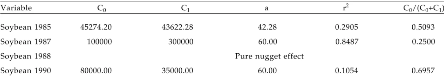
Variable C0 C1 a r2 C0/(C0+C1)

Soybean 1985 45274.20 43622.28 42.28 0.2905 0.5093

Soybean 1987 100000 300000 60.00 0.8487 0.2500

Soybean 1988 Pure nugget effect

Soybean 1990 80000.00 35000.00 60.00 0.1054 0.6957

Table 4. Parameters for semivariogram models for winter crops at the LRd (Oxisol), shown in figure 5.

Variable C0 C1 a r2 C0/(C0+C1)

Rye 1986 2700.0 4000.0 65.00 0.6072 0.4030

Corn 1986 450000 1000000 65.00 0.5021 0.3103

Oats 1987 10000.0 30000.0 50.00 0.5496 0.2500

Rye 1991 0.00 87805.91 70.00 0.7671 0.0000

0.0000 0.0002 0.0004 0.0006 0.0008 0.0010 0.0012 0.0014 0.0016 0.0018

0 10 20 30 40 50 60 70 80 D istance, m

S

em

ivar

ian

ce

P

Sph (0,0.0014,70)

a)

0.0000 0.0002 0.0004 0.0006 0.0008 0.0010 0.0012

0 10 20 30 40 50 60 70 80 D istan ce, m

S

em

ivar

ian

ce

Mg

S ph(0.00025,0.00075,65)

b)

0 200 400 600 800 1000

0 10 20 30 40 50 60 70 80 D istan ce, m

S

e

m

ivar

ia

n

ce

Mn

S ph(50,600,70)

c)

0 20000 40000 60000 80000 100000 120000

0 10 20 30 40 50 60 70 80 D istance, m

S

e

mi

var

ia

n

c

e

So ybean yield 1986 Sp h(50,600,70)

d)

Figure 6. Semivariogram for leaf analysis and Soybean yield, 1985 LRd (Oxisol).

Table 5. Parameters for semivariogram models for some leaf analysis results and soybean yield in 1985 shown in figure 6.

Variable C0 C1 a r2 C0/(C0+C1)

P 0.0 0.0 70.0 0.7115 0.0000

Mg 0.0 0.0 65.0 0.6792 0.2500

Mn 50.0 600.0 70.0 0.5465 0.0769

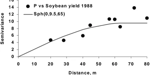
The spatial relationship between P in the leaves and the soybean grain yield in 1988 is shown in the cross semivariogram in figure 8. VIEIRA et al. (1987) found spatial dependence between residual P fertiliser from grapes and the total mass of green manure Crotalaria junceae. The spherical model fitted to the experimental cross semivariances (table 7) with a nugget effect value of 0.0, a sill of 9.5 and a range of 65.0m is shown along with the experimental cross semivariogram values. Thus, it is possible to use this spatial correlation between them and to use cokriging to estimate one of them, for instance, the soybean yield.

VAUCLINet al. (1983) showed that cokriging could be

used for variables that have been sampled in fewer places but the gain in estimation variance with respect to ordinary kriging is small.

The cross semivariogram between Phosphorus in the leaves and yield of soybean for 1986 did not show a clear relationship. This also indicates that the cause of variability may change with time.

The maps obtained through kriging are shown in figures 9 and 10, for rice and soybean yields, respectively. The comparison of these maps may be useful in the interpretation of the results.

Table 6. Parameters for semivariogram models for some leaf analysis results and soybean yield in 1988 shown in figure 7.

Variable C0 C1 a r2 C0/(C0+C1)

P 0.001 0.001 65.0 0.4357 0.5000

Mg 0.0 0.0 65.0 0.5949 0.2143

Soybean yield 1988 130000 260000 60.0 0.5309 0.3333

0.0000 0.0005 0.0010 0.0015 0.0020 0.0025 0.0030

0 10 20 30 40 50 60 70 80

D istan ce, m

S

em

iva

ri

an

c

e

P

S ph(0.001,0.001,65)

a)

0.0000 0.0002 0.0004 0.0006 0.0008 0.0010 0.0012 0.0014 0.0016 0.0018

0 10 20 30 40 50 60 70 80

D istance, m

S

em

iva

ri

an

c

e

Mg

Sp h(0.0003,0.0011,65)

b)

0 100000 200000 300000 400000 500000

0 10 20 30 40 50 60 70 80

D istance, m

S

em

iva

ri

an

c

e

S oyb ean yield 1988

S ph(130000,260000,60)

c)

Figure 7. Semivariogram for leaf analysis and Soybean yield, 1988 LRd (Oxisol).

0 2 4 6 8 1 0 1 2 1 4 1 6

0 1 0 2 0 3 0 4 0 5 0 6 0 7 0 8 0

D is ta n c e , m

S

e

mi

v

a

ri

a

nc

e

P v s S o yb e a n y ie ld 1 9 8 8

S p h (0 ,9 .5,6 5 )

0 20 40 60 80 100 120 140 160 0

20 40 60 80 100 120

300 600 900 1200 1500 1800 2100

a)

0 20 40 60 80 100 120 140 160 0

20 40 60 80 100 120

1800 2200 2600 3000 3400 3800 4200 4600

b)

0 20 40 60 80 100 120 140 160 0

20 40 60 80 100 120

1200 1600 2000 2400 2800 3200 3600 4000

d)

0 20 40 60 80 100 120 140 160 0

20 40 60 80 100 120

400 800 1200 1600 2000 2400 2800

d)

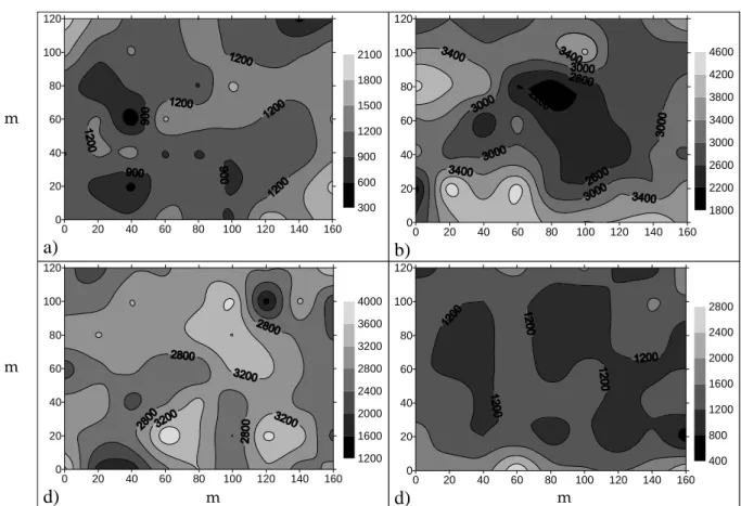
Figure 9. Yield (Mg.ha-1) maps for soybean at LRd, Campinas, SP, Brazil, in 1985 (a), 1987 (b), 1988 (c), and 1990 (d). Table 7. Parameters for cross semivariogram model for leaf analysis P vs Soybean yield in 1988, LRd (Oxisol) shown in figure 8.

Variable C0 C1 a r2 C0/(C0+C1)

P vs Soybean yield 1988 0.0 9.5 65.0 0.2245 0.0000

0 10 20 30 40 50 60 70 80 90 100 0

10 20 30 40 50 60 70 80 90

1.0 1.5 2.0 2.5 3.0

a)

0 10 20 30 40 50 60 70 80 90 100 0

10 20 30 40 50 60 70 80 90

0.8 1.0 1.2 1.4 1.6 1.8

b)

Figure 10. Yield (Mg.ha-1_{) map for rice (a) and for soybean (b) at the LVa, Votuporanga, SP, Brazil.}

m m

m m

m

For instance, there is an area of low yield on the left part of figure 9, which is probably due to compaction where the tractors and machinery make turns. On the other hand, the yield map for soybean (Figure 10), indicates high values for many the regions in which the rice yield map (Figure 9) showed low values. It is possible that the factors affecting rice yield are different from those affecting the soybean.

4. CONCLUSIONS

The existence of spatial dependence allowed the construction of yield maps with known precision using kriging interpolation. This way, visual comparison of yield map for different crops and evaluation of the spatial variability of the yield components and related soil properties was possible. The spatial distribution of rice yield is different from soybean yield. It is possible that the factors affecting the variability of rice yield are not the same than for soybean. The change with time in the cross semivariogram between phosphorus in the leaves and soybean yield indicates that the causes of variability may change with time.

REFERENCES

CAMARGO, O.A.; MONIZ, A.C; JORGE, J.A.; VALADARES, J.M.A.S. Métodos de análise química, mineralógica e física de solos do Instituto Agronômico de Campinas. Campinas: Instituto

Agronô-mico, 1986. 94 p. (Boletim técnico, 106)

HARRIS, J.A. Practical universality of field heterogeneity as a factor influencing plot yields. Journal of Agricultural Research, Washington, v. XIX, n.7, p. 279-314, 1920.

LAL, R. Soil erosion by wind and water problems and prospects. In: LAL, R. (ed.). Soil erosion research methods. Ankeny: Soil Conservation Society of America, 1988. p. 153-185.

MATHERON, G. The theory of regionalized variables and its

application. Fontainebleau: Les Cahiers du Centre de

Morphologie Mathematique, 1971. 56 p. (Fascicule 5)

McBRATNEY, A.B.; WEBSTER, R. Detection of ridge and furrow pattern by spectral analysis of crop yield. International Statistical Review, Voorburb, v. 49, p.49-52, 1981.

McBRATNEY, A.B.; WEBSTER, R.; McLAREN, R.G.; SPIERS, R.B. Regional variation of extractable copper and cobalt in the topsoil of southwest Scotland. Agronomie, Paris, v.2, n.10,

p.969-982, 1982.

MILLER, M.P.; SINGER, M.J.; NIELSEN, D.R. Spatial variability of wheat yield and soil properties on complex hills. Soil Science Society of America Journal, Madison, v.52, p.1133-1141, 1988.

MONTGOMERY, E.G. Experiments in wheat breeding:

experi-mental error in the nursery and variation in nitrogen and yield. Washington: United States Department of Agriculture/Bureau of Plant Industry, 1913. p. 5-61. (USDA Bulletin, 269)

MULLA, D.J. Mapping and managing spatial patterns in soil fertility and crop yield. In: Soil specific crop management. Madison:

Soil Science Society of America, 1993. p. 15-26.

PREVEDELLO, B.M.S. Variabilidade espacial de parâmetros de solo e planta. 1987. 166 p. Tese (Doutorado) - Escola Superior de

Agricultura Luiz de Queiroz, Universidade de São Paulo, Piracicaba.

RAIJ, B. van; QUAGGIO, J.A. Métodos de análise de solo para fins de fertilidade. Campinas, Instituto Agronômico, 31p. 1983. (Boletim técnico, 81).

SALVIANO, A.A.C. Variabilidade de atributos de solo e crotalária júncea em solo degradado do município de Piracicaba – SP. 1966. 91p. Tese (Doutorado) - Escola Superior de Agricultura Luiz de Queiroz, Universidade de São Paulo, Piracicaba.

SARRUGE, J.R.; HAAG, H.P. Análises químicas em plantas.

Piracicaba: Escola Superior de Agricultura Luiz de Queiroz/ Universidade de São Paulo, 1974. 56p.

SNEDECOR, G.W.; COCHRAN, W.G. Statistical methods. 6th

Edition. Ames: Iowa State University Press, 1967. 593 p.

SOUZA, L.S. Variabilidade espacial do solo em sistemas de manejo.

1992. 162p. Tese (Doutorado) - Faculdade de Agronomia/Uni-versidade Federal do Rio Grande do Sul, Porto Alegre.

VAUCLIN, M.; VIEIRA, S.R.; BERNARD, R.; HATFIELD, J.L. Spatial variability of two transects of a bare soil. Water Resources Research, Washington, v.18, n.6, p.1677-1686, 1982.

VAUCLIN, M.; VIEIRA, S.R.; VACHAUD, G.; NIELSEN, D.R. The use of cokriging with limited field soil observations. Soil Science Society of America Journal, Madison, v.47, p.175-184, 1983. VIEIRA, S.R. Uso de geoestatística em estudos de variabilidade espacial de propriedades do solo. In: NOVAIS, R.F. (Ed.). Tópi-cos em Ciência do Solo. Viçosa: Sociedade Brasileira de Ciência do

Solo, 2000. p.1-54.

VIEIRA, S.R. Variabilidade espacial de argila, silte e atributos químicos em uma parcela experimental em um Latossolo Roxo de Campinas (SP). Bragantia,Campinas, v. 57, n. 1, p.181-190, 1997. VIEIRA, S.R.; DE MARIA, I.C. Delineamento experimental e análise estatística na pesquisa em conservação do solo. In: PUIGNAU, J.P.; DENARDIN, J.E.; KOCHHAN, R.A.; MOTTER, D.R.; WALL, P.C. (Eds.). Metodologías parainvestigación en mane-jo de suelos. Montevideo: IICA, 1994, p.3-11 (Diálogos, 39).

VIEIRA, S.R.; DE MARIA, I.C.; CASTRO, O.M.; DECHEN, S.C.F.; LOMBARDI NETO, F. Utilização da análise de Fourier no estudo do efeito residual da adubação em uva na crotalária.

VIEIRA, S.R.; LOMBARDI NETO, F. Variabilidade espacial de potencial de erosão das chuvas do Estado de São Paulo.

Bragantia, Campinas, v. 54, n.2, p. 405-412, 1995.

VIEIRA, S.R.; LOMBARDI NETO, F.; BURROWS, I.T. Mapeamento das precipitações máximas prováveis para o Es-tado de São Paulo. Revista Brasileira de Ciência do Solo,

Campi-nas, v.15, p.93-98, 1991.

VIEIRA, S.R.; NIELSEN, D.R.; BIGGAR, J.W. Spatial variability of field-measured infiltration rate. Soil Science Society of America Journal, Madison, v.45, p.1040-1048, 1981.

VIEIRA, S.R.; NIELSEN, D.R.; BIGGAR, J.W.; TILLOTSON, P.M. The scaling of semivariograms and the kriging estimation.

Revista Brasileira de Ciência do Solo, Viçosa, v. 21, p.525-533, 1997.

VIEIRA, S.R.; REYNOLDS, W.D.; TOPP, G.C. Spatial variability of hydraulic properties in a highly structured clay soil. In: WIERENGA, P.J.; BACHELET, D. (Eds.). VALIDATION OF FLOW AND TRANSPORT MODELS FOR THE UNSATURATED ZONE, 1988, Las Cruces. Proceedings… Las Cruces: Department of Agronomy and Horticulture, New Mexico State University, 1988, p. 471-483. (Research Report 88—SS-04)

WAYNICK, D.D. Variability in soils and its significance to past and future soil investigations. I. Statistical study of nitrification in soils. Agricultural Sciences, Davis, v.3, n.9,