MHD Solar Fluctuations and Solar Neutrinos
N. Reggiani
1, M.M. Guzzo
2, and P.C. de Holanda
31
Faculdade de Matem´atica, Centro de Ciˆencias Exatas Ambientais e de Tecnologias
Pontif´ıcia Universidade Cat´olica de Campinas, 13086-900 Campinas-SP, Brazil 2
Instituto de F´ısica ‘Gleb Wataghin’, Universidade Estadual de Campinas, UNICAMP, 13083-970 Campinas, SP, Brazil 3
The Abdus Salam International Centre for Theoretical Physics, I-34100 Trieste, Italy
Received on 16 June, 2002. Revised version received on 2 July, 2002.
We analyze how solar neutrino experiments could detect time fluctuations of the solar neutrino flux due to magnetohydrodynamic (MHD) perturbations of the solar plasma. We state that if such time fluctuations are detected, this would provide a unique signature of the Resonant Spin-Flavor Precession (RSFP) mechanism as a solution to the Solar Neutrino Problem.
I
Introduction
Assuming a non-vanishing magnetic moment of neu-trinos, active electron neutrinos that are created in the Sun can interact with the solar magnetic field and be spin-flavor converted into sterile nonelectron neu-trinos or into active nonelectron antineuneu-trinos. This phenomenon is called Resonant Spin-Flavor Precession (RSFP). Particles resulting from RSFP interact with solar neutrino detectors significantly less than the orig-inal active electron neutrinos in such a way that this phenomenon can induce a depletion in the detectable solar neutrino flux [1].
If this interaction of the neutrinos with the solar magnetic field is the mechanism that explains the neu-trino deficit on Earth [2]-[6], or, in other words, if the RSFP is the mechanism that solve the solar neutrino problem, solar magnetohydrodynamics (MHD) pertur-bations can lead to time fluctuations of the solar neu-trino flux detected on Earth. This can be easily un-derstood. The solar active electron neutrino survival probability based on the RSFP mechanism crucially depends on the values of four independent quantities. Two of then are related to the neutrino properties: its magnetic moment µν and the squared mass difference of the physical eigenstates involved in the conversion mechanism divided by their energy ∆/4E. The other two quantities are related to the physical environment in which neutrinos are inserted: the magnetic field pro-file B(r) and the electron (and neutron, for Majorana neutrinos) number density distributionN(r) along the neutrino trajectory. MHD affects both the magnetic field profile as well as the matter density and there-fore its effects will strongly influence the RSFP neu-trino survival probability. Indeed we believe that such consequences can be thought as a test to this solution to the solar neutrino problem based on the RSFP mech-anism [7-10].
II
MHD perturbations
The MHD perturbations were calculated deriving the MHD equations near the solar equator, the region rele-vant for solar neutrinos. Using cylindrical coordinates, considering also the effects of gravity, we obtained the Hain-L¨ust equation with gravity [11, 12, 7]:
∂ ∂r
f(r) ∂ ∂r(rξr)
+h(r)ξr = 0 (1) where
f(r) =γp+B 2 o r
(w2
−w2
A)(w2−w2S) (w2−w2
1)(w2−w22)
, (2)
h(r) = ρ0w2−k2B20+g ∂ρ0
∂r
−1
Dgρ 2 0(w
2ρ
0−k2B20)
gH+w 2 r −∂ ∂r 1 Dw 2ρ2
0g(w 2ρ
0−k2B02)
(3)
and
wA2 = k2B2
0 ρ0
, w2S = γp γp+B2
0 k2B2
0 ρ0
, (4)
w2 1,2=
H(γp+B2 0) 2ρ0
1±
1−4 γpk 2B2
0 (γp+B2
0)2H
1/2
,
(5) D=ρ2
0w 4
−H[ρ0w2(γp+B20)−γpk 2B2
0], (6) H =m
2
r2 +k
2 (7)
the pressure, γ = Cp/Cv is the ratio of the specific heats, ρ0 is the equilibrium matter density profile and B0 is the magnetic equilibrium profile in the Sun. In this derivation we considered the equilibrium magnetic profileB0 in the azimuthal direction.
The Hain-L¨ust equation shows singularities when f(r) given in equation (2) is equal to zero, that is, when w2 =w2
A or w2 =w2S, which regions in the w2 space are called Alfv´en and slow continua, respectively. In the interval 0 ≤r ≤ 1 the functionsw2
A and w 2 S take continuous values that define the ranges of the values of w2 that correspond to improper eigenvalues, asso-ciated with localized modes. Eigenvalues of the Hain-L¨ust equation must be searched, therefore, outside the regions where w2 =w2
A or w2 =w2S, and they define the global modes which are associated with magnetic and density waves along the whole radius of the Sun.
For the equations above we considered for the so-lar matter density distribution, ρ0, the standard solar model prediction, that is, approximately monotonically decreasing exponential functions in the radial direction from the center to the surface of the Sun [13]. The density profile was used to calculate the acceleration of gravity. The pressurepis related with the density by the adiabatic equation of state p∼5×10¹⁴ργ, which is obtained from the values of density and temperature of the solar standard model.
The global modes were obtained solving numerically the Hain-L¨ust equation with gravity, imposing appro-priate boundary conditions tob1and ρ1, the magnetic and density perturbations respectively, given by [12]
b1=∇ × (ξ×B0) (8) and
ρ1=∇ · (ρξ). (9) The matter density fluctuations were very con-strained by helioseismology observations. The largest
density fluctuations ρ1 inside the Sun are induced by temperature fluctuationsδT due to convection of mat-ter between layers with different local temperatures. According to an estimate of such an effect [7], we as-sume density fluctuationsρ1/ρ0smaller than 10%. The size of the amplitude b1 is not very constrained by the solar hydrostatic equilibrium, since the magnetic pres-sure B2
0/8π is negligibly small when compared with the dominant gas pressure for the equilibrium profiles considered. Despite this fact, it cannot be arbitrar-ily large when we are solving the Hain-L¨ust equation. This equation is obtained after linearization of the mag-netohydrodynamics equations, which requires that the solution ξ must be very small, |ξ| << 1, so that the non-linear terms can be neglected. Moreover, we must have a clear distinction between the maximum and min-imum magnetic field. In order to satisfy these criteria and have a significant effect, we choose the maximum value of the perturbation such that|b1|/|B0| ∼0.5.
The localized modes are obtained solving the Hain-L¨ust equation in the singularities of the functionf(r). Methods to analytically overcome this singularity sug-gest the inclusion of an arbitrary imaginary constant ia to contour the singularity in such a way thatw2→ w2+ia. Therefore, the magnitude of a, which is di-rectly related with the width of the localized magnetic fluctuation, is an arbitrary value which cannot be elimi-nated from any exact solution of the Hain-L¨ust equation involving the continuum spectrum. Consequently, we adopted the following phenomenological assumption in our calculations: continuum modes introduce Gaussian-shaped magnetic fluctuations centered inrs, with width δr, and amplitude given by a fraction of the equilibrium magnetic field in the position of the singularity, in such a way that the magnitude of the transverse component of the magnetic field, which is the relevant magnetic component for neutrino RSFP, will fluctuate in the fol-lowing way:
⌋
|B⊥(r)|=|B0(r)|+b0|B0(rs)|exp
−
r
−rs δr
2
sin [w(rs)t]. (10)
⌈
where b0 is the amplitude factor, a positive numerical value smaller than 1. We impose that w(rs) = wA or w(rs) =wS and, consequently, generate accordingly a time modulation of the detectable number of neutri-nos coming from the Sun. Note that the shape of the perturbations being exactly Gaussian is not crucial for neutrino RSFP, once solar neutrinos are sensitive to the averaged magnetic field aroundrs.
III
Solar neutrino evolution
If we consider a non-vanishing neutrino magnetic mo-ment, the interaction of such neutrinos with this mag-netic field will generate neutrino spin-flavor conversion which is given by the evolution equations [1]
⌋
id dr
νL νR
=
√
2
2 GFNef f(r)− ∆
4E µν|B⊥(r)|
µν|B⊥(r)| + √
2
2 GFNef f(r) + ∆ 4E
νL νR
where νL (νR) is the left- (right-) handed component of the neutrino field, ∆ is the squared mass difference of the corresponding physical fields, E is the neutrino energy, GF is the Fermi constant, µν is the neutrino magnetic moment and|B⊥(r)|is the transverse
compo-nent of the perturbed magnetic field. Finally, we have Nef f =Ne(r)−Nn(r) for Majorana neutrinos, where Ne(r) (Nn(r)) is the electron (neutron) number density distribution, in which case the final right-handed states νR are active non-electron antineutrinos. For Dirac neutrinos, Nef f =Ne(r)−1/2Nn(r); in this case the right-handed final states are sterile non-electron nos [5]. In this paper we will assume Majorana neutri-nos. Note, however, that sinceNn∼(1/6)Neinside the Sun, the difference of taking Dirac or Majorana neutri-nos is a multiplicative factor of ∼10/11, and does not lead to sensible alterations in our conclusions, which are, in this way, valid for Majorana or Dirac neutrinos. We are considering the standard solar electron number distribution which implies that 10−16 eV
≤
(√2/2)GFNe(r) ≤ 10−12 eV. In order to find appre-ciable spin-flavor neutrino conversion governed by the equations of motion (11), we have to allow the other two relevant quantities in these equations, namely ∆/4E and µν|B⊥(r)|, to be approximately of the same order
of (√2/2)GFNe(r). Assuming the magnetic fields given by equations (12), (13), if we take µν ≈10−11µB (µB
is the Bohr magneton), the quantity µν|B⊥(r)| varies
from approximately 10−14 eV in the central parts of the Sun, to 10−15 eV in the beginning of the convec-tive zone and smaller values than 10−16eV in the solar surface, giving the order of magnitude needed for ap-preciable conversion. For the magnetic field given by (13) and (14) we usedµν = 2×10⁻¹²µB, which gives µν|B⊥(r)| to be of the same order of (
√
2/2)GFNe(r) in the convective zone.
MHD magnetic and density fluctuations,b1 andρ1, induced by global or localized modes, can alter the neu-trino evolution since they can induce time variation of the transverse component of the magnetic field|B⊥(r)|
as well as the matter density Ne(r) appearing in the evolution equation above. Therefore, the MHD fluc-tuations can induce a time variation on the survival probability of the neutrinos, that can be detected in the experiments on Earth.
IV
Localized modes
The effect of the localized modes [7, 8] were estimated calculating the survival probability of an active solar neutrino to reach the solar surface after having inter-acted with the solar magnetic field perturbed by a local-ized MHD wave. In this estimation, we considered for the equilibrium magnetic fields the following profiles:
⌋
B0(r) =
1×10⁶ 0.2 r+0.2
2
G for 0< r≤rconvec BC(r) for r > rconvec ,
(12)
where BC is the magnetic field in the convective zone given by the following profiles:
BIC(r) = 4.88×10 4
1−
r
−0.7 0.3
n
G for r > rconvec (13)
or
BCI(r) = 4.88×10⁴
1 +exp
r
−0.95 0.01
−1
G for r > rconvec (14)
⌈
withn= 2,6 and 8 andrconvec= 0.7. This profile was used by Akhmedov, Lanza and Petcov [14] to show the consistency of the solar neutrino data with the RSFP phenomenon.
Note thatB2
0 < γp, which is related to the fact that the magnetic pressure is negligibly small when com-pared to the gas pressure. Therefore, from Eqs. 4, w2
A ∼ w2S and for the equilibrium profiles considered above, the period of the fluctuation centered at the point of singularity varies from 1 to 10 days.
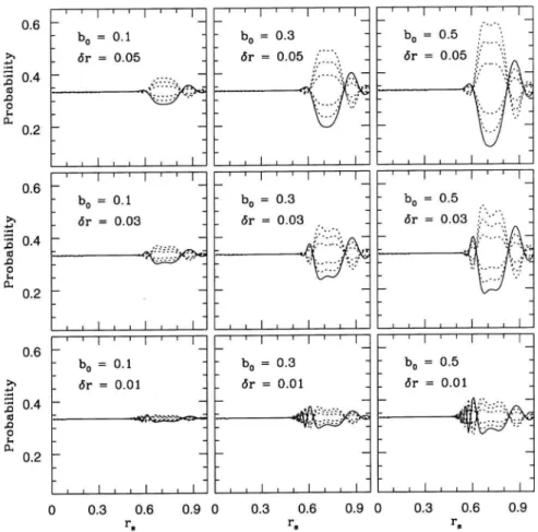
In order to appreciate the relevance of the position of the magnetic fluctuation inside the Sun, its width and amplitude on the solar neutrino survival
Figure 1. The survival probabilityP(νL→νL) of active neutrinos after havinginteracted with the perturbed magnetic field
as a function of the positionrs(normalized by the solar radius) of the Hain-L¨ust equation singularity for the shown values
of the widthδrand the amplitude factorb0. In this figure we assume ∆/4E= 5×10− 16
eV andn= 2 in Eq. (13).
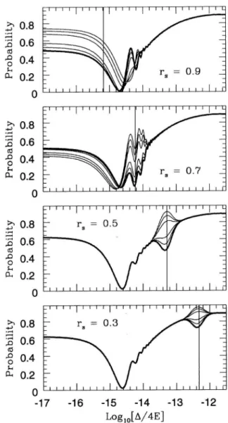
In Fig. 2 it is shown the survival probability as a function of ∆/4E for the indicated values of rs. The magnetic profile used in this figure is given by Eq. (13), withn= 6, and we assumeb0= 0.5 andδr= 0.05. Here the thick continuous line indicates the instant when the magnetic fluctuation is maximal and other lines are suc-cessive time deformations of this fluctuation, with the same assumptions for w(rs)t used in Fig. 1. In these figures, vertical lines indicate the value of ∆/4E cor-responding to a resonance coinciding with the position of the indicated singularityrs. We note that the pres-ence of localized magnetic fluctuations will modify the solar neutrino survival spectrum. In general, low en-ergy neutrinos are less affected by spin-flavor precession than high energy ones. Furthermore, fluctuations of the survival probability are maximal whenrs is close to a resonance region and are well localized in ∆/4E-space
for rs ≤ 0.7. For rs = 0.9 the position of the prob-ability fluctuations in ∆/4E-space is less determined. Nevertheless localized magnetic waves near the solar surface lead to a picture for the survival probability P(νL →νL) which can be easily distinguishable from those ones generated by inner localized waves.
V
Global modes
The global modes [9,10] obtained with the magnetic fields given by equations (12), (13) and (14), used in the analysis of the effect of localized modes, are very similar to each other. So, we present the effect of these modes on the neutrino RSFP phenomenon for just one of these magnetic fields, that we consider a good repre-sentative of the others:
⌋
B0=B0(r) =
1×10⁶ 0.2 r+0.2
2
G for 0< r≤rconvec BC(r) for r > rconvec ,
(15)
whereBC is the magnetic field in the convective zone given by the following profiles: BI
C(r) = 4.88×10⁴
1−
r
−0.7 0.3
n
withn= 6 andrconvec = 0.7.
In order to illustrate the effect of the parametric resonance, we used other magnetic fields that have been used by different authors to solve the solar neutrino problem through the RSFP mechanism [15]:
BCII(r) =
Binitial+ [Brmaxmax−−rBconvecinitial](r−rconvec) for rconvec< r < rmax
Bmax+ [Bmaxrmax−−B1.0f inal](r−rmax) for r > rmax
(17)
⌈
where Binitial = 2.75×10⁵ G, Bmax = 1.18×10⁶ G, Bf inal = 100G, rconvec = 0.65 and rmax = 0.8. Al-though the magnetic field in this configuration seems to be too strong to be present in the convective layer of the Sun, we extend our analysis for this configura-tion because it is very useful to illustrate the parametric resonance effect for different values of the perturbation oscillation length. It is also important to notice that the important quantity for the neutrino evolution is not the magnetic field itself, but the productµν|B⊥(r)|, which
we impose to be of the same magnitude in the Sun con-vective layer for all magnetic field configuration chose here.
We considered also a third field, constant all overr, given by [16]:
B0= 253 kG for 0< r <1.0 (18) For the solar matter density distribution,ρ0, and for the pressurep, we considered the standard solar model prediction, i.e., approximately monotonically decreas-ing exponential functions in the radial direction from the center to the surface of the Sun [13]. The density profile was used to calculate the gravity acceleration.
As the density profile found in [13] is given just until r= 0.95 we have performed our calculations just until this value ofr. The conditions that we imposed onξis over all the calculated values ofr: 0< r <0.95.
In this work we were interested in calculating the eigenfunctions of the Hain-L¨ust equation out of the continua determined by the functions w2 = w2
A and w2 = w2
S. As wA and wS depend linearly on B, the magnetic profiles used were such that there is no value ofrfor whichB is zero, because, ifwA= 0 orwS = 0, this means that the continua extend until w = 0 and in this way all the oscillatory modes below the con-tinua would be killed. Otherwise, it is very reasonable that the magnetic field is non-zero inside the Sun if we choose magnetic profiles which value in the convective zone is ∼105G.
For the magnetic profiles given by (15) and (16) we have possible solutions for w >4.40×10⁻⁵s−1 or w < 5.98×10⁻⁶s−1, which gives a period ofτ <1.65 days or τ > 12.14 days, respectively. For the magnetic profile given by (15) and (17) we havew >4.95×10⁻⁴s−1 or w <5.32×10⁻⁶s−1, which gives a period ofτ <0.15 days or τ > 13.7 days, respectively. For the magnetic profile given by (18) we have w > 6.28×10⁻⁴s−1 or w < 2.56×10⁻⁶s−1, which gives a period τ < 0.11
days orτ >28.5 days, respectively.
Figure 2. The survival probabilityP(νL→νL) as a
func-tion of log10(∆/4E) (∆/4E in units of eV) for the shown
positionrsof the magnetic wave. Vertical lines indicate the
value of ∆/4Ecorrespondingto a resonance coincidingwith the indicated position of the singularityrs. We considered
for the equilibrium magnetic profilen= 6 in Eq. (13).
Figure 3. Profile of a)ξr, after normalization, and b)ρ1/ρ0 and c) b1/B0 that are caused by the magnetohydrodynamic
effect, for the magnetic profiles given by equations [15] and [16] (B0 with n=6), equation [18] (B0 constant) and equations
[15] and [17] (B0 triangular).
assumed. It is important to notice that clearly differ-entξrwavelengths appear for each one of the magnetic fields employed. This will be reflected also in the MHD fluctuations of the matter densityρ1/ρ0 and the mag-netic fieldb1/B0, which are directly calculated fromξr and are shown in the second and third rows of Fig. 3, respectively.
The Hain-L¨ust solutions shown in Fig. 3 are found in the region of the MHD spectrum in which frequen-cies are smaller than the continuum frequenfrequen-cies: w2 < w2
A≈w2S. The period of the solutions found above the continua are smaller thanO(1 sec), very tiny, therefore, to be detected by present experiments.
In Fig. 4 we present the effects on the solar neutrino survival probability when the perturbationsρ1 and b1 are included in the evolution equations (11). In this figure we plot the difference of the survival probability calculated in two different situations: when the effect of the MHD perturbations maximally increases the sur-vival probability and the opposite case when the per-turbations destructively contribute to this probability, decreasing it.
We see that the range of the values of ∆/4E for which this difference is significant varies for each of the magnetic field profile considered. This is a direct conse-quence of the appearance of a parametric resonance [17] in the evolution of the neutrino due to the MHD per-turbations along its trajectory. To understand this ef-fect we have to consider the neutrino oscillation length. When we have a neutrino oscillation length similar to the wavelength of the magnetohydrodynamic perturba-tions, a significant enhancement of the neutrino
chiral-ity conversion occurs. This is the parametric resonance which is clearly observed in the neutrino survival prob-ability. In other words, when the neutrino is evolving, an intense chirality conversion from left to right-handed neutrinos occurs when the magnetic field is increased by the perturbation. On the contrary, when the neutrino oscillation would lead to the opposite chirality conver-sion from right to left neutrino, this coincides with a period of lower magnetic field, and this conversion is suppressed. If the perturbation wavelength is very dif-ferent from the neutrino oscillation length than this ef-fect will not be relevant and we can understand the behavior of Fig. 4 far from the peaks.
VI
Observing MHD fluctuations
in solar neutrino detectors
Figure 4. Amplitude ∆P of the survival probability in func-tion of ∆m/4Efor the magnetic profiles given by equations [15] and [16] (B0 with n=6), equation [18] (B0 constant)
and equations [15] and [17] (B0 triangular).
sensitive to such fluctuations. So, it is necessary to con-sider [10] the detectors that operate in a real time basis and that have a low threshold in the neutrino energy, like Borexino [19], Hellaz [20] and Heron [21].
The Borexino experiment[19]: this experiment will be able to measure the Berilium line neutrinos, in a real time basis. Since the Berilium neutrinos have a fixed energy (E = 0.863 MeV), it is quite easy to predict the time dependence of the neutrino signal in Borexino for a given ∆. Fixing the neutrino energy and taking the magnetic field normalization fB0 = 5, within 99% C.L. no reasonable time fluctuation will be felt by this experiment.
This behavior happens for the three magnetic fields given by (15), (16), (17) and (18), and this can be un-derstood analysing the properties of theses solutions to the solar neutrino problem. In this scenario, we need a strong suppression of the7Beneutrinos (similar to the small mixing angle solution in MSW scenario) in or-der to accommodate both results from Homestake and Gallium experiments (Sage, Gallex, GNO). So, for the 7Beneutrino line we must have a completely adiabatic transition, which makes this line very stable in front of perturbations on the magnetic field profile.
But although we can not use MHD perturbations to test the RSFP solution in Borexino, it has been re-cently discussed [22] how the low value of the expected rate of the Berilium line neutrinos on this experiment would be a clear indication of the RSFP mechanism.
The experiments Hellaz [20] and Heron [21]: these experiments will utilize the elastic reaction, νe,µ,τ + e− →ν
e,µ,τ +e−, for real-time detection in the energy
region dominated by thepp and7Be neutrinos. They will both measure the energy of the recoil electron and the overall rate. These low energy neutrinos are the most abundant solar neutrinos, and the prediction of their flux is the one which carries less uncertainty, be-cause of the correlation of these neutrinos with the solar luminosity. Since the MHD fluctuations we found in [9] appear to be affecting neutrinos with an energy range of the order of the pp-neutrinos energy, maybe Hellaz and/or Heron would be able to feel the time fluctu-ations on the neutrino signal generated by the MHD fluctuations.
Since we expect something around ∼ 7 pp-events/day on experiments like Hellaz or Heron we can see that, for one year (365 days, or∼2500 events) of data taking, in principle it is possible to distinguish such fluctuations in Hellaz experimental results.
Acknowledgments
The authors would like to thank Funda¸c˜ao de Am-paro `a Pesquisa do Estado de S˜ao Paulo (FAPESP) and Conselho Nacional de Desenvolvimento Cient´ıfico e Tecnol´ogico (CNPq) for financial support.
References
[1] A. Cisneros, Astro. & Space Sci.10, 87 (1971); M.B.
Voloshin, M.I. Vysotskii, and L.B. Okun, Yad. Fiz.44,
677 (1986) [Sov. J. Nucl. Phys.44, 440 (1986)]; C.S.
Lim and W.J. Marciano, Phys. Rev. D37, 1368 (1988);
E.Kh. Akhmedov, Phys. Lett. B213, 64 (1988); A.B.
Balantekin, P.J. Hatchell, and F. Loreti, Phys. Rev. D 41, 3583 (1990); J. Pulido, Phys. Rep. 211, 167
(1992); E.Kh. Akhmedov, A. Lanza, and S.T. Petcov, Phys. Lett. B303, 85 (1993); P.I. Krastev, Phys. Lett.
B303, 75 (1993).
[2] K. Lande et al., (Homestake Collaboration), Astro-phys. J.496, 505 (1998).
[3] M. Altmannet al. (GNO Collaboration), Phys. Lett. B490, 16 (2000); C. Cattadori on behalf of GNO
Col-laboration, talk presented at TAUP2001, 8-12 Septem-ber 2001, Laboratori Nazionali del Gran Sasso, Assergi, Italy.
[4] D. N. Abdurashitov et al., (SAGE Collaboration), Nucl. Phys. (Proc. Suppl.) 91, 36 (2001); Latest
re-sults from SAGE homepage:
http://EWIServer.npl.washington.edu/SAGE/.
[5] S. Fukuda et al. (SuperKamiokande Collaboration), Phys. Rev. Lett.86, 5651 (2001); ibid, Phys. Rev. Lett. 865656 (2001).
[6] Q. R. Ahmadet al. (SNO Collaboration), Phys. Rev. Lett.87, 071301 (2001).
[7] M.M. Guzzo, N. Reggiani, and J.H. Colonia, Phys. Rev. D56, 588 (1997).
[9] N. Reggiani, M. M. Guzzo J. H. Colonia-Bartra, and P. C. de Holanda, Eur. Phys. J. C12269 (2000).
[10] M.M. Guzzo, P.C. de Holanda, and N. Reggiani, “MHD fluctuations and Low Energy Solar Neutrinos”, to ap-pear in Eur. Phys. J. C (2002).
[11] E.R. Priest, Solar Magnetohydrodynamics, (D.Reidel PublishingCompany, 1987).
[12] J.P. Goedbloed, Physica 53, 412 (1971); J.P.
Goed-bloed and P. H. Sakanaka, Phys. Fluids17, 908 (1974).
[13] J. N. Bahcall and R. K. Ulrich, Rev. Mod. Phys. 60,
297 (1988); J. N. Bahcall and M. H. Pinsonneault, Rev. Mod. Phys. 64, 885 (1992); J. N. Bahcall, Neutrino
Astrophysics (Cambridge University Press, Cambridge, England, 1989); J. N. Bahcall, S. Basu, and M.H. Pin-sonneault, Astrophys. J.555, 990 (2001).
[14] E.Kh. Akhmedov, A. Lanza, and S.T. Petcov, Phys. Lett. B303, 85 (1993).
[15] M.M. Guzzo and H. Nunokawa, “Current status of the Resonant Spin-flavor Solution to the solar neutrino problem”, HEP-PH/9810408.
[16] H. Minakata and H. Nunokawa, Phys. Rev. Lett. 63,
121 (1989); A. B. Balantekin, P. J. Hatchell, and F. Loreti, Phys. Rev. D 41, 3583 (1990); H. Nunukawa
and H. Minakata, Phys. Lett. B314, 371 (1993).
[17] V.K. Ermilova, V.A. Tsarev, and V.A. Chechin, Kr. Soob, Fiz., Lebedev Inst. 5, 26 (1986); E.
Akhme-dov, Yad. Fiz.47, 475 (1988); P.I. Krastev and A.Yu.
Smirnov, Phys. Lett. B226, 341 (1989).
[18] W. Hampel et al. (GALLEX Collaboration), Phys. Lett. B447, 127 (1999).
[19] S. Malvezzi, Nucl.Phys. B (Proc. Suppl.) 66, 346
(1998).
[20] T. Patzak, Nucl.Phys. B (Proc. Suppl.)66, 350 (1998).
[21] R. E. Lanou, Nucl. Phys. Proc. Suppl. 77 (1999) 55-63; Proceedings of the 8th International Workshop on Neutrino Telescopies (Venice, Italy, 1999), ed. by M. Baldo Ceolin, Vol.I, page 139.
![Figure 3. Profile of a) ξ r , after normalization, and b) ρ 1 /ρ 0 and c) b 1 /B 0 that are caused by the magnetohydrodynamic effect, for the magnetic profiles given by equations [15] and [16] (B 0 with n=6), equation [18] (B 0 constant) and equations [15]](https://thumb-eu.123doks.com/thumbv2/123dok_br/18979910.456657/6.892.233.731.95.468/profile-normalization-magnetohydrodynamic-magnetic-profiles-equations-equation-equations.webp)
![Figure 4. Amplitude ∆P of the survival probability in func- func-tion of ∆m/4E for the magnetic profiles given by equations [15] and [16] (B 0 with n=6), equation [18] (B 0 constant) and equations [15] and [17] (B 0 triangular).](https://thumb-eu.123doks.com/thumbv2/123dok_br/18979910.456657/7.892.84.426.95.466/amplitude-survival-probability-magnetic-profiles-equations-equations-triangular.webp)
