Dark Energy and Some Alternatives: a Brief Overview
J. S. Alcaniz
Departamento de Astronomia, Observat´orio Nacional, 20921-400, Rio de Janeiro – RJ, Brazil
Received on 10 August, 2006
The high-quality cosmological data, which became available in the last decade, have thrusted upon us a rather preposterous composition for the universe which poses one of the greatest challenges theoretical physics has ever faced: the so-called dark energy. By focusing our attention on specific examples of dark energy scenarios, we discuss three different candidates for this dark component, namely, a decaying vacuum energy or time-varying cosmological constant [Λ(t)], a rolling homogeneous quintessence field (Φ), and modifications in gravity due to extra spatial dimensions. As discussed, all these candidates [along with the vacuum energy or cosmological constant (Λ)] seem somewhat to be able to explain the current observational results, which hampers any definitive conclusion on the actual nature of the dark energy.
Keywords: Dark energy; Cosmological constant; Extra dimensions
I. INTRODUCTION
According to Einstein’s general theory of relativity, the dy-namic properties of a given space-time are fully determined by its total energy content. In the cosmological context, for instance, this amounts to saying that in order to understand the space-time structure of the Universe one needs to iden-tify the relevant sources of energy as well as their contribu-tions to the total energy momentum tensorTµν. Matter fields (e.g., baryonic matter and radiation), are obvious sources of energy. Nevertheless, according to current observations, two other components, the so-called dark matter and dark energy (or dark pressure), whose origin and nature are completely unknown thus far, are governing the late time dynamic prop-erties of our Universe. In the standard lore, the later actor plays a special role because it is supposed to be driving the current cosmic acceleration.
Dark energy has been inferred from a number of indepen-dent astronomical observations, which includes distance mea-surements of type Ia supernovae (SNe Ia) [1–3], estimates of the age of the Universe [4], measurements of the Cosmic Mi-crowave Background (CMB) anisotropies [5, 6], and cluster-ing estimates [7]. While the combination of the two latter results suggests the existence of a smooth component of en-ergy that contributes with≃3/4 of the critical density, SNe Ia observations require such a component to have a negative pressure, which generates repulsive gravity and accelerates the cosmic expansion. In addition to these recent observa-tional results, the astonishing success of the inflationary Cold Dark Matter (CDM) paradigm in explaining high precision measurements of CMB anisotropy, galaxy clustering, the Lyα forest, gravitational lensing and other astrophysical phenom-ena can also be thought of as an indirect but important evi-dence for the existence of a dominant repulsive dark energy component
In this short contribution we review some aspects of the so-called dark energy problem. This paper does not aim to be (and is far from being) an exhaustive or complete account of the problem (for that end we refer the reader to Ref. [8]). Here, we focus our attention on three possible mechanisms ca-pable of explaining the current cosmic acceleration, namely, a
decayingΛterm, the potential energy density associated with a dynamical scalar field and modifications in gravity due to extra dimensions effects. As discussed below, all these possi-bilities (together with the standard cosmological constantΛ) seem somewhat to explain the current observational results, which makes the nature of dark energy a completely open question nowadays in Cosmology.
II. COSMOLOGICAL CONSTANT AND DARK ENERGY
There is no doubt that the simplest and most theoretically appealing candidate for dark energy is the cosmological con-stant (Λ), whose presence modifies the Einstein field equa-tions (EFE) to (throughout this paper we work in units where the speed of lightc=1)
Rµν−1
2gµνR=8πGTµν+Λgµν. (1) Physically, Λ acts as an isotropic and homogeneous source with a constant equation of state (EoS)wΛ≡pΛ/ρΛ=−1, whereρΛ≡Λ/8πG1. From a more fundamental viewpoint, a physical basis for the cosmological constant remained un-clear until 1967, when Zel’dovich [9] showed thatΛis related to the zero-point vacuum fluctuations of fields and that those must respect Lorentz invariance so thatTµν=−ρΛgµν. For-mally, the zero-point energy of a quantum field (thought of as a collection of an infinite number of harmonic oscillators in momentum space) must be infinity. If, however, we sum over the zero-point mode energies up to a certain ultraviolet momentum cutoffkc(so that the theory under consideration is
1The simplest way to see how the cosmological term may lead to an
accel-erating expansion in a Friedmann-Robertson-Walker (FRW) universe with pressureless matter componentρmandΛis by means of the Raychaudhury
equation, i.e.,aa¨=−4πG
3 ρm+Λ3 or, equivalently,f=−
GM r2 +
Λ
3r. Clearly,
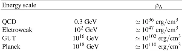
TABLE I: Expected contribution to the vacuum energy.
Energy scale ρΛ
QCD 0.3 GeV ≃1036erg/cm3
Eletroweak 102GeV ≃1047erg/cm3
GUT 1016GeV ≃10102erg/cm3
Planck 1018GeV ≃10110erg/cm3
still valid), we find
ρΛ∼k4c. (2)
By considering the above expression, we show in Table I the expected contribution to the vacuum energy for some funda-mentalenergy scales in nature. The ratio of the values ap-pearing in the third column of Table I to the current obser-vational estimate ofρΛ, i.e.,|ρobsΛ | ∼10−10 erg/cm3, ranges from 46-120 orders of magnitude and is the origin of the fa-mous discrepancy between theoretical and observational es-timates for Λ, the so-called cosmological constant problem (see [10] for a review on this topic). From these arguments one may conclude that although cosmological models with a relicΛterm (ΛCDM) are extremely successful from the ob-servational viewpoint, the fine-tunning problem involving the vacuum energy density andΛseem to hamper any definitive conclusion on the cosmological constant as the actual nature of the mechanism behind cosmic acceleration (see [11] for a broader discussion on this issue).
A. Time-varying Cosmological Constant
A phenomenological attempt at alleviating the above prob-lem is allowing Λto vary2. Cosmological scenarios with a time-varying or a dynamicalΛterm were independently pro-posed almost twenty years ago in Ref. [12] (see also [13–15]). In order to build up aΛ(t)CDM scenario, we first note that according to the Bianchi identities, the Einstein equations (1) implies thatΛis necessarily a constant either ifTµν=0 or if Tµνis separately conserved, i.e.,uµTµν;ν=0. In other words, this amounts to saying that
1. vacuum decay is possible only from a previous exis-tence of some sort of non-vanishing matter and/or radi-ation;
2. the presence of a time-varying cosmological term re-sults in a coupling betweenTµνandΛof the type
uµTµν;ν=−uµ( Λgµν
8πG);ν. (3)
2Strictly speaking, in the context of classical general relativity any
addi-tionalΛ-type term that varies in space or time should be thought of as a newtime-varying fieldand not as a cosmological constant. Here, however, we adopt the usual nomenclature of time-varying or dynamicalΛmodels.
To proceed further, one must now specify the functionΛ(t). However, in the absence of a natural guidance from funda-mental physics on a possible time variation of the cosmolog-ical constant most of the decay laws discussed in the litera-ture are phenomenological (based on dimensional, black hole thermodynamics arguments, among others. See, e.g., [15] and references therein). In this regard, a still phenomenolog-ical but very interesting step toward a more realistic decay law was recently discussed in Ref. [16] (see also [17]), in which the time variation ofΛis deduced from the effect it has on the CDM evolution. The qualitative argument is the fol-lowing: since vacuum is decaying into CDM particles, CDM will dilute more slowly compared to its standard evolution, ρm∝a−3. Thus, if the deviation from the standard evolution is characterized by a constantε, i.e.,
ρm=ρmoa−3+ε, (4) Eq. (3) yields
ρΛ=ρ˜Λo+ ερmo 3−εa
−3+ε, (5)
whereρmois the current CDM energy density,ais the cosmo-logical scale factor, ˜ρΛois an integration constant, and ther-modynamic considerations restrictεto be≥0 [17] (a similar decay law is also obtained from renormalization group run-ningΛarguments [18]). Note that, differently from previous vacuum decay scenarios, in which the universe is either al-ways accelerating or alal-ways decelerating from the onset of matter domination to today, the presence of the residual term ˜
ρΛoin Eq. (5) makes possible a transition from an early de-celerated to a current accelerating phase, as evidenced by SNe Ia observations [19] (see Fig. 1a). Note also that, in the case of vacuum decay into photons3, the primordial nucleosynthe-sis arguments discussed in Refs. [20] (more specifically the bounds from the primordial mass fraction of helium4He and the primordial abundance by number of deuterium D/H) may be no longer valid since even for small values of the parameter εthe residual term ˜ρΛomay account not only for the current cosmic acceleration but also for the recent estimates of the total age of the Universe.
If vacuum is really transferring energy to the CDM com-ponent, the immediate question one may ask is where exactly the vacuum energy is going to or, in other words, where the CDM particles are storing the energy received from the vac-uum decay process. In principle, since the energy density of the CDM component isρ=nm, there are at least two possibil-ities, namely, the current of CDM particles has a source term Nα;α=ψ (while the proper mass of CDM particles remains constant) or the mass of the CDM particles is itself a time-dependent quantitym(t) =moa(t)ε (while the total number of CDM particles, N=na3, remains constant). The former
3If vacuum decays into relativistic particles, all the 3’s in Eqs. (4) and (5)
0 1 2 3 4 -0.4
-0.2 0.0 0.2 0.4
Acceleration Deceleration
ε = 0.05 ε = 0.05 ε = 0.05 ε = 0.05 ε = 0.10 ε = 0.10 ε = 0.10 ε = 0.10 ε = 0.20 ε = 0.20 ε = 0.20 ε = 0.20 Λ Λ Λ ΛCDM
Decel
er
at
ion Par
am
et
er
Redshift
0.0 0.1 0.2 0.3 0.4
0.0 0.1 0.2 0.3 0.4
SNe + Clusters + CMB
Ω Ω Ω Ωm
εεεε
FIG. 1:Left:The deceleration parameter as a function of redshift for some selected values ofε. In all curves a baryonic content corresponding to ≃4.4% of the critical density has been considered. Right: The planeΩm−εfor theΛ(t)CDM scenario. The curves correspond to
confidence regions of 68.3%, 95.4% and 99.7% for a joint analysis involving SNe Ia, Clusters and CMB data. The best-fit parameters for this analysis areΩm=0.27 andε=0.06, with reducedχ2min/ν≃1.14(Figures taken from [17]).
possibility is the traditional approach for the vacuum decay process whereas the latter constitutes a new example of the so-called VAMP4-type scenarios, in which the interaction of CDM particles with the dark energy field imply directly in an increasing of the mass of CDM particles (see, e.g., [21] and references therein for more about VAMP models).
In Fig. 1b we compare the aboveΛ(t)CDM scenario with the standard one (ΛCDM), which is formally recovered for ε=0. We use to this end some of the most recent cosmo-logical observations, i.e., the latest Chandra measurements of the X-ray gas mass fraction in 26 galaxy clusters, as pro-vided by Allen et al. [22] along with the so-calledgoldset of 157 SNe Ia, recently published by Riess et al. [2], and the estimate of the CMB shift parameter [6]. In our analy-sis, we also include the current determinations of the baryon density parameter, as given by the WMAP team [6], i.e., Ωbh2=0.0224±0.0009 and the latest measurements of the Hubble parameter,h=0.72±0.08, as provided by the HST key project [23] (we refer the reader to [24] for more details on this statistical analysis). The contours stand for confidence regions (68.3%, 95.4% and 99.7%) in the planeΩm−ε. Note that, although the limits on the parameterεare very restrictive, the analysis clearly shows that the decaying vacuum scenario discussed above constitutes a small but significant deviation from the standardΛCDM dynamics (as mentioned earlier the standardΛCDM model is very successful from the observa-tional viewpoint so that large deviation from its dynamics are not expected). The best-fit parameters for this analysis are Ωm=0.27 and ε=0.06, with the relativeχ2min/ν≃1.14 (ν is defined as degrees of freedom). Note that this value of
4VAriable Mass Particles
χ2
min/νis similar to the one found for the so-called “concor-dance model” by using SNe Ia data only, i.e.,χ2
min/ν≃1.13 [2]. At 95.4% c.l. we also found Ωm =0.27±0.05 and ε=0.06±0.10. We expect that upcoming observational data along with new theoretical developments will be able to con-firm or notΛ(t)CDM models as realistic dark energy scenar-ios.
III. QUINTESSENCE
If the cosmological term is null or it is not decaying in the course of the expansion, something else must be caus-ing the Universe to speed up. The next simplest approach toward constructing a model for an accelerating universe is to work with the idea that the unknown, unclumped dark en-ergy component is due exclusively to a minimally coupled scalar fieldΦ(quintessence field) which has not yet reached its ground state and whose current dynamics is basically de-termined by its potential energyV(Φ). This idea has received much attention over the past few years and a considerable ef-fort has been made in understanding the role of quintessence fields on the dynamics of the Universe [25]. Examples of quintessence potentials are ordinary exponential functions V(Φ) =V0exp(−λΦ)[26–28], simple power-laws of the type V(Φ) =V0Φ−n[29], combinations of exponential and sine-type functionsV(Φ) =V0exp(−λΦ)[1+Asin(−νΦ)] [30], among others (see, e.g., [8, 25] and references therein).
-0.5 0.0 0.5 1.0 1.5 2.0 -1.0
-0.9 -0.8 -0.7 -0.6 -0.5
α α α
α
= 0.0
α α α
α
= 0.2
α α α
α
= 0.8
α α α
α
= 1.0
α α α
α
= 1.5
w(
z)
Redshift
-0.5 0.0 0.5 1.0 1.5
-1.0 -0.5 0.0 0.5
acceleration deceleration
α
αα
α
= 0.0
α
αα
α
= 0.2
α
αα
α
= 0.8
α
αα
α
= 1.0
Λ
CDM
q(
z)
Redshift
FIG. 2: Left: The planew(z)−z. Note thatw(z)reduces to a constant EoSw≃ −0.96 [λ=O(10−1)] in the limitα→0 while∀α=0
it was−1 in the past and→+1 in the future. Right: The deceleration parameter as a function of the redshift for selected values ofαand Ωm,0=0.27. For values ofα=0 the cosmic acceleration is a transient phenomenon. In particular, forα=1.0 the transition redshifts happen
atza/d≃ ±0.77(Figures taken from [33]).
and the observable structure of the Universe. If, however, it is desirable a more complete connection between the physical mechanism behind dark energy and a fundamental theory of nature, one must bear in mind that an eternally accelerating universe, a rather generic feature of quintessence scenarios, seems not to be in agreement with String/M-theory (possi-ble candidates of a model for quantum gravity) predictions, since it is endowed with a cosmological event horizon which prevents the construction of a conventional S-matrix describ-ing particle interactions [31]. Although the transition from an initially decelerated to a late-time accelerating expansion is becoming observationally established [19], the duration of the accelerating phase, depends crucially on the cosmological scenario and, several models, which includes our current stan-dardΛCDM scenario, imply an eternal acceleration or even an accelerating expansion until the onset of a cosmic singu-larity (e.g., the so-called phantom cosmologies [32]). This dark energy/String theory conflict, therefore, leaves us with the formidable task of either finding alternatives to the con-ventional S-matrix or constructing a quintessence model of the Universe that predicts the possibility of a transient acceler-ation phenomenon. In this regard, an interesting quintessence scenario whose accelerating phase is a transient phenomenon has been proposed in Ref. [33]. In what follows, we highlight some of its features.
Let us first consider a homogeneous, isotropic, spatially flat cosmologies described by the FRW flat line element. The ac-tion for the model is given by
S= m 2 pl 16π
d4x√−g[R−1 2∂
µΦ∂
µΦ−V(Φ) +
L
m], (6) whereR is the Ricci scalar and mpl ≡G−1/2 is the Planck mass. The scalar field is assumed to be homogeneous, suchthatΦ=Φ(t)and the Lagrangian density
L
mincludes all mat-ter and radiation fields.By combining the following ansatz on the scale factor derivative of the energy density
1 ρΦ
∂ρΦ ∂a =−
λ
a1−2α (7)
with the conservation equation for the quintessence compo-nent, i.e., ˙ρΦ+3H(ρΦ+pΦ) =0, the expressions for the scalar field and its potential can be written as
Φ(a)−Φ0= 1 √
σln1−α(a), (8)
and
V(Φ) =f(α;Φ)ρΦ,0exp
−λ√σ
Φ+α √
σ
2 Φ
2
. (9)
In the above expressionsαandλare positive parameters,Φ0 is the current value of the fieldΦ,σ=8π/λm2pl, f(α;Φ) = [1−λ6(1+α
√
σΦ)2], and the generalized function ln 1−ξ, de-fined as ln1−ξ(x)≡(xξ−1)/ξ, reduces to the ordinary loga-rithmic function in the limitξ→0 [34]. The important aspect to be emphasized at this point is that in the limitα→0 Eqs. (8) and (9) fully reproduce the exponential potential studied by Ratra and Peebles in Ref. [26], while∀α=0 the scenario described above represents a generalized model which admits a wider range of solutions.
The EoS for this quintessence component, i.e.,
w(a) =−1+λ 3a
2α,
(10)
λ=0.1. The EoS above (which must lie in the interval−1≤ w(a)≤1) is an increasingly function of time, being ≃ −1 in the past, ≃ −0.96 today, and becoming more positive in the future (0 ata=301/2α and 1/3 ata=401/2α). Such a behavior is typical of the so-calledthawingfields, as discussed in Refs. [35]. For this kind of fields, Ref. [35] also provides the following constraint
1+w<w′<3(1+w), (11) wherew′=dw/dlna. Note that, if it is natural to impose such a constraint at the epoch when dark energy starts becoming important, i.e., atz≃1, then the above interval forw′can be translated into the following bounds on the indexα
1/2<α<3/2. (12)
Clearly, for all the values ofαranging in the above interval, the cosmic acceleration is a transient phenomenon since the quintessence fieldΦwill behave more and more as an attrac-tive matter field. In order to better visualize this transient behavior, we show in Fig. (2b) the deceleration parameter, q=−aa¨/a˙2, as a function of the redshift for some values of the indexαandΩm,0=0.27. As can be seen from this figure, ∀α=0 the Universe was decelerated in the past, began to ac-celerate atza1, is currently accelerated but will eventually decelerate in the future. Note also that, while the accelera-tion redshift za depends very weakly on the value of α, the deceleration redshiftzdis strongly dependent, with the latter transition becoming more and more delayed as α→0. As mentioned earlier, a cosmological behavior like the one de-scribed above seems to be in agreement with the requirements of String/M-theory (as discussed in Refs. [31]), in that the current accelerating phase is a transitory phenomenon5. As one may also check, the cosmological event horizon, i.e., the integral
da/a2H(a)diverges for this transient scalar-field-dominated universe, thereby allowing the construction of a conventional S-matrix describing particle interactions within the String/M-theory frameworks. A typical example of an eternally accelerating universe, i.e., theΛCDM model, is also shown in Fig. (2b) for the sake of comparison.
IV. EXTRA DIMENSIONS
So far we have discussed the phenomenon of cosmic accel-eration as the result of unknown physical processes involving new fields in high energy physics. However, another possi-ble route to deal with this darkpressureproblem could be a modification in gravity instead of any adjustment to the en-ergy content of the Universe. This idea naturally brings to light another important question at the interface of fundamen-tal physics and cosmology: extra dimensions. As is well
5Another interesting example of transient acceleration is provided by the
brane-world scenarios discussed in Ref. [36] and the generalized EoS of Ref. [37]).
known the existence of extra dimensions is required in var-ious theories beyond the standard model of particle physics, especially in theories for unifying gravity and the other fun-damental forces, such as String or M theories6. Extra dimen-sions may also provide a possible explanation for the so-called hierarchy problem, i.e., the huge difference between the elec-troweak and Planck scales [mpl/mEW ∼1016] [39]. In this regard, an interesting scenario was proposed by Randall and Sundrum who showed that, if our 3-dimensional world is em-bedded in a 4-dimensional anti-de-Sitter bulk, gravitational excitations are confined close to our sub-manifold, giving rise to the familiar 1/r2law of gravity [40].
In the cosmological context, the role of extra spatial di-mensions is translated into the so-called brane world (BW) cosmologies [41]. Many attempts to observationally detect or distinguish brane effects from the usual dark energy physics have been recently discussed in the literature. In Ref. [36], for instance, Sahni and Shtanov investigated a class of BW models which admit a wider range of possibilities for the dark pressure than do the usual dark energy scenarios, while Maia et al., in Ref. [42], showed that the dynamics of a dark energy component parametrized by a constant EoS (w) can be fully described by the effect of the extrinsic curvature of a FRW universe embedded into a 5-dimensional, constant curvature de-Sitter bulk.
Another interesting BW scenario is the one proposed by Dvali et al. [43], widely refered to as DGP model (see also [44] for a recent review on the DGP phenomenology). It de-scribes a self-accelerating 5-dimensional BW model with a noncompact, infinite-volume extra dimension whose dynam-ics of gravity is governed by a competition between a 4-dimensional Ricci scalar term, induced on the brane, and an ordinary 5-dimensional Einstein-Hilbert action, i.e.,
S=M 3 (5) 2
d5y
|g(5)|R(5)+m 2 pl 2
d4x|g|R, (13) whereM(5) denotes the 5-dimensional reduced Planck mass. The Friedmann equation which comes from this gravitational action coupled to matter on the brane take the form [45]
ρ 3M2pl+
1 4r2
c + 1
2rc 2
=H2+ k
R(t)2, (14) whereρis the energy density of the cosmic fluid,k=0,±1 is the spatial curvature andrc=M2pl/2M53is the crossover scale defining the gravitational interaction among particles located on the brane. For scales below the crossover radiusrc(where the induced 4-dimensional Ricci scalar dominates), the gravi-tational force experienced by two punctual sources is the usual 4-dimensional 1/r2force, whereas for distance scales larger
6Examples of modified gravity models also include scenarios with higher
FIG. 3:Left:Probability contours at 68.3%, 95.4% and 99.7% confidence levels forΩmversusΩrcin the DGP model from the gold sample of
SN Ia data (solid contours) and in conjunction with the SDSS baryon acoustic oscillations (coloured contours). The upper-left shaded region represents the “no-big-bang” region, the thick solid line represents the flat universe and accelerated models of the universe are above the the dashed line. The best fit happens atΩm=0.272 andΩrc=0.211.Right:The same as in the previous Panel for an analysis involving the first
year SNLS data (solid contours) and in conjunction with the SDSS baryon acoustic oscillations (coloured contours). The best fit happens at Ωm=0.265 andΩrc=0.216(Figures taken from [48]).
thanrcthe gravitational force follows the 5-dimensional 1/r3 behavior7. From the above equation it is also possible to de-fine the density parameter associated with the crossover radius rc, i.e.,
Ωrc=1/4r
2
cHo2. (15) Note that estimates ofΩrcmeans estimates on the length scale
rc. As shown by several authors [46], for values ofrc≃Ho−1, the presence of an infinite-volume extra dimension as de-scribed above leads to a late-time acceleration of the Universe, in agreement with most of the current distance-based cosmo-logical observations8.
In Fig. 3a we show the joint confidence contours at 68.3%, 95.4%, and 99.7% confidence levels in the parametric space Ωm−Ωrc arising from the gold Sne Ia sample [2] and the
SDSS baryon acoustic oscillations [47] (see [48, 49] for more details). The best-fit parameters for this analysis areΩm= 0.272 andΩrc=0.211. Note that the best-fit value forΩrc
leads to an estimate of the crossover scalercin terms of the Hubble radius Ho−1, i.e., rc≃1.089Ho−1 . Figure 3b illus-trates the allowed regions in theΩm−Ωrcplane by using the
first-year SNLS data [3] in conjunction with the SDSS baryon acoustic oscillations. The best fit for this joint SNLS plus
7As is well known, according to Gauss’ law the gravitational force falls off
asr1−SwhereSis the number of spatial dimensions.
8As noticed in Ref. [45], the above described cosmology can
be exactly reproduced by the standard one plus an additional dark energy component with a time-dependent equation of state parameter ωe f f(z) = 1/G(z,Ω
m,Ωrc)−1, where G(z,Ωm,Ωrc) =
4Ωrc/Ωmx′−3+4)(
Ωrc/Ωmx′−3+
Ωrc/Ωmx′−3+1)andx′= (1+
z)−1.
BAO analysis happens atΩm=0.265 andΩrc=0.216, which
is very closed to the WMAP estimates for the clustered mat-ter9. From these and other recent results (see [46] for more observational analyses in DGP models) we note that this class of BW models provide a good description for the current ob-serbational data, which may be thought of as an indication that the existence of extra dimensions play an important role not only in fundamental physics but also in cosmology.
V. CONCLUSIONS
The results of observational cosmology in the past decade have opened up an unprecedented opportunity to establish a more solid connection between fundamental physics and cos-mology. Surely, the most remarkable finding among these results comes from SNe Ia observations which suggest that the cosmic expansion is undergoing a late time acceleration. These SNe Ia results have been checked and confirmed by other cosmological observables, including the angular distri-bution of the 3-K CMB temperature and the clustering and dynamical estimates on the matter density parameter, which certainly makes a serious case for dark energy. Theoretical efforts to explain the nature of this dark energy component are vast and include, besides the possibilities discussed here, models with mass varying neutrinos [50], holographic dark energy [51], two-field quintom models [52], models driven by
9It is also worth emphasizing that in most of the observational analyses of
dissipative process [53], unification dark matter/dark energy [54], among many others. that have not been discussed in this contribution.
Here, we have explored three specific scenarios of dark en-ergy and shown that, although completely different from the physical viewpoint, all of them have attractive features capa-ble of explaining the current cosmic acceleration and other re-cent astronomical observations. We emphasize that a possible way to distinguish among some of these dark energy candi-dates is through the observational limits on the cosmic EoS (w) and its time derivative (w′), i.e., if upcoming observations confirrmw=1, then one will need to review theΛproblem, in order to fathom out why the formally infinite quantityρΛ is in fact so very small. On the other hand, if eitherw=1 or it is a time-dependent quantity(w′=0) , then one will be able to rule out the cosmological constant as the actual nature of the dark energy and search for more realistic quintessence,
BW and other dark energy models. We expect that future ob-servations along with theoretical developments will be able to decide this matter and shed some light on the origin and nature of the dark energy.
Acknowledgments
I wish to thank the organizers of the XXVI ENFPC for the opportunity to attend such an interesting meeting. I am also very grateful to J. A. S. Lima, N. Pires, R. Silva, Z.-H. Zhu, D. Jain, A. Dev and F. C. Carvalho for valuable discus-sions. This work is supported by by CNPq under Grants No. 307860/2004-3 and 475835/2004-2, and by Fundac¸˜ao de Am-paro `a Pesquisa do Estado do Rio de Janeiro (FAPERJ), No. E-26/171.251/2004.
[1] S. perlmutter et al. Nature391, 51 (1998). [2] A. G. Riess et al., Astrophys. J.607665 (2004) [3] P. Astier et al., Astron. Astrophys.447, 31 (2006).
[4] J. S. Dunlop et al., Nature381, 581 (1996); B. Chaboyer et al., Astrophys. J.494, 96 (1998); R. Cayrel et al., Nature409, 691 (2001); G. Hasinger et al., Astrophys. J., 573, L77 (2002); A. Friac¸a , J. S. Alcaniz and J. A. S. Lima, Mon. Not. Roy. Astron. Soc.362, 1295 (2005). astro-ph/0504031.
[5] P. de Bernardis et al., Nature404, 955 (200)
[6] D. N. Spergel et al., Astrophys. J. Suppl.148, 175 (2003); D. N. Spergel et al., 2006.astro-ph/0603449 .
[7] R. G. Calberget al., Astrophys. J.462, 32 (1996)
[8] V. Sahni and A. A. Starobinsky, Int. J. Mod. Phys. D9, 373 (2000); P. J. E. Peebles and B. Ratra Rev. Mod. Phys.75, 559 (2003); T. Padmanabhan, Phys. Rept.380, 235 (2003); J. A. S. Lima, BJP34, 194 (2004); D. H. Weinberg, New Astron. Rev.
49, 337 (2005). astro-ph/0510196; E. J. Copeland et al, hep-th/0603057.
[9] Zel’dovich, Ya. B., Zh. Eksp. Teor. Fiz., Pis’ma Red.6, 883 (1967) [JETP Lett. 6, 316 (1967)]; Zeldovich, Ya.B., Sov. Phys. Uspekhi11, 381 (1968).
[10] S. Weinberg, Rev. Mod. Phys.61, 1 (1989); S. M. Carroll, Liv-ing Rev. Relativity 4, (2001).
[11] T. Padmanabhan, in “ Graduate School in Astronomy: X Spe-cial Courses at the National Observatory”, Eds. S. Daflon, J.S. Alcaniz, E. Telles, R. de la Reza, AIP Conf .Proc.843, p. 111 (2006).
[12] M. ¨Ozer and M. O. Taha, Phys. Lett. B171, 363 (1986); Nucl. Phys. B287, 776 (1987); O. Bertolami, Nuovo Cimento Soc. Ital. Fis. B93, 36 (1986).
[13] M. Bronstein, Phys. Z. Sowjetunion3(1933).
[14] K. Freese et al., Nucl. Phys. B287, 797 (1987); W. Chen and Y-S. Wu, Phys. Rev. D41, 695 (1990); J. C. Carvalho, J. A. S. Lima and I. Waga, Phys. Rev. D462404 (1992); I. Waga, Astrophys. J.414, 436 (1993); J. A. S. Lima and J. M. F. Maia, Phys. Rev. D49, 5597 (1994); J. A. S. Lima and M. Trodden, Phys. Rev. D53, 4280 (1996); A. I. Arbab and A. M. M. Abdel-Rahman, Phys. Rev. D50, 7725 (1994); L .F. Bloomfield Torres and I. Waga, Mon. Not. Roy. Astron. Soc.279, 712 (1996); O. Bertolami and P. J. Martins, Phys. Rev. D61, 064007 (2000); R. G. Vishwakarma, GRG33, 1973 (2001); A. S. Al-Rawaf, Mod.
Phys. Lett. A14, 633 (2001); J. V. Cunha, J. A. S. Lima, and J. S. Alcaniz, Phys. Rev. D66, 023520 (2002). astro-ph/0202260; J. S. Alcaniz and J. M. F. Maia, Phys. Rev. D67, 043502 (2003). astro-ph/0212510; S. Carneiro and J. A. S. Lima, IJMP A20, 2465 (2005); S. Carneiro et al. Phys. Rev. D74, 023532 (2006). astro-ph/0605607.
[15] J. M. Overduin and F. I. Cooperstock, Phys. Rev. D58, 043506 (1998).
[16] P. Wang and X. Meng, Class. Quant. Grav.22, 283 (2005). [17] J. S. Alcaniz and J. A. S. Lima, Phys. Rev. D72, 063516 (2005).
astro-ph/0507372
[18] I. L. Shapiro and J. Sola, Phys. Lett. B475, 236 (2000); I. L. Shapiro and J. Sola, JHEP,0202, 006 (2002); J. Sola and H. Stefancic, astro-ph/0507110; I. L. Shapiro, J. Sola, C. Espana-Bonet, and P. Ruiz-Lapuente, Phys. Lett. B574, 149 (2003); I. L. Shapiro, J. Sola, and H. Stefancic, JCAP0501, 012 (2005). [19] M. S. Turner and A. G. Riess, Astrophys. J.569, 18 (2002). [20] M. Birkel and S. Sarkar, Astropart. Phys.6, 197, (1997). [21] J. A. Casas, J. Garcia-Bellido and M. Quir ´os, Class. Quant.
Grav.9, 1371 (1992); G. W. Anderson, S. M. Carroll, astro-ph/9711288; L. Amendola, MNRAS 342, 221 (2003); M. Pietroni, Phys. Rev. D67, 103523 (2003); G. R. Farrar and P. J. E. Peebles, Astrophys. J.604, 1 (2004).
[22] S. W. allen et al. MNRAS360, 546, (2005). [23] W. L. Freedman et al., Astrop. J.553, 47 (2001).
[24] T. Padmanabhan and T. R. Choudhury, Mon. Not. Roy. Astron. Soc.344, 823 (2003); J. A. S. Lima, J. V. Cunha, and J. S. Alcaniz, Phys. Rev. D68, 023510 (2003). astro-ph/0303388; P. T. Silva and O. Bertolami, Astrophys. J.599, 829 (2003); Z.-H. Zhu and M.-K. Fujimoto, Astrophys. J.585, 52 (2003); S. Nesseris and L. Perivolaropoulos, Phys. Rev. D70, 043531 (2004); Y. Wang and M. Tegmark, Phys. Rev. Lett.92, 241302 (2004); J. V. Cunha, J. A. S. Lima, and J. S. Alcaniz, Phys. Rev. D69, 083501 (2004). astro-ph/0306319; J. S. Alcaniz and N. Pires, Phys. Rev. D70, 047303 (2004). astro-ph/0404146; T. R. Choudhury and T. Padmanabhan, Astron. Astrophys.429
(2005); A. Shafieloo, U. Alam, V. Sahni, and A. A. Starobin-sky, astro-ph/0505329; M. A. Dantas et al., astro-ph/0607060. H. K.Jassal, J. S. Bagla, T. Padmanabhan, astro-ph/0601389. [25] R. R. Caldwell, R. Dave, and P. J. Steinhardt, Phys. Rev. Lett.
80, 1582 (1998); S. M. Carroll, Phys. Rev. Lett., 81, 3067 (1998); L.-M. Wang, R. R. Caldwell, J. P. Ostriker, and P. J. Steinhardt, Astrophys. J. 530, 17 (2000); J. S. Bagla , H. K. Jassal, and T. Padmanabhan, Phys. Rev. D67, 063504 (2003); K. R. S. Balaji and R. H. Brandenberger, Phys. Rev. Lett.94, 031301 (2005); A. Albrecht and C. Skordis, Phys. Rev. Lett.
84, 2076 (2000); L. R. W. Abramo and F. Finelli, Phys. Lett. B575, 165 (2003); C. Rubano et al., Phys. Rev. D69, 103510 (2004); V. Faraoni and M. N. Jensen, Class. Quant. Grav.23, 3005 (2006).
[26] B. Ratra and P. J. E. Peebles, Phys. Rev. D37, 3406 (1988). [27] P.G. Ferreira and M. Joyce, Phys. Rev. D58, 023503 (1998). [28] C. Wetterich, Astron. & Astrophys.301, 321 (1995).
[29] P.J.E. Peebles and B. Ratra, Astrophys. J. Lett.325, L17 (1988); I. Zlatev, L-M. Wang, and P.J. Steinhardt, Phys. Rev. Lett.82, 896 (1999).
[30] S. Dodelson et al., M. Kaplinghat and E. Stewart, Phys. Rev. Lett.85, 5276 (2000).
[31] W. Fischler, A. Kashani-Poor, R. McNees, and S. Paban, JHEP
3, 0107 (2001); S. Hellerman, N. Kaloper and L. Susskind, JHEP3, 0106, (2001); J.M. Cline, JHEP0108, 35 (2001); E. Halyo, JHEP0110, 025 (2001).
[32] R. R. Caldwell, Phys. Lett. B545, 23 (2002); V. Faraoni, Int. J. Mod. Phys. D11, 471 (2002); S. M. Carroll, M. Hoffman, and M. Trodden, Phys. Rev. D68, 023509 (2003); R. R. Caldwell, M. Kamionkowski, and N. N. Weinberg, Phys. Rev. Lett.91, 071301 (2003); P. F. Gonzalez-Diaz, Phys. Rev. D68, 021303 (2003); J. S. Alcaniz, Phys. Rev. D69, 083521 (2004). astro-ph/0312424; S. Nesseris and L. Perivolaropoulos, Phy. Rev. D70, 123529 (2004); J. A. S. Lima and J. S. Alcaniz, Phys. Lett. B600, 191 (2004). astro-ph/0402265; F. C. Carvalho and A. Saa, Phys. Rev. D70, 087302 (2004); J. Santos and J. S. Al-caniz, Phys. Lett. B619, 11 (2005). astro-ph/0502031; L. R. l. Abramo and N. Pinto-Neto, Phys. Rev. D73, 063522 (2006); E. M. Barboza Jr. and N. A. Lemos, gr-qc/0606084.
[33] F. C. Carvalho, J. S. Alcaniz, J. A. S. Lima, and R. Silva, Phys. Rev. Lett.97, 081301 (2006). astro-ph/0608439.
[34] M. Abramowitz and I. Stegun, Handbook of Mathematical Functions, Dover, New York, (1965). See also J.A.S. Lima, R. Silva and A.R. Plastino, Phys. Rev. Lett.,86, 2938 (2001). [35] R. R. Caldwell and E. V. Linder, Phys. Rev. Lett.95, 141301
(2005); R. J. Scherrer, Phys. Rev. D73, 043502 (2006); T. Chiba, Phys. Rev. D73, 063501 (2006); V. Barger, E. Guarnac-cia, and D. Marfatia, Phys. Lett. B635, 61 (2006).
[36] V. Sahni and Y. Shtanov, IJMP D11, 1515 (2002); V. Sahni and Y. Shtanov, JCAP0311, 014 (2003).
[37] J. S. Alcaniz and H. Stefancic, astro-ph/0512622.
[38] S. M. Carroll, V. Duvvuri, M. Trodden, and M. S. Turner, Phys. Rev. D70, 043528 (2004); S. M. Carroll et al., Phys. Rev. D71, 063513 (2005).
[39] N. Arkani-Hamed, S. Dimopoulos, and G. R. Dvali, Phys. Lett. B429, 263 (1998); I. Antoniadis, N. Arkani-Hamed, S. Di-mopoulos, and G. Dvali, Phys. Lett. B436, 257 (1998). [40] L. Randall and R. Sundrum, Phys. Rev. Lett.83, 3370 (1999);
Phys. Rev. Lett.83, 4690 (1999).
[41] T. Shiromizu, K. Maeda, and M. Sasaki, Phys. Rev. D62, 024012 (2000); R. Dick, Class. Quantum Grav.18, R1 (2001); C. J. Hogan, Class. Quant. Grav.18, 4039 (2001); C. J. Hogan, astro-ph/0104105; K. Ichiki, M. Yahiro, T. Kajino, M. Orito, and G. J. Mathews, Phys. Rev. D66, 043521 (2002); K. Freese
and M. Lewis, Phys. Lett. B540, 1 (2002); Z. -H. Zhu and M. -K. Fujimoto, Astrophys. J. ,581, 1 (2002); D. Langlois, As-trophys. Space Sci.283, 469 (2003); Z. -H. Zhu and M. -K. Fujimoto, Astrophys. J.585, 52 (2003); Z. H. Zhu and M. -K. Fujimoto, Astrophys. J.602, 12 (2004). H. Zhang and Z.-H. Zhu, astro-ph/0607531
[42] M. D. Maia, E. M. Monte, and J. M. F. Maia, Phys. Lett. B585, 11 (2004). astro-ph/0208223; M. D. Maia, E. M. Monte, J. M. F. Maia, and J. S. Alcaniz, Class. Quant. Grav.22, 1623 (2005). astro-ph/0403072.
[43] G. Dvali, G. Gabadadze, and M. Porrati, Phys. Lett. B485, 208 (2000).
[44] A. Lue, Phys. Rept.423, 1 (2006).
[45] C. Deffayet et al., Phys. Rev. D66, 024019 (2002)
[46] C. Deffayet, G. Dvali and G. Gabadadze, Phys. Rev. D65, 044023 (2002); P. P. Avelino and C. J. A. P. Martins, ApJ565, 661 (2002); J. S. Alcaniz, Phys. Rev. D 65, 123514 (2002). astro-ph/0202492; D. Jain, A. Dev, and J. S. Alcaniz, Phys. Rev. D66, 083511 (2002). astro-ph/0206224; J. S. Alcaniz, D. Jain, and A. Dev, Phys. Rev. D66, 067301 (2002). astro-ph/0206448; A. Lue, Phys. Rev. D67, 064004 (2003); A. Lue and G. D. Starkman, Phys. Rev. D67, 064002 (2003); A. Lue, R. Scoc-cimarro, and G. D. Starkman, Phys. Rev. D69, 124015; E. V. Linder, Phys. Rev. Lett.90, 091301 (2003); Z. -H. Zhu and J. S. Alcaniz, Astrophys. J.620, 7 (2005). astro-ph/0404201; J. S. Alcaniz and Z. -H. Zhu, Phys. Rev. D71, 083513 (2005). astro-ph/0411604; N. Pires, Z.-H. Zhu, and J. S. Alcaniz, Phys. Rev. D73, 123530 (2006). astro-ph/0606689.
[47] D. J. Eisenstein et al., Astrophys.J.633, 560 (2005).
[48] Z.-K. Guo, Z.-H. Zhu, J. S. Alcaniz, and Y.-Z. Zhang, Astro-phys. J.646, 1 (2006).
[49] M. Fairbairn and A.l Goobar, astro-ph/0511029.
[50] P. Gu, X. Wang, and X. Zhang, Phys. Rev. D68, 087301 (2003); R. Fardon, A. E. Nelson, and N. Weiner, JCAP 0410, 005 (2004); D. B. Kaplan, A. E. Nelson, and N. Weiner, Phys. Rev. Lett.93, 091801 (2004).
[51] M. Li, Phys. Lett. B603, 1 (2004); S. D. H. Hsu, Phys. Lett. B594, 13 (2004); B. Wang, Y.-G. Gong, and E. Abdalla, Phys. Lett. B624, 141 (2005); B. Wang, C.-Y. Lin, and E. Ab-dalla, Phys. Lett. B637, 357 (2006); Z.-Y. Huang, B. Wang, E. Abdalla, and R.-K. Su, JCAP 0605, 013 (2006); J. P. B. Almeida and J. G. Pereira, Phys. Lett. B636, 75 (2006); B. Wang, J. Zang, C.-Y. Lin, E. Abdalla, and S. Micheletti, astro-ph/0607126; W. Zimdahl and D. Pavon, astro-ph/0606555. [52] B. Feng, X.L. Wang, and X. Zhang, Phys. Lett. B607, 35
(2005); Z. K. Guo, Y. S. Piao, X. Zhang, and Y. Z. Zhang, Phys. Lett. B608, 17 (2005).
[54] I. Prigogine, J. Geheniau, E. Gunzig and, P. Nardone, Gen. Re-lat. Gravit.21, 767 (1989); M. O. Calvao, J. A. S. Lima, and I. Waga, Phys. Lett. A162, 223 (1992); J. A. S. Lima and A. S. M. Germano, Phys. Lett. A170, 373 (1992); J. Triginer, W. Zimdahl and D. Pavon, Class. Quant. Grav.13, 403 (1996); J. A. S. Lima, J. S. Alcaniz, Astron. Astrophys.348, 1 (1999). astro-ph/9902337; J. S. Alcaniz, J. A. S. Lima, Astron.

![FIG. 2: Left: The plane w(z) − z. Note that w(z) reduces to a constant EoS w ≃ − 0.96 [λ = O (10 − 1 )] in the limit α → 0 while ∀ α = 0 it was − 1 in the past and → +1 in the future](https://thumb-eu.123doks.com/thumbv2/123dok_br/18981661.457257/4.892.122.791.79.379/fig-left-plane-note-reduces-constant-limit-future.webp)

