EFFECTS OF SPATIAL PATTERN OF GREENSPACE ON LAND SURFACE TEMPERATURE

EFFECTS OF SPATIAL PATTERN OF GREENSPACE ON

LAND SURFACE TEMPERATURE

“A CASE STUDY OF OASIS CITY AKSU, NORTHWEST CHINA”

ii

EFFECTS OF SPATIAL PATTERN OF GREENSPACE ON LAND

SURFACE TEMPERATURE

“A CASE STUDY OF OASIS CITY AKSU, NORTHWEST CHINA”

Dissertation supervised by

Filiberto Pla, PhD

Professor, Dept. Lenguajes y Sistemas Informaticos Universitat Jaume I, Castellón, Spain

Co-supervised by

Mario Caetano, PhD

Professor, Instituto Superior de Estatística e Gestão da Informação Universidade Nova de Lisboa, Lisbon, Portugal

Edzer Pebesma, PhD

Profesoor, Institute for Geoinformatics

Westfälische Wilhelms-Universität, Münster, Germany

iii

ACKNOWLEDGMENTS

At the outset, all praises belong to the almighty ‘Allah’. The most merciful and the most beneficent to all the creatures and their dealings.

First of all, I would like to express my gratitude to the European Commission and Erasmus Mundus Consortium (Universitat Jaume I, Castellón, Spain: Westfälische Wilhelmns-Universität, Münster, Germany and Universidade Nova de Lisboa, Portugal) for awarding me the Erasmus Mundus scholarship in Master of Science in Geospatial Technologies. It is a great opportunity for my lifetime experiences to study in the reputed universities of Europe.

It is a great pleasure to acknowledge my sincere and greatest gratitude to my dissertation supervisor, Dr. Filiberto Pla, Professor, Institute of New Imaging Technologies, University Jaume I, Spain: for his untiring effort, careful supervision, thoughtful suggestions and enduring guidance at every stage of this research. This thesis would not be in its current shape without his continuous exertion and support.

I am very grateful to my dissertation co-supervisors Dr. Mário Caetano, Dr. Edzer Pebesma: for accepting my thesis proposal at the very early stage and also for their valuable time and effort in contributing information and practical suggestions on numerous occasions.

iv

I am pleased to extend my gratitude to Prof. Dr. JoaquIn Huerta Guiiarro, Dolores C. Apanewicz, Prof. Dr. Jorge Mateu and Dr. Christoph Brox: for their support and hospitality during my stay in Spain and Germany.

My thanks and best wishes also conveyed to my classmates and lovely friends, from all over the world, for sharing their knowledge and giving me inspirations during the last eighteen months in Europe. Special thanks goes to Sarah, Kristinn, Shiuli, Sara, Agasha, Alberto, Roberto, Joan, Diego, Louis, Biniyam, Dianna and Pamela for their patronage and helping me coping with this new and challenging European environment.

v

EFFECTS OF SPATIAL PATTERN OF GREENSPACE ON LAND

SURFACE TEMPERATURE

“A CASE STUDY OF OASIS CITY AKSU, NORTHWEST CHINA”

ABSTRACT

vi

KEYWORDS

Urban heat island Urban greenspace Landscape metrics Configuration

Thermal infrared remote sensing

vii

ACRONYMS

UHI – Urban Heat Inland

LST – Land Surface Temperature PLAND – Percentage of Landscape area PD – Patch Density

ED – Edge Density TM – Themtic Mappter

viii

Contents

ACKNOWLEDGMENTS ... iii

ABSTRACT ... v

KEYWORDS ... vi

ACRONYMS ... vii

INDEX OF TABLES ... x

INDEX OF FIGURES ... xi

1. INTRODUCTION ... 2

1.1 Background of the Study ... 2

1.2 Objectives ... 3

1.3 Research Questions ... 4

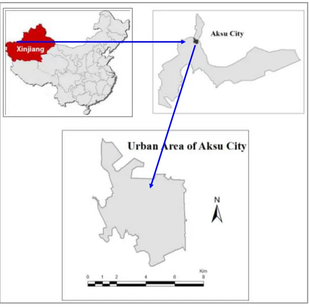
1.4 Study Area ... 4

1.6 Dissertation Organization ... 6

2. LITERATURE REVIEW ... 8

2.1 Urban Heat Island (UHI) ... 8

2.2 Application of Thermal Remote Sensing in Detecting LST ... 9

2.3 Urban Greenspace ... 11

2.4 Integrated Analysis: Urban Greenspace and Land Surface Temperature ... 15

3. RESEARCH METHODOLOGY ... 16

3.1 Data Collection ... 17

3.1.1 Remote Sensing Data ... 17

3.1.2 Reference Data ... 19

3.2 Tools ... 19

3.3 Image Processing ... 20

3.4 Extracting Urban Greenspace ... 21

3.4.1 Landcover classes ... 21

3.4.2 Image classification ... 21

3.4.3 Accuracy Assessment ... 23

3. 5 Landscape Metric Selection and Calculation ... 24

3. 6 Estimating Land Surface Temperature ... 26

3.6.1 Principles of Land Surface extraction ... 26

3.6.2 TM/ETM+ Temperature Extraction Algorithm Overview ... 28

3.6.3 Surface Brightness Temperature Retrieval of the Study Area ... 31

3.6.4 Surface emission rate calculation of the study area ... 32

ix

3.7 Statistical Correlation Measures ... 33

4. RESULTS AND DISCUSSION ... 37

4.1 Urban Greenspace Map ... 38

4.2 Spatial Pattern of Urban Greenspace ... 39

4.3 Land Surface Temperature Map ... 39

4.4 Descriptive Analysis of LST and Urban Greenspace ... 41

4.4 Discussion ... 44

5. CONCLUSIONS ... 47

BIBLIOGRAPHIC REFERENCES... 48

APPENDICES ... 56

Appendix 1: Land Cover Land Use map of Aksu City ... 56

Appendix 2: Part of the Matlab Code ... 57

Appendix 3: Intermediate Results Of Normalized Mutual Information ... 61

x

INDEX OF TABLES

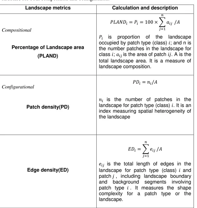
Table1 Common thermal satellite sensors Table2 Description of Landsat image data Table3 The definition of landscape metrics

Table4 Estimate of the average atmospheric temperature table

Table5 Estimation of atmospheric transmittance for Landsat-5 TM Band6 Table6 Values of Lmax and Lmin for reflecting bands of Landsat-5 TM Table7 Value of K₁ and K₂

xi

INDEX OF FIGURES

Fig. 1 Map of the study area

Fig.2 Urban Heat Island Profile showing temperature differences for specific land cover of the urban area.

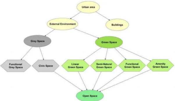
Fig. 3 Structure of urban greenspace

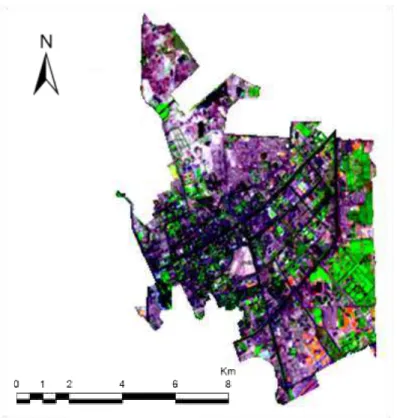
Fig. 4 The flow chart of the research data and methodology Fig. 5 Urban area of Aksu, NW China (5,4,3 bands RGB) Fig. 6 Land cover classes

Fig.7 Urban greenspace map

Fig.8 Grid map of urban greenspace metrics Fig.9 LST map of study area

2

1. INTRODUCTION

1.1 Background of the Study

The urban heat island (UHI) refers to the phenomenon of higher atmospheric and surface temperatures occurring in urban areas than in the surrounding rural areas. The UHI phenomena are widely observed in cities despite their sizes and locations (Tran et al. 2006, Imhoff et al. 2010). Increased temperatures due to UHI may alter species composition and distribution (Niemelä 1999), increase air pollution (Sarrat et al. 2006, Weng and Yang 2006, Lai and Cheng 2009), and affect the comfort of urban dwellers and even lead to greater health risks (Patz et al. 2005). Therefore, since first reported in 1818, UHI has become a major research focus in urban climatology and urban ecology (Arnfield 2003, Weng 2009).

The intensity and spatial pattern of UHI is a function of land surface characteristics (e.g. albedo, emissivity, and thermal inertia), urban layout/street geometry (e.g. canyon height-to-width ratio and sky view factor), weather conditions (e.g. wind and humidity), and human activities(Hamdi and Schayes 2007, Rizwan, Dennis, and Liu 2008a, Taha 1997, Unger 2004, Voogt and Oke 1998). Many of these factors, especially land surface characteristics, are primarily determined by land use/land cover (LULC). For example, vegetation usually has higher evapotranspiration and emissivity than built-up areas, and thus has lower surface temperatures (Hamada and Ohta 2010, Weng, Lu, and Schubring 2004). This suggests that increases in the amount of greenspace can be an effective means to improving the urban thermal environment.

3

focusing on the relationship between LST and greenspace composition. In particular, the significant negative relationship between LST and vegetation abundance was well documented (Voogt and Oke 2003, Weng, Lu, and Schubring 2004, Chen, Zhao, et al. 2006, Tran et al. 2006, Weng 2009). However, less studied is the relationship between LST and configuration of greenspace (Liu and Weng 2008, Weng, Liu, and Lu 2007, Zhao et al. 2011). Some preliminary studies have demonstrated that both air and surface temperatures may be related to the configuration of greenspace(Bowler et al. 2010, Cao et al. 2010, Honjo and Takakura 1991, Yokohari et al. 1997, Zhang et al. 2009). For example, two recent studies showed that the size and shape of a vegetation patch affected its cool island effects, the phenomenon that the temperature of greenspace is lower than its surrounding areas (Cao et al. 2010, Zhang et al. 2009). These studies were conducted at the patch level, only focusing on the size and shape of greenspace, however few have examined the effects of configuration of greenspace on LST at the landscape level(Yokohari et al. 1997, Zhang et al. 2009, Zhou, Huang, and Cadenasso 2011), at which urban greenspace planning and management are usually implemented. Exploring the relationship between LST and spatial pattern, especially configuration of greenspace at the landscape level, can help us better understand the LST–vegetation relationship, and provide insights for urban greenspace planning and management.

1.2 Objectives

The intent of the study is to quantify the urban greenspace and estimate the land surface temperature of the aksu city and analyze the effects of spatial pattern of greenspace on land surface temperature.

Specifically,

 to extract and map the urban greenspcace infromation from the landast TM imagery (image);

 to estimate the land surface temperature of the study, and data will be retrived from Landsat TM thermal band;

4

 to carry out statistical analysis between the urban greenspace patterns and landsurface temprature.

 to provide implication for urban planning and land use management

1.3 Research Questions

This study, taking the oasis city Aksu as case study, tried to answer the following two questions:

 Does spatial pattern, especially configuration of greenspace affect LST ?

 What is the relative importance of composition and configuration of greenspace in explaining the variance of LST?

In this work, the spatial pattern of greenspace refers to the composition (i.e., percent cover) of greenspace, and its spatial distribution or configuration. The spatial pattern of greenspace will be measured by a series of selected landscape metrics that will be discussed in detail in the methodology section. The research questions will be addressed using normalized mutual information measure.

1.4 Study Area

5

Aksu City is situated in the hinterland of the Eurasian continent, rich in light and heat resources. It experiences a long frost-free period, which is around 205 to 219 days. The climate is dry with little rainfall since it is the one of the most remote cities from the ocean, hence rainfall is extremely rare and does not exceed 50 mm per year with average annual evaporation of 1950 mm. The study area is flat. The climatic and the physiographic conditions are mostly constant across the region. Therefore, it is an ideal area to explore the relationship between LST and spatial pattern of greenspace in arid and semi arid land.

6

Fig. 1 map of the study area

1.6 Dissertation Organization

7

8

2. LITERATURE REVIEW

2.1 Urban Heat Island (UHI)

The urban heat island (UHI) refers to the phenomenon of higher atmospheric and surface temperatures occurring in urban areas than in the surrounding rural areas and generally because of changing urban land cover. As a major component of urban climate, UHI has been a concern for more than 40 years(Chen, Yang, et al. 2006). This phenomenon was first discovered in London over 150 years ago by Howard (1833) and has since been studied in many of the largest cities around the world. Heat islands have been documented in most or the major cities in all around the world. Recent decades have seen the study of urban heat islands extended to many smaller and more diverse cities around the world. Over the past few years, UHI has been investigated in cities as diverse as Lódi, Poland(Klysik and Fortuniak 1999), Reykjavik, Iceland (Steinecke 1999), Fairbanks, Alaska (Magee, Curtis, and Wendler 1999), Grnnadn, Spain(Vez, Rodríguez, and Jiménez 2000) and Beijing, China (Lin and Yu 2005)

Fig.2 Urban Heat Island Profile showing temperature differences for specific land cover of the urban area. (Source: Environmental Protection Agency) Source: http://www.urbanheatislands.com/

9

in the central business district(s) or other areas of high urban density. The heat island is mitigated somewhat by areas of vegetation and low urban density, such as golf courses. parks, and playing fields.

2.2 Application of Thermal Remote Sensing in Detecting LST

In past several decades, remote sensing technology has contributed well to the study of urban areas and urban heat islands. One of the earliest applications of spaceborne measurements was for surface temperature and its relationship to the urban heat island effect and urban climate. (Rao 1972)is credited with the first study of urban heat islands from an environmental satellite. Since then, remote sensing has become vital in the field of urban studies, including the study of urban climate and the urban heat island.

10

Another way of assessing temperature simultaneously across a wide surface area and acquiring a synoptic view of a study area is by using remote sensing technology. Airborne and satellite remote sensing platforms offer away of capturing data related to land surface temperature through thermal sensors. Additionally, data in other bands of the spectrum can be used to assess land cover for levels of vegetation and the extent of urbanization through use of measures like the normalized difference vegetation index or NDVI. Satellites in particular offer an efficient mode of data collection, and those in the Landsat program have been collecting data on a world-wide basis since the 1970’s. Satellite data from Landsat, AVHRR, MODIS and the Terra satellite has all been used to study land surface temperature. The Landsat Thematic Mapper, or TM series of satellites has accumulated a particularly extensive archive of images.Landsat 5 has been in operation since March 1984, providing 120 meter spatial resolution images, which is adequate for medium resolution urban temperature studies. Both MODIS and Advanced Very High Resolution Radiometer, or AVHRR satellites collect data in the thermal band, however their low spatial resolution of 1 and 1.1Km per pixel limits suitability for urban studies. Another instrument, Advanced Spaceborne Thermal Emissions & Reflection Radiometer, or ASTER mounted on the TERRA satellite was launched in 1999. It provides higher spatial resolution data, at 90 meter per pixel. Both Landsat and TERRA have 16 dayground coverage cycles.

11

accurate method for measuring LST with a spatial resolution adequate for urban studies. It offers a low-overhead and efficient land surface temperature survey method.

How Urban Heat Islands are sensed?

There are two types of UHIs that are of equal importance for investigation: The Su rface Urban Heat Island (SUHI) and the Atmospheric Urban Heat Island (AUHI ). Both UHIs are interconnected, though one is an effect of the other.

The SUHI is an indirect measurement of surface temperature that has been inve stigated primarily with airborne or satellite thermal infrared sensors. Atmospheri c corrections and temperature calibrations must be made to accurately use this type of measurement. Satellites that carry such sensors include: NOAA AVHRR (Advanced Very High Resolution Radiometer) and Landat TM & ETM+ Band 6 T hermal low and high gain sensors.

The first satellite observation of UHIs was reported by (Rao 1972). The measurements have improved since the early 1970s as the spatial re solution of the satellite sensors has been improved dramatically. For instance, A VHRR has a pixel resolution of 1.1 x 1.1 km and has a very large swath width of ~2000 km, andthus shows a relatively large area at low resolution. Landsat TM’s infrared sensor has a pixel resolution of 120 m and Landsat ETM+ has a resolution of 60 m. The increased resolution of Landsat’s sensor also limits the swath to 185km wide.

2.3 Urban Greenspace

Greenspaces refer to those land uses that are covered with natural or man-made vegetation in the built-up areas and planning areas (Wu 1999).

12

greenspace is by definition “land that consists predominantly of unsealed, permeable, ‘soft’ surfaces such as soil, grass, shrubs and trees … whether or not they are publicly accessible or publicly managed”. (Jim and Chen 2003) suggested that “greenspaces in cities exist mainly as semi-natural areas, managed parks and gardens, supplemented by scattered vegetated pockets associated with roads and incidental locations.” Fig. 3 illustrates one version of the definition of urban green space and the difference between urban green space and other types of urban open space or grey space (land that consists predominantly impermeable surfaces, such as roads, car parks, pavements and town squares etc). In the present study, urban green space is broadly defined as all types of vegetation found in the urban environment, including urban parks and gardens, outdoor playgrounds, open woodland and grassland fields, regardless of their composition and ownership.

Fig. 3 structure of urban greenspace

Significance and Benefits of Urban Greenspace

13

and Chen 2003), moderating urban climate(Weng 2009, Weng, Lu, and Schubring 2004, Landsberg 1981)offering social inclusion and health benefits (Kaplan and Kaplan 1989) , increasing property values (Anderson and Cordell 1988, Luttik 2000), advancing cities’ economic development (Arvanitidis et al. 2009) and improving people’s quality of life(Lo and Faber 1997, WEBER and Hirsch 1992).In short, the significance of urban green space in providing a broad range of benefits and enhancing urban sustainability is profound. Therefore, estimating urban green space patterns and changes is becoming increasingly important in ecologically oriented city planning and environmentally sustainable urban development.

Urban green space plays an important role in supporting urban communities ecologically, economically and socially. When drastic changes occur to urban green space, the environment, economy and quality of human well-being are affected (James et al. 2009). Therefore, a better understanding of urban green space benefits is crucial for implementing better urban planning strategies.

14

Second, urban green space has economic values. (Anderson and Cordell 1988) provide empirical evidence that trees are associated with increase in residential property values. (Luttik 2000) suggests housing price may be used as a guiding principle to quantify the socio-economic value of ecological factors. It has been demonstrated that the distribution of urban green space can influence the real estate market. (Bolitzer and Netusil 2000)show that proximity to an open space, such as public parks, natural areas and golf courses, and the type of open-space can increase the sale price of homes. They conclude that both distance from a home to an open space and the type of open space have significant effects on the housing market. These studies show that houses located in a comfortable living environment with attractive settings and pleasant views can have an added value over similar, less favourably located houses. Therefore, urban green space increases property values and affects the housing market (housing prices and housing values) positively.

15

2.4 Integrated Analysis: Urban Greenspace and Land Surface

Temperature

16

3. RESEARCH METHODOLOGY

This section describes the data and methods that were applied in data acquisition, pre-processing (geo-reference and geometric correction), pre-processing, presentation and analysis data with a view to achieve the designed objectives and the research questions posed. This allowed us analysis of change and to draw conclusions about effects of spatial pattern of greenspace on land surface temperature. Fig. 4 depicts the flow chart how the research data, methods and analysis were organized in a brief way.

17

3.1 Data Collection

3.1.1 Remote Sensing Data

Currently remote sensing data for detecting land surface thermal environment generally include sixth band of Landsat TM and Landsat ETM+, fourth and fifth bands of AVHRR on NOAA meteorological satellite, 31st and 32nd bands of MODIS satellite, 10th , 11th , 12th ,13th and 14th bands of ASTER the satellite. The spatial resolution of MODIS data vary from 250m to 1000m, but spectral resolution is relatively high. The spatial resolution of AVHRR data is 1000m. ASTER thermal infrared band has 90m of spatial resolution. Landsat TM and ETM+ thermal infrared bands are featured with spatial resolution of 120m and 60m (Table1). In order to maintain the consistency of data radiation characteristics as well as to investigate the detailed thermal structure of land surface more effectively, Landsat images were chosen as the data source of the research (Fig.5). Table2 describes the related information of the Landsat 5 images used for further processing.

18 Satellite Sensor Attribution

Number of TIR band numbers spectral range of TIR (µm) spatial resolution

NOAA AVHRR the United

States 2

3.55-3.93

10.3-12.5

1.1km-8km

ERS ATSR ESA 3

Central

wavelength

3.7, 11, 12 1km

Terra&Aqua MODIS America 16

3.66-14.385 1km

RESURS-1 MSU-SK Russia 1 10.4-12.6 600m

BIRD HSRS Germany 2

3.4-4.2

8.5-9.3

370m

CEBER IMRSS China, Brazil 1 10.4-12.5 156m

Landsat-5 TM the United

States 1 10.4-12.5 120m

Terra&Aqua ASTER Japan,

America 5

8.125-11.65 90m

Landsat-7 ETM+ the United

States 1 10.4-12.5 60m

Table1. Common thermal satellite sensors

Satellite Sensor Data Acquisition date Resolution(m) visible/thermal

Product

Quality

Landsat 5 TM/MSS 19 August, 2011 30/120 good

19

Landsat 5 path 147, row 31 covers the whole study area. The map projection for collected satellite images is Universal Transverse Mercator(UTM) within 44 North. Datum is World Geodetic System (WGS) 84(USGS 2010).

3.1.2 Reference Data

In this study, it was necessary to employ a variety of methods to develop reference data sets for training samples and accuracy assessment. It is also apparent that ancillary data such as high resolution imageries and existing map of the study area were essential for extracting and assessing the accuracy of the urban greenspace map. The study mainly relied on the land use map of Aksu city with a scale of 1:150000 (produced by Land Resources Bureau of Aksu City and Department of Resource and Environmental Science, Xinjiang University, China. Published on Jun. 2012) as reference for urban greenspace mapping and its accuracy assessment. Google Earth was another option to get some ideas about detecting urban greenspace pattern of Aksu city. In conclusion these were the reference data used for training site selection and preparing the urban greenspace map.

The referenced land use map of Aksu city is attached in Appendix.

3.2 Tools

20

representations were used to present describe and analyze the outcomes of the study and write up the whole report.

3.3 Image Processing

21

3.4 Extracting Urban Greenspace

3.4.1 Landcover classes

Fig.6 shows the classification land cover class system established for this study. The land cover classes applied in this paper are adopted from the classification used by Chinese Environment Agency, which describes land cover (and partly land use) according to a nomenclature of 38 classes organized hierarchically in different levels. This system is used for pixel-based image classifications. The entire image is classified into four classes, namely urban greenspace, residential area, construction site and water body. The ultimate goal of image classification is to extract urban greenspace information in order to further investigate its relationship with land surface temperature.

Fig.6 Landcover classes

3.4.2 Image classification

Urban greenspace is an important symbol of evaluating urban civilization and modernization(DU and GAO 2000). As the natural productivity, green space plays important roles in urban ecological systems. Compared with the traditional surveying method and the mathematical or statistical analysis, green space information extraction from remote sensing images has noticeable advantages: (1) intelligent and shorter time requirement; (2) smaller human impact and higher accuracy; and (3) higher visualization, facilitate comprehensive evaluation. To take use of these

Study Area

Urban Greenspace

ResidentialArea

Construction Site

22

advantages, image classification method was used to extract the urban greenspace information(Huapeng et al. 2007).

In remote sensing, there are different image classification techniques. Their appropriateness depends on the purpose of landcover maps produced for and the analyst’s knowledge of the algorithms he/she is using. Classification methods can also be viewed as pixel-based, object-oriented, fuzzy classification, etc. Selection of appropriate classification methods and efficient use of multisource remotely sensed data are useful for minimizing the classification errors and improve the accuracy (Lu and Weng 2007). Regarding mentioned points above, for this study, pixel-based supervised image classification was applied.

Pixel-based Supervised Image Classification

A pixel-based supervised image classification is based on the theory that it uses pixels in the training samples to develop appropriate discriminant functions to distinguish each class. The data vectors typically consist of a pixel’s grey level values from multi-spectral channels (Shackelford and Davis 2003). Training samples are needed to train the classifier based on prior knowledge of the study area features. This knowledge is obtained through ground truth and familiarity with associated ancillary maps and images. Then the statistical analysis is performed on the multiband data for each class. All pixels in the images outside the training sites were then compared with the class discriminants and assigned to the class they are closest to or remained unclassified (Navulur 2006). To conclude, the four stages involved in a supervised classification are: (1) class definition, (2) pre-processing, (3) training and (4) automated pixel assignment. In this study, pixel-based supervised maximum likelihood image classification is performed in ENVI 4.1.

23

classification map and land cover map were used to create ground control signatures. The image was classified into four major landcover classes and they include urban greenspace, residential areas, construction site and water bodies.

3.4.3 Accuracy Assessment

Assessment of classification accuracy is critical for a map generated from any remote sensing data. Although accuracy assessment is important for traditional remote sensing techniques, with the advent of more advanced digital satellite remote sensing the necessity of performing an accuracy assessment has received new interest (Congalton 1991). Currently, accuracy assessment isconsidered as an integral part of any image classification. This is because image classification using different classification methods or algorithms may classify or assign some pixels or group of pixels to wrong classes. In order to wisely use the landcover maps which are derived from remote sensing and the accompanying land resource statistics, the errors must be quantitatively explained in terms of classification accuracy. The most common types of error that occurs in image classifications are omission or commission errors.

The widely used method to represent classification accuracy is in the form of an Error Matrix sometimes referred as Confusion Matrix. Using Error Matrix to represent accuracy is recommended and adopted as the standard reporting convention (Congalton 1991). It presents the relationship between the classes in the classified and reference maps. The technique provides some statistical and analytical approaches to explain the accuracy of the classification. In this study, overall, producer’s and user’s accuracy were considered for analysis. Kappa Coefficient, which is one of the most popular measures in addressing the difference between the actual agreement and change agreement, was also calculated. The kappa is a discrete multivariate’s technique used in accuracy assessment (Fan, Weng, and Wang 2007). The Kappa coefficient is calculated according to the formula given by (Congalton 1991):

24 r = the number of rows in the error matrix

= the number of observations in row i column i(along the diagonal) = is the marginal total of rowi(right of the matrix)

= the marginal total of column i(bottom of the matrix) = the total number of observations included in the matrix

The reference data used for accuracy assessment are usually obtained from aerial photographs, high resolution images (e.g. IKONOS and QUICKBIRD), and field observations. In this study, the assessment was carried out using Google Earth and existing landcover maps as a reference. A set of reference points has to be generated ; thus, three hundred (300) randomly allocated training points were generated for accuracy assessment. These points were verified and labeled against reference data. Error matrices were designed to assess the quality of the classification accuracy of the newly generated landcover map. The error matrix can then be used as a starting point for a series of descriptive and analytical statistical techniques (Congalton 1991). Overall accuracy, user’s and producer’s accuracies, and the Kappa statistic were then derived from the error matrices.

3. 5 Landscape Metric Selection and Calculation

25

types within the landscape, without explicitly describing its spatial features (i.e., percentage land of a certain cover). Landscape configuration metrics measure the spatial distribution of patches within the landscape (i.e., degree of aggregation and contagion) (Alberti 2005). Three commonly used landscape metrics were selected to relate land surface temperature with spatial pattern of urban greenspace according the following principles (Riitters et al. 1995, Li and Wu 2004, Lee et al. 2009, Riva-Murray et al. 2010): (1) important in both theory and practice, (2) easily calculated, (3) interpretable, and (4) minimal redundancy. Table 3(for detailed calculation equation and comments, see McGarigal et al. 2002) shows the three landscape metrics. They are selected to provide complementary information about landscape structure for both composition and configuration.

Landscape metrics Calculation and description

Compositional

Percentage of Landscape area

(PLAND)

is proportion of the landscape occupied by patch type (class) ; and n is the number patches in the landscape for class ; is the area of patch . A is the total landscape area. It is a measure of landscape composition.

Configurational

Patch density(PD)

is the number of patches in the landscape for patch type (class) . It is an index measuring spatial heterogeneity of the landscape

Edge density(ED)

is the total length of edges in the

landscape for patch type (class) and patch , including landscape boundary and background segments involving patch type . It measures the shape complexity for a patch type or the landscape.

26

With FRAGSATS software we can have the option of conducting a local structure gradient or moving window analysis and outputting the results as a new grid for each selected metric. If we select a moving window analysis, then we must specify the level of heterogeneity (class or landscape) and the shape (round, square or hexagon) and size (radius or length of side, in meters) of the window to be used. A window of the specified shape and size is passed over every positively valued cell in the grid (i.e., all cells inside the landscape of interest). However, only cells in which the entire window is contained within the landscape are evaluated. Within each window, each selected metric at the class or landscape level is computed and the value returned to the focal (center) cell. The moving window is passed over the grid until every positively valued cell containing a full window is assessed in this manner.

In our case, we used 8-cell rule and 500m-radius circular window was used. The window moves over the 1andscape one cell at a time, calculating the selected metric

within the window and returning that value to the center cell and output a new grid file for each selected file metric.

3. 6 Estimating Land Surface Temperature

3.6.1 Principles of Land Surface extraction

The nature of material is to continuously radiate electromagnetic waves with certain energy and spectral distribution, as long as the temperature is more than absolute zero (273.15K). Moreover, the intensity and the features of spectral distribution of radiant energy are function of material type and temperature. In atmospheric transmission process, thermal infrared passes through the two windows (3-5m and 8-14m).

27

characteristics of the surface and the sun is the basis of the thermal infrared remote sensing. Generally speaking, the object of the radiation energy budget is uneven, so the temperature of the object is unstable. But at a specific moment, the state of the object can be considered as balanced. Thus, we are allowed to use certain temperature to characterize and analyze the radiation energy of an object. The following content describes the basic thermal radiation law of objects.

(1) Kirchhoff’s Law

Kirchhoff found that at the same temperature, for various objects, ratio between the emitted energy W and the absorption rate within per unit time and per unit area is a constant. This ratio has nothing to do with the nature of the object itself; it is equal to the black body radiation energy WB of same area under the same temperature condition. Its mathematical expression is following:

W /= WB

Can also be written as: = W / WB

From previous formula  = W/WB, so   equal to the absorption rate and emissivity of the object. (If an object does not absorb electromagnetic radiation at certain wavelength, it will not transmit the same wavelength of electromagnetic waves)1

(2) Stephen (Stefen) - Boltzmann

The law has proved that the total radiant heat energy emitted from a surface is proportional to the fourth power of its absolute temperature.

The law applies only to blackbodies, theoretical surfaces that absorb all incident heat radiation. For general objects the law needs to be amended. The emitted thermal radiation energy of objects, according to Kirchhoff and Stephen (Stefen) - Boltzmann's law2, equals to,

4 T

W   is Emission rate,

1

28

Or W T4  is absorption rate.

The formulas above show that the thermal radiation energy of general objects is proportional to the fourth power of its absolute temperature and its emission rate. Hence, if there is a slight difference in object temperature, it will cause more significant change. As long as the emission rate of surface features is different, two objects with the same temperature will exhibit different radiation characteristics. Thus the object heat radiation characteristics form the theoretical basis of the thermal infrared remote sensing.

3.6.2 TM/ETM+ Temperature Extraction Algorithm Overview

Currently there are three types of land surface temperature retrieval algorithms for TM/ETM+ images, which are radiation conduction equation method, mono-window algorithm and single-channel algorithm(DING Feng 2006). Radiation conduction equation method requires real-time atmospheric profile data but acquisition of this type of data is rather difficult; Parameters of mono-window algorithm need near-surface temperature, and atmospheric water content; the only required atmospheric parameters for single-channel algorithm is moisture content of atmosphere. The algorithms are outlined below:

(1) Radiation Conduction Equation

This method is also known as atmospheric correction method. The basic idea is to first estimate the impact of the atmosphere on surface thermal radiation, specifically the atmospheric sounding profile data is measured by synchronous satellite transit or MODTRAN, ATCOR, 6S atmospheric model; then this atmospheric effects will be subtracted from total thermal radiation observed by satellite sensor. The is the process of obtaining the surface thermal radiation intensity. At the end this intensity is converted to the corresponding surface temperature. The algorithm expression:

  



 _{S atm atm}

sensor BT I I

29

Where Isensor is intensity of surface emissive radiation measured by sensor;  is

surface emission rate; B

 

Plank's law where

 



atm

I and I_atm are

atmospheric thermal downstream and upstream radiation intensity respectively;  is atmospheric transmittance. 

atm

I and I_atm can be calculated by using real-time

atmospheric sounding profile data or 6S atmospheric modeling software. Therefore, as long as surface emissivity is measured, the B

 

formula described above. To further calculation following formula will be used to retrieve the land surface temperature:

 





S K K BT

T  ₂/ln1 ₁/

Where TS is surface temperature (Kelvin); for Landsat TM K1andK2 are constants

1

K =607.76





2

K =1260.56





Radiation conduction equation method limits the algorithm for practical application due to the lack of real-time atmospheric profile data.

(2) Single-Channel Algorithm

Single-channel algorithm only relies on one thermal infrared band to invert the land surface temperature, The formula:





     

 ( ₁ SENSOR ₂)/ ₃

S L

T

Where TS is land surface temperature (K); Lsensor is radiation intensity measured by

sensor (unit: _ 2_ 1_ 1

m sr m

W  );  land surface emission rate;  , ,₁,₂,₃are

intermediate variables and explained by formulas below:









 1/ / 2 * 4 / ₁ 1/

2 

30 1234 . 1 15583 . 0 14714 . 0 2

1  

 w w

5294 . 0 37607 . 0 1836 . 1 2

2   

 w w

39071 . 0 8719 . 1 04554 . 0 2

3   

 w w

Where C1 and C2 are constants of PLANK function.

1

c = 1.19104 * 108Wm4 m2sr1

c₂= 14387.7mk

SENSOR

T is pixel brightness temperature detected by sensor (Kelvin);  is effective role

wavelength; w is The total water vapor content of atmospheric profiles. (gcm2).

(3) mono-window algorithm

Mono-window algorithm, invented by (Zhi-hao, Zhang, and Karnieli 2001). It is a derivation of land surface thermal radiation conduction equation. By using this method land surface temperature can be extracted from TM sixth band. The calculation procedure is explained as following:

















T_S  1   1     ₆ _a /

Where TSis land surface temperature (Kelvin); a and b are variables, respectively

-67.355351, 0.458606; C and D are intermediate variables. C =  , D =



 







31

Atmosphere type Estimating equation

Average atmosphere of America 1976 Ta 25.93960.88045T0

Average tropical atmosphere

(North latitude15º, annual average ) Ta 17.97690.91715T0 Mid-latitude summer average atmosphere

(North latitude 45º, July) Ta 16.0110.92621T0 Mid-latitude winter average atmosphere

(North latitude 45º , January) Ta 19.27040.91118T0

Table 4. Estimate of the average atmospheric temperature table

atmospheric profile

Moisture content





/cm g w

Estimating equations of

Atmospheric

transmittance

High temperature (35Cº)

0.4-1.6 T=0.97429-0.08007w

1.6-3.0 T=1.031412-0.11536w

low temperature (18 Cº) 0.4-1.6 T=0.982007-0.09611w 1.6-3.0 T=1.05371-0.14142w

Table 5. Estimation of atmospheric transmittance for Landsat TM Band6

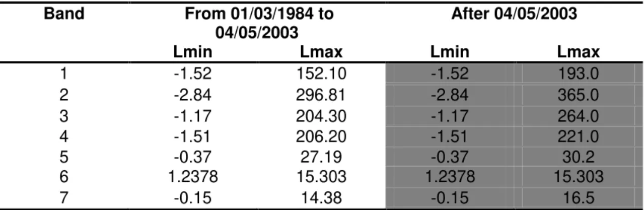
Band From 01/03/1984 to 04/05/2003

After 04/05/2003

Lmin Lmax Lmin Lmax

1 -1.52 152.10 -1.52 193.0

2 -2.84 296.81 -2.84 365.0

3 -1.17 204.30 -1.17 264.0

4 -1.51 206.20 -1.51 221.0

5 -0.37 27.19 -0.37 30.2

6 1.2378 15.303 1.2378 15.303

7 -0.15 14.38 -0.15 16.5

Table 6. Values of Lmax and Lmin for reflecting bands of Landsat-5 TM (W˙m-2-sr-1˙μm-1)

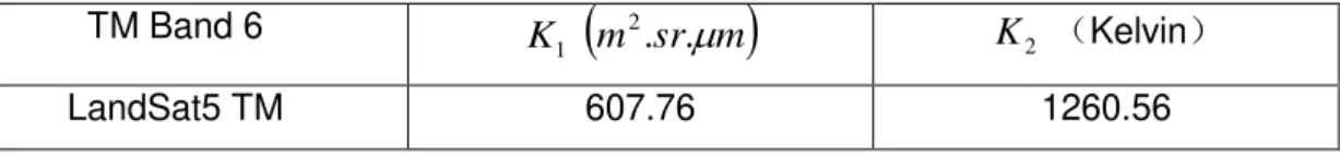
3.6.3 Surface Brightness Temperature Retrieval of the Study Area

32





K

T₆  ₂/ln1 ₁/

Where T₆ is brightness temperature of the study area; K₁ and K₂ is default

pre-launch constants (Table 7), L_is radiance of sixth band calculated.

TM Band 6

1

K





LandSat5 TM 607.76 1260.56

Table 7 Value of K₁ and K₂

3.6.4 Surface emission rate calculation of the study area

Surface emissivity is an important element to calculate the land surface temperature . Surface emissivity has considerable effect on accuracy of land surface temperature extraction and the important sources of error. The study shows that the relative error of 0.01 in emission rate can cause error of 0.75K in land surface temperature. Consequently, the resulting error towards extraction accuracy is much more bigger than the error that atmosphere causes. Therefore, people have been greatly concerned about acquisition of surface emissivity information in many ways, such as laboratory, field and space measurements.

In this paper given emissivity of soil and vegetation as precondition, the weighted hybrid model , which proposed by Sobrino and based on land cover types, was used and the surface emissivity was calculated by NDVI classification. The formula as follows: ε=            5 . 0 99 . 0 5 . 0 2 . 0 ) 1 ( 2 . 0 97 . 0 NDVI NDVI P P NDVI V S V V  

Where ε is the surface emissivity, εv vegetation emissivity, εsbare soil emissivity εv =0.99, εs = 0.97, pv vegetation coverage.

33 Pv=

)

( _{max min}

min

NDVI NDVI

NDVI NDVI

 

NDVI is vegetation index of a pixel. NDVImin and NDVImax are minimum and maximum NDVI values of the study area. In fact, the vegetation cover and leaf area index (LAI) change over time and space. Healthy vegetation has higher humidity value. For all soil background, if green vegetation coverage increases with increasing humidity values. This phenomenon is particularly evident when it comes to dry soil, namely NDVImin = 0.2, NDVImax = 0.5.

3.6.5 Land surface temperature calculation of the study area

This paper used mono-window algorithm, proposed by Zhihao, to calculate land surface temperature. The average atmospheric temperature was obtained from the formula displayed on Table 4 (grayed area); atmospheric transmittance was estimated based on formula showed on Table5 (grayed area). According to s previously calculated brightness temperature and surface emissivity, real temperature map of study area was produced with mono-window algorithm.

3.7 Statistical Correlation Measures

Some previous studies have already showed us about the negative correlation between the land surface temperature and urban green space. However, the studies which can indicate us how the spatial pattern of greenspace effects the landsurface temperature are significantly rare. To fill this gap, this study applied statistical correlation methods to further reveal the spatial relationships between the land surface temperature and spatial pattern of urban greenspace.

In information theory, we can find information measures that can quantify how much a given random variable can predict another one3. In this respect, the normalized

34

mutual information measure was applied to figure out the correlation between the land surface temperature and spatial pattern or urban greenspace.

Not only is mutual information widely used as a criterion for measuring the degree of independence between random variables but it also measures how much a certain variable can explain the information content about another variable, being a generalized correlation measure. Thus, special relationships between spatial pattern of urban greenspace and land surface temperature (random variables) can be defined based on this measure as a relevance criterion.

In following section some important concepts and properties in information theory will be introduced.

Entropy

In information theory, entropy is a measure of the uncertainty in a random variable. In this context the term usually refers to the Shannon entropy, which quantifies the expected value of the information contained in a message4. The Shannon entropy of a random variable X with probability density function for all possible events

is defined as

In the case of discrete random variable X, entropy H(X) is expressed as

Where represents the mass probability of an event from a finite set of possible values. Entropy is often taken as related amount of information of a random variable.

35 Mutual information

In probability theory and information theory, the mutual information (sometimes known by the archaic term trans-information) of two random variables is a quantity that measures the mutual dependence of the two random variables.

Formally, the mutual information of two discrete random variables X and Y can be defined as:

where p(x,y) is the joint probability distribution function of X and Y,

and and are the marginal probability distribution functions of X and Y respectively.

I is always a nonnegative quantity for two random variables, being zero when the

variables are statistically independent. The higher the I, the higher the dependence

between the variables. Furthermore, the following property about two random vari-ables always holds:

Mutual information I can be expressed in terms of entropy measures according to the

following expression:

36 Normalized mutual information measure

So far, I has been introduced as an absolute measure of common information shared

between two random variables. However, as we can infer from (5), I by itself would

not be suitable as a similarity measure. The reason is that it can be low because either the variables present a weak relation (such as it should be desirable) or the entropies of these variables are small (in such a case, the variables contribute with little information). Thus, it is convenient to define a proper measure, so that it works independently from the marginal entropies and also measures the statistical dependence as a similarity measure .

Thus, the normalized mutual information measure will be used to assess the dependencies between the variables. In fact there exit numerous definitions of information-based criteria in applications among them, one important expression is the normalized mutual information measure defined as

This expression presents another type of “correlation measure and sometimes is called as “asymmetric dependency coefficient (ADC)”. However, tow definitions in (number 6) will produce unequal values due to their asymmetric property in the definitions. Therefore, normalized mutual information was proposed with symmetric property, such as

In this study, the expression (6) was applied to measure the normalized mutual information between the different variables since the focus of the work is to find out the correlation between the land surface temperature, which is chosen as reference of target variable , and other variables including PLAND, ED and PD.

37

38

4. RESULTS AND DISCUSSION

4.1 Urban Greenspace Map

Urban greenspace was mapped using remote sensing classification techniques (Fig.7). In order to achieve the best classification outcome to evaluate the classification results, confusion/error matrices were used. It is the most commonly employed approach for evaluating per-pixel classification (Lu and Weng 2007). The accuracy was assessed with cross-validation against landcover map and Google Earth Imageries. Using these reference data and the classified maps, confusion matrices were constructed. The resulting Landsat land use/cover map had an overall map accuracy of 87.6 %. This was reasonably good overall accuracy and accepted for the subsequent analysis and change detection. User’s accuracy of individual classes ranged from 75% to 100 % and producer’s accuracy ranged from 73 % to 100%.

Fig.7 Urban greenspace map

0 1 2 4 6 8

Km

39

Kappa statistics/index was computed for classified map to measure the accuracy of the results. The resulting classification of Landsat land use/cover map had a Kappa statistics of 84.4%. The Kappa coefficient expresses the proportionate reduction in error generated by a classification process compared with the error of a completely random classification. Kappa accounts for all elements of the confusion matrix and excludes the agreement that occurs by chance. Consequently, it provides a more rigorous assessment of classification accuracy.

4.2 Spatial Pattern of Urban Greenspace

To carry out the quantitative analysis of the relationship between the LST and urban greenspace, just having an urban greenspace map or a landcover map is not sufficient. Therefore, as described in methodology section, the compositional and configurational pattern of urban greenspace were calculated. For compositional feature PLAND, for configurational feature PD and ED were chosen and grid map of the landscape metrics were produced (Fig.8).

(a)Percent cover of greenspace (b)Patch density (c) Edge density

Fig.8 Grid map of urban greenspace metrics

4.3 Land Surface Temperature Map

The digital remote sensing method provides not only a measure of the magnitude of surface temperatures of the entire study area, but also the spatial extent of the surface

40

41

Fig.9 LST map of study area

4.4 Descriptive Analysis of LST and Urban Greenspace

Scatter plots (Fig.10) were made to show the relationships between the LST and landscape metrics. The every pixel value of LST map and corresponding values of urban greenspace landscape metrics were used as input data.

0 1 2 4 6 8

Km

42

Fig.10 Scatter plot of LST with PLAND, PD and ED

Considering correlation between the variables, there is a significant, negative linear relationship between LST and all three urban greenspace landscape metrics (Table 8).

A statistically significant, negative linear relationship was shown for PLAND (r = -0.558828). Besides, other two landscape metrics indicated negative relationship

with LST as well. However, PD indicates the weakest negative relationship (r = -0.24852) with LST compare to PLAND and ED (r=-0.49288).

PLAND PD ED

LST -0.55828 -0.24852 -0.49288

Table 8. Correlation coefficients

So as to answer the research questions, the new statistical approach was performed to quantify the relationship between the LST and spatial pattern of urban greenspace. The focus of this section mainly on normalized mutual information analysis since it is more appropriate method to measure the dependencies between different variables.

y = -2.8311x + 889.06 R² = 0.3055

0 20 40 60 80 100

290 300 310 320 330

P LAN D ( %) LST (Kelvin)

y = -0.4772x + 156.99 R² = 0.0539

0 10 20 30 40

290 300 310 320 330

P D ( n/k m 2) LST (Kelvin)

y = -3.3634x + 1077.5 R² = 0.2329

0 20 40 60 80 100

290 300 310 320 330

43

Nevertheless, the outcome of mutual information measure was omitted here considered as an intermediate result of normalized mutual information analysis (attached in appendices).

First of all the normalized mutual information between the LST and single landscape metrics were calculated in order to figure out how the only composition or configuration of greenspace affects the LST. Results are shown below :

= I(PLAND; LST)/H(LST) = 0.7100 =I(PD; LST)/H(LST) = 0.6985

=I(ED; LST)/H(LST) = 0.7033

In next step, to measure the impact of combination of compositional and configurational urban greenspace, joint variables of urban greenspace landscape metrics were formed and normalized mutual information was calculated, such as:

=I(PLAND, PD; LST)/H(LST) = 0.7679 =I(PLAND, ED; LST)/H(LST) = 0.7650 =I(PD, ED; LST)/H(LST) = 0.7832

Finally, all three landscape metrics of urban greenspace were joined into one variable and dependency between this variable and LST was measured.

=I(PLAND, PD, ED; LST)/H(LST) = 0.8694

44

patterns, all types of joint greenspace patterns have more strong effect on LST than the both single compositional and configurational greenspace patterns. The joint effect of (PLAND, PD) has less effect on LST than (PLAND, ED) does. However, the joint

effect of (ED, PD) has relatively higher effect than pervious joint greenspace patterns.

Finally, The strongest effect of greenspace on LST was expressed by three joint landspcape metrics.

4.4 Discussion

Urban greenspace can potentially mitigate the UHI effects, and numerous studies have shown that increases in PLAND can significantly decrease LST(Weng, Lu, and Schubring 2004, Buyantuyev and Wu 2010) Fewer studies, however, have investigated the effects of configuration of greenspace on LST(Yokohari et al. 1997, Zhang et al. 2009, Zhou, Huang, and Cadenasso 2011). Taking the urban area oasis city Aksu as an example, we quantitatively demonstrated that the spatial pattern of greenspace, both the composition and configuration, significantly affected LST.

45

Concerning the configurational metrics, the PD and ED are less correlated with LST than PLAND is. The normalized mutual information analysis also showed that there were less dependences between the LST with individual PD and ED, which is still smaller than the dependence between the PLAND and LST. This means the increase of patch density leads to decrease in mean patch size resulting in a general increase in total patch edges. Therefore, the effects of the increase of patch density on LST were due to the joint effects of a decrease in mean patch size and increase in patch edges on LST. The decrease in mean patch size may increase LST because a larger, continuous greenspace produces stronger cool island effects than that of several small pieces of greenspace whose total area equals the continuous piece(Yokohari et al. 1997, Zhang et al. 2009, Cao et al. 2010). However, the increase of total patch edges may enhance energy flow and exchange between greenspace and its surrounding areas, and provide more shade for surrounding surfaces, which lead to the decrease of LST (Zhou, Huang, and Cadenasso 2011).

The composition of greenspace was more important than the configuration of greenspace in predicting LST, which is consistent with previous findings (Zhou, Huang, and Cadenasso 2011). However, our results also showed that the unique effects of the composition were slightly higher than that of the configuration, and much of the variance of LST was jointly explained because the composition and configuration of greenspace are highly interrelated.

46

urbanizing areas, where available land area for increased greenspace cover is usually very limited (Zhou, Huang, and Cadenasso 2011)(Zhou et al.2011).

47

5. CONCLUSIONS

Taking the urban area of oasis city Aksu area as an example, this study quantitatively examined the effects of spatial pattern of greenspace on LST. it was found that both composition and configuration of greenspace affected LST. The majority of the temperature variance can be attributed to the joint effects of composition and configuration. The unique effects of configuration were only slightly lower than that of composition. Results from this study extend previous findings on the effects of greenspace on UHI and provide insights for effective urban greenspace planning and management.

48

BIBLIOGRAPHIC REFERENCES

Akbari, H., M. Pomerantz, and H. Taha. 2001. "Cool surfaces and shade trees to reduce energy use and improve air quality in urban areas." Solar energy no. 70

(3):295-310.

Alberti, M. 2005. "The effects of urban patterns on ecosystem function." International regional science review no. 28 (2):168-192.

Anderson, L.M., and H.K. Cordell. 1988. "Influence of trees on residential property values in Athens, Georgia (USA): a survey based on actual sales prices." Landscape and Urban Planning no. 15 (1):153-164.

Arnfield, A.J. 2003. "Two decades of urban climate research: a review of turbulence, exchanges of energy and water, and the urban heat island." International Journal of Climatology no. 23 (1):1-26.

Arvanitidis, P.A., K. Lalenis, G. Petrakos, and Y. Psycharis. 2009. "Economic aspects of urban green space: a survey of perceptions and attitudes." International journal of environmental technology and management no. 11 (1):143-168.

Barbosa, O., J.A. Tratalos, P.R. Armsworth, R.G. Davies, R.A. Fuller, P. Johnson, and K.J. Gaston. 2007. "Who benefits from access to green space? A case study from Sheffield, UK." Landscape and Urban Planning no. 83 (2):187-195.

Bolitzer, B., and N.R. Netusil. 2000. "The impact of open spaces on property values in Portland, Oregon." Journal of Environmental Management no. 59 (3):185-193.

Bolund, P., and S. Hunhammar. 1999. "Ecosystem services in urban areas."

Ecological economics no. 29 (2):293-301.

Bowler, D.E., L. Buyung-Ali, T.M. Knight, and A.S. Pullin. 2010. "Urban greening to cool towns and cities: A systematic review of the empirical evidence." Landscape and Urban Planning no. 97 (3):147-155.

Buyantuyev, A., and J. Wu. 2010. "Urban heat islands and landscape heterogeneity: linking spatiotemporal variations in surface temperatures to land-cover and

socioeconomic patterns." Landscape ecology no. 25 (1):17-33.

Cao, X., A. Onishi, J. Chen, and H. Imura. 2010. "Quantifying the cool island intensity of urban parks using ASTER and IKONOS data." Landscape and Urban Planning no. 96 (4):224-231.

Carlson, TN, JA Augustine, and FE Boland. 1977. "Potential application of satellite temperature measurements in the analysis of land use over urban areas." Bulletin of the American Meteorological Society no. 58 (12):1301-1303.

49

of Quantitative Spectroscopy and Radiative Transfer no. 100 (1–3):91-102. doi:

http://dx.doi.org/10.1016/j.jqsrt.2005.11.029.

Chen, X.L., H.M. Zhao, P.X. Li, and Z.Y. Yin. 2006. "Remote sensing image-based analysis of the relationship between urban heat island and land use/cover changes."

Remote Sensing of Environment no. 104 (2):133-146.

Congalton, R.G. 1991. "A review of assessing the accuracy of classifications of remotely sensed data." Remote sensing of Environment no. 37 (1):35-46.

DING Feng, XU Hanqiu. 2006. "Comparisonof Two New Algorithmsfor Retrieving LandSurface TemperaturefromLandsat TMThermal Band." Geo-information Science

no. 8 (3):125-130.

Donovan, G.H., and D.T. Butry. 2009. "The value of shade: estimating the effect of urban trees on summertime electricity use." Energy and Buildings no. 41 (6):662-668. DU, P., and J. GAO. 2000. "Study of Urban Environmental Monitoring and

Management System with 3S Techniques [J]." THE ADMINISTRATION AND

TECHNIQUE OF ENVIRONMENTAL MONITORING no. 2:008.

Fan, F., Q. Weng, and Y. Wang. 2007. "Land use and land cover change in Guangzhou, China, from 1998 to 2003, based on Landsat TM/ETM+ imagery."

Sensors no. 7 (7):1323-1342.

Feist, Blake E, E Ashley Steel, David W Jensen, and Damon ND Sather. 2010. "Does the scale of our observational window affect our conclusions about correlations between endangered salmon populations and their habitat?" Landscape ecology no. 25

(5):727-743.

Gallo, K.P., and T.W. Owen. 1999. "Satellite-based adjustments for the urban heat island temperature bias." Journal of Applied Meteorology no. 38 (6):806-813.

Gallo, KP, AL McNab, TR Karl, JF Brown, JJ Hood, and JD Tarpley. 1993. "The use of NOAA AVHRR data for assessment of the urban heat island effect." Center for Advanced Land Management Information Technologies--Publications:1.

Germann-Chiari, C., and K. Seeland. 2004. "Are urban green spaces optimally distributed to act as places for social integration? Results of a geographical

information system (GIS) approach for urban forestry research." Forest Policy and Economics no. 6 (1):3-13.

Gill, SE, JF Handley, AR Ennos, and S. Pauleit. 2007. "Adapting cities for climate change: the role of the green infrastructure." Built environment no. 33 (1):115-133.

Gregory, D., R. Johnston, G. Pratt, M. Watts, and S. Whatmore. 2009. The dictionary of human geography: Wiley-Blackwell.