www.hydrol-earth-syst-sci.net/16/2285/2012/ doi:10.5194/hess-16-2285-2012
© Author(s) 2012. CC Attribution 3.0 License.
Earth System
Sciences
Interannual hydroclimatic variability and its influence on winter
nutrient loadings over the Southeast United States
J. Oh and A. Sankarasubramanian
Department of Civil, Construction and Environmental Engineering, North Carolina State University, Raleigh, NC 27695-5908, USA
Correspondence to:A. Sankarasubramanian (sankar [email protected])
Received: 17 November 2011 – Published in Hydrol. Earth Syst. Sci. Discuss.: 12 December 2011 Revised: 15 May 2012 – Accepted: 27 June 2012 – Published: 24 July 2012
Abstract.It is well established in the hydroclimatic literature that the interannual variability in seasonal streamflow could be partially explained using climatic precursors such as trop-ical sea surface temperature (SST) conditions. Similarly, it is widely known that streamflow is the most important predic-tor in estimating nutrient loadings and the associated con-centration. The intent of this study is to bridge these two findings so that nutrient loadings could be predicted using season-ahead climate forecasts forced with forecasted SSTs. By selecting 18 relatively undeveloped basins in the South-east US (SEUS), we relate winter (January-February-March, JFM) precipitation forecasts that influence the JFM stream-flow over the basin to develop winter forecasts of nutrient loadings. For this purpose, we consider two different types of low-dimensional statistical models to predict 3-month ahead nutrient loadings based on retrospective climate forecasts. Split sample validation of the predictive models shows that 18–45 % of interannual variability in observed winter nu-trient loadings could be predicted even before the begin-ning of the season for at least 8 stations. Stations that have very high coefficient of determination (>0.8) in predicting the observed water quality network (WQN) loadings during JFM exhibit significant skill in predicting seasonal total ni-trogen (TN) loadings using climate forecasts. Incorporating antecedent flow conditions (December flow) as an additional predictor did not increase the explained variance in these stations, but substantially reduced the root-mean-square er-ror (RMSE) in the predicted loadings. Relating the dominant mode of winter nutrient loadings over 18 stations clearly il-lustrates the association with El Ni˜no Southern Oscillation (ENSO) conditions. Potential utility of these season-ahead nutrient predictions in developing proactive and adaptive nu-trient management strategies is also discussed.
1 Introduction
Concerted efforts to improve national water quality condi-tions resulted in the enactment of the 1972 Clean Water Act with section (303) d requiring the states and territo-ries to list impaired water bodies and develop total maxi-mum daily loads (TMDLs) for these waters. Despite these efforts and frequent updates to TMDLs, the US Environmen-tal Protection Agency’s recent update reveals that nutrients affect 20 % of impaired and 12 % of the assessed river miles (EPA, http://www.epa.gov/owow/tmdl/, 2006). The increase in aquatic nutrients might result from population growth as well as from increased fertilizer application (Meybeck, 1982; Vitousek et al., 1997). However, natural variability associ-ated with weather (e.g., hurricanes) and climatic events (e.g., El Ni˜no) could also induce significant increase in nutrient concentrations beyond critical levels (Chen et al., 2007) even if the basin is not experiencing any pressure from urban de-velopment or changes in agricultural practice. Thus, for these virgin basins, we have the opportunity to estimate the sea-sonal nutrient loadings due to the potential changes in runoff during the season.
exists on the recurrence and regime structure of ENSO and its teleconnections to rainfall/streamflow, and their potential predictability of interannual hydroclimatic variability over the United States (Ropelewski and Halpert, 1987; Dettinger and Diaz, 2000; Devineni and Sankarasubramanian, 2010). It is also well known that instream nutrient concentration and loadings primarily depend on streamflow variability (Borsuk et al., 2004; Paerl et al., 2006; Lin et al., 2007) and antecedent flow conditions (Vecchia, 2003; Alexander and Smith, 2006). Recent studies on the relationship between coastal water quality conditions and SST conditions also show that there is a strong association between climatic modes and concen-trations of phosphorous (Childers et al., 2006), aquatic veg-etation (Cho and Poirrier, 2005), and chlorophyll and phy-toplankton levels (Arhonditsis et al., 2004). However, sys-tematic research in associating climatic variability to in-stream nutrient variability and utilizing that linkage to es-timate season-ahead nutrient loadings is very limited.
Most of the studies on estimating instream nutrient con-centrations have focused primarily on predicting the aver-age annual concentrations using runoff and various basin at-tributes (Smith et al., 1998, 2003; Mueller and Spahr, 2006; Mueller et al., 1997). Studies have also recommended ap-proaches to predict daily and seasonal loadings and con-centration nutrients using streamflow and their time of ob-servation (Cohn et al., 1992; Runkel et al., 2004). How-ever, these nutrient models rely on the observed information (e.g., streamflow) during that season, which has limited util-ity in developing season-ahead estimates of nutrients. Find-ings from the hydroclimatic literature clearly show that in-terannual variability in streamflow can be predicted by de-veloping low-dimensional models contingent on SST condi-tions (Devineni et al., 2008) as well as using precipitation forecasts from general circulation models (GCMs) (Sankara-subramanian et al., 2008). Similarly, water quality literature emphasizes that streamflow is the most important descriptor in explaining nutrient variability (Cohn et al., 1992; Runkel et al., 2004; Cohn, 2005). To our knowledge, this is the first effort that associates the interannual variability in all of the above noted three variables – climate, streamflow and total nitrogen (TN) – to develop TN forecasts over a region. The purpose is to understand the controls that are required for developing skillful seasonal nutrient forecasts and also to as-sess how the skill in hydroclimatic predictions translates into skill in nutrient forecasts over the regional scale. For this pur-pose, we consider two low-dimensional models that consider season-ahead precipitation forecasts and streamflow condi-tions as predictors for developing season-ahead estimates of winter nitrogen loadings over the SEUS.
The manuscript is organized as follows: a brief de-scription of precipitation forecasts, streamflow and water quality databases employed in the study is first provided in Sect. 2. Following that, Sect. 3 provides the details of the low-dimensional statistical models and skill mea-sures utilized in developing and evaluating the season-ahead
nitrogen loadings forecasts. In Sect. 4, we present results from the winter nutrient forecasts developed using the low-dimensional models. Next, we discuss the potential implica-tions of the findings in the context of developing adaptive water quality management plans. Finally, in Sect. 6, we sum-marize the findings and conclusions from the study.
2 Data sources
In this section, we discuss various hydroclimatic and water quality databases employed for associating climate forecasts with the nutrient loadings over the Southeast US. We con-sider 18 watersheds (Fig. 1) for understanding the role of hydroclimate in influencing interannual nutrient variability. Previous studies have shown that winter precipitation and streamflow over the Southeast US are heavily influenced by the ENSO variations (Ropelewski and Halpert, 1987; Devi-neni and Sankarasubramanian, 2010). The selected 18 wa-tersheds span over seven states and the streamflow with drainage area ranging from 136 km2to 44 547 km2(Table 1). Given that the selected watersheds are minimally impacted by anthropogenic influences, we hypothesize that the inter-annual variability in winter nutrients could be explained by the precipitation variability as well as by the antecedent flow conditions. For this purpose, we assemble hydroclimatic and water quality databases for developing season-ahead nutrient forecasts over these 18 watersheds.
2.1 HCDN streamflow database
Given that the intent of the study is to associate interannual variability in winter nutrient loadings to climatic variabil-ity, we focus our analysis on 18 undeveloped basins over the Southeast United States (SEUS) from the Hydro-Climatic Data Network (HCDN) database (Slack et al., 1993). Daily streamflow records in the HCDN basins are purported to be relatively free of anthropogenic influences such as up-stream storage and groundwater pumping, and the accu-racy ratings of these records are at least “good” according to United States Geological Survey (USGS) standards. The HCDN database contains the mean daily discharge for about 1600 sites across the continental United States with an aver-age length of 48 yr. Figure 1 shows the location of 18 HCDN stations, and Table 1 provides the list of the 18 stations con-sidered in this study along with their drainage areas. Since the streamflow data (Q) in the HCDN database are available only up to 1988, we have extended it up to 2009 based on the USGS historical daily streamflow database.
2.2 WQN Water Quality Network database
Table 1.Baseline information for 18 selected stations showing the number of years of observed daily records of TN available in the Water-Quality Monitoring Network (WQN) database. Values in the parentheses under number of years column show the total number of daily observations available for each station.
Station Station
Station name Drainage Number of years
index number area (km2) (# of daily Obs.)
1 2047000 Nottoway River near Sebrell, VA 3732.17 17 (95)
2 2083500 Tar River at Tarboro, NC. 5653.94 22 (152)
3 2126000 Rocky River near Norwood, NC 3553.46 14 (65)
4 2176500 Coosawhatchie River near Hampton, SC 525.77 13 (100)
5 2202500 Ogeechee River near Eden, GA 6863.47 20 (141)
6 2212600 Falling Creek near Juliette, GA 187.00 14 (56)
7 2228000 Satilla River at Atkinson, GA 7226.07 20 (123)
8 2231000 St. Marys River near Macclenny, FL 1812.99 14 (108)
9 2321500 Santa Fe River at Worthington Springs, FL 1489.24 21 (82)
10 2324000 Steinhatchee River near Cross city, FL 906.50 19 (92)
11 2327100 Sopchoppy River near Sopchoppy, FL 264.18 22 (125)
12 2329000 Ochlockonee River near Havana, FL 2952.59 22 (133)
13 2358000 Apalachicola River at Chattahoochee, FL 44 547.79 23 (152)
14 2366500 Choctawhatchee River near Bruce, FL 11 354.51 21 (119)
15 2368000 Yellow River at Milligan, FL 1616.15 21 (123)
16 2375500 Escambia River near Century, FL 9885.98 22 (145)
17 2479155 Cypress Creek near Janice, MS 136.23 16 (54)
18 2489500 Pearl River near Bogalusa, LA 17 023.99 12 (57)
Fig. 1.Location of the 18 Hydro-Climatic Data Network (HCDN) stations along with the considered grid points of precipitation fore-casts over the Southeast United States (SEUS).
monitoring networks from both large watersheds (National Stream Quality Accounting Network, NASQAN) and min-imally developed watersheds (Hydrologic Benchmark Net-work, HBN). We employ the observed daily concentrations of total nitrogen (TN) available for these 18 stations from the NASQAN. Observed streamflow during the time of sampling is also available as part of the WQN database. The avail-able water quality data vary from 10–30 yr depending on the measured water quality variable and station. By ensuring the
selected watersheds are from HCDN basins, we basically en-sure that both the streamflow and water quality data are min-imally affected by anthropogenic influences. For additional details about WQN, see Alexander et al. (1998). The selected 18 HCDN stations have observed TN concentrations for 12– 22 yr (Table 1). However, the number of samples for each station ranges from 54–152 daily observations with an aver-age of 5–7 observations per year.
2.3 Simulated nutrients database
Though nutrient data in the WQN database are available for 12–23 yr over 18 watersheds (see Table 2), their samplings are intermittent. Using the daily observation over this period, we first obtain continuous daily nutrients for the observed pe-riod using the LOADing ESTimation (LOADEST) program developed by USGS (Runkel et al., 2004). LOADEST is a statistical model that estimates daily loadings based on the observed daily streamflow and the centered time (dtime) of the year of the observation (Runkel et al., 2004).
ln(Lj)=a0+a1 ln(Qj)+a2 lnQ2j+a3 sin(2π dtime)
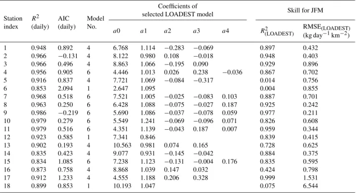
Table 2.Performance of LOADEST model in predicting the observed TN loadings from the WQN database. Models with linear time components (Model No.: 3, 5, 7–9) are not considered. The skill in predicting JFM WQN loadings is separately given in the last two columns.
Coefficients of
Skill for JFM
Station R2 AIC Model selected LOADEST model
index (daily) (daily) No.
a0 a1 a2 a3 a4 R(LOADEST)2 RMSE(LOADEST)
(kg day−1km−2)
1 0.948 0.892 4 6.768 1.114 −0.283 −0.069 0.897 0.432
2 0.966 −0.131 4 8.122 0.980 0.108 −0.018 0.948 0.403
3 0.966 0.496 4 8.863 1.066 −0.195 0.090 0.929 0.896
4 0.956 0.905 6 4.446 1.013 0.026 0.238 −0.036 0.867 0.702
5 0.916 0.837 4 7.721 1.069 −0.084 −0.317 0.014 0.756
6 0.853 2.094 1 2.647 1.095 0.004 0.855
7 0.968 0.518 6 7.521 1.005 −0.025 −0.083 0.103 0.887 0.701
8 0.963 0.250 6 6.428 1.088 −0.075 −0.027 0.187 0.925 0.242
9 0.986 −0.219 6 5.690 1.086 −0.037 −0.078 0.059 0.977 0.211
10 0.979 0.279 6 5.549 1.241 −0.069 −0.096 0.071 0.826 0.608
11 0.979 0.516 6 4.351 1.139 −0.043 0.187 0.007 0.959 0.344
12 0.923 0.585 1 7.341 0.846 0.839 0.415
13 0.902 0.193 4 10.563 0.981 0.074 0.165 0.728 0.625
14 0.835 0.423 4 9.077 0.931 −0.145 −0.042 0.884 0.375
15 0.834 1.085 6 7.238 1.123 −0.131 −0.004 0.176 0.835 0.595
16 0.873 0.758 4 8.868 1.039 0.147 0.032 0.424 0.798
17 0.912 1.233 4 4.555 1.188 0.206 0.328 0.999 1.531
18 0.899 0.853 1 10.193 1.047 0.075 6.544
dtime also represents the seasonality in loadings pattern. For a detailed expression ondtime, see Cohn et al. (1992).
The LOADEST model allows the user to select the best-fitting regression model from 11 predefined regression mod-els using the Akaike information criterion (AIC) (Akaike, 1974). Five regression models that include a linear time trend are not appropriate, since we are employing observed stream-flow to estimate simulated loadings beyond the observed pe-riod. Therefore, the simulated nutrient loadings based on the remaining regression models (i.e., model forms: 1, 2, 4 and 6 as defined in Runkel et al., 2004) in the LOADEST pro-gram do not have any time trend. Equation (1) represents the model form 6. Model form 1 (Eq. 1) considers only the first two (three) terms on the right-hand side (RHS) of Eq. (1), whereas model form 3 considers all the terms except the third term in the RHS of Eq. (1). For further details on model forms, see Runkel et al. (2004). Table 2 shows the goodness of fit statistics (coefficient of determination (R2)and AIC) in predicting the observed daily loadings in the WQN database (Table 1) and the coefficients of the best fitting regression model for TN for the selected 18 stations. From Table 2, we infer thatR2ranges from 0.83–0.97 indicating good fit of the observed daily loadings over 18 stations.
In this study, we primarily focus on developing nutrient forecasts for the winter season. Given that streamflow peaks in winter over the Southeast US, it has been shown that loadings are at their peak during the same season (Muller
and Spahr, 2006). From the perspective of winter forecasts too, this is a season that has significant skill in predict-ing observed precipitation by the ECHAM4.5 model (Devi-neni and Sankarasubramanian, 2010). Given that the selected 18 basins are virgin watersheds whose flows are minimally impacted by anthropogenic influences, the primary source of total nitrogen is from non-point that includes fall foliage and post-harvest agricultural lands (Muller and Spahr, 2006). Thus, increased flow during the winter season primarily car-ries the TN loadings from fall foliage and agricultural lands. Given the focus on the JFM season, we also report the ability of the LOADEST model in predicting the observed JFM nu-trients in Table 2. FromR(LOADEST)2 and RMSE during JFM, we clearly see that the performance of the LOADEST model in predicting JFM nutrients is poor in stations 5, 6, 13, 16 and 18. This potentially will have impact in developing nutrient forecasting model for the sites with lowR2in JFM.
LOADEST model, the simulated daily and the aggregated winter loadings are statistically unbiased (Cohn, 2005). We also computedR2(LOADEST) and the root-mean-square error (RMSE(LOADEST))for the simulated winter TN loadings
ob-tained from the LOADEST model. For additional details on computing errors in seasonal predictions, see Cohn (2005). Further, to ensure that there is no trend in the winter loadings, we performed Mann-Kendall test. At 1 % significance level, null-hypothesis with Kendall’s tau being not equal to zero was rejected in all of the sites for TN. We also performed regional Mann-Kendall test to account for spatial correlation among the 18 stations (Douglas et al., 2000). The p-value for TN is 4 % indicating no trend at the regional level. Our study will consider the simulated winter TN loadings (Lt) available during 1957–2009 for relating the interannual hy-droclimatic variability to nutrient variability over 18 stations in the SEUS.
2.4 Climate forecasts database
Seasonal climate forecasts are typically developed either using atmospheric GCMs (AGCMs) or using coupled GCMs (CGCMs). In the case of former, it is a two-tiered system, in which SSTs are forecasted first using a statistical/dynamical model and then they are forced with AGCMs. In CGCMs, since ocean and atmospheric models are coupled, they are run in a continuous mode. Recent studies clearly show that AGCMs are more skillful than CGCMs (Goddard et al., 2003). Further, Devineni and Sankarasubramanian (2010) show that ECHAM4.5 precipitation forecasts explain 25–36 % of the variability in observed precipitation over the Southeast US. For this study, we utilize the retro-spective winter precipitation forecasts from ECHAM4.5 general circulation model forced with constructed analogue SSTs (http://iridl.ldeo.columbia.edu/SOURCES/.IRI/.FD/ .ECHAM4p5/.Forecast/ca sst/.ensemble24/.MONTHLY/ .prec/, International Research Institute of Climate and Society (IRI) data library) (Li and Goddard, 2005). Ret-rospective precipitation forecasts from ECHAM4.5 are available for 5 months in advance for every month beginning January 1957. To force the ECHAM4.5 with SST forecasts, retrospective monthly SST forecasts were developed based on the observed SST conditions in that month based on the constructed analogue approach. For additional details on forcing ECHAM4.5 using constructed analogue SST forecasts, see Li and Goddard (2005).
Figure 1 also shows the locations of 56 grid points of pre-cipitation forecasts from ECHAM 4.5 along with their lati-tude and longilati-tude over SEUS. For this study, we utilize only the forecasted mean (which is obtained by computing the av-erage of 24 ensembles) of winter retrospective precipitation forecasts issued in the beginning of January for developing 3-month ahead retrospective nutrient forecasts over the period 1957–2007.
3 Low-dimensional models development and performance validation metrics
Given that winter streamflow over the SEUS is predomi-nantly rainfall driven with limited snow accumulation, we hypothesize that precipitation is the primary driver in con-trolling the JFM loadings. To verify this, we correlate simu-lated JFM loadings with both observed precipitation (Fig. 2a) and principal components of the forecasted precipitation from ECHAM4.5 (Table 3). Principal components basically signify the reduced dimensions of the gridded precipitation forecasts. Given that the precipitation forecasts from the se-lected grid points are spatially correlated, it is better to ob-tain low/reduced dimensions of the forecasts using principal component analysis. In this study, we only employ Spear-man rank correlation for performing all correlation analy-ses. Similarly, the computed rank correlation was checked for statistical significance (i.e., 1.96/(n−3)0.5at 95 % con-fidence interval, wherendenotes the number of data points used in calculating the correlation). Thus, the computed cor-relation in Fig. 2a needs to be greater than 0.29 (n=50) to
indicate statistically significant relationship between the ob-served precipitation and simulated loadings.
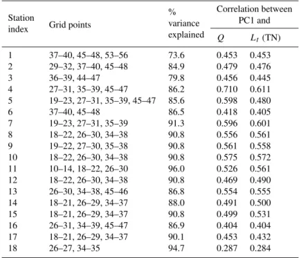
Table 3.Rank correlation between observed winter streamflow, TN loadings with the first principal component of the winter precipitation forecasts for the 18 selected stations. Locations of grid points indicated in the Table are shown in Fig. 1.
Station %
Correlation between
index Grid points variance
PC1 and
explained Q Lt(TN)
1 37–40, 45–48, 53–56 73.6 0.453 0.453
2 29–32, 37–40, 45–48 84.9 0.479 0.476
3 36–39, 44–47 79.8 0.456 0.445
4 27–31, 35–39, 45–47 86.2 0.710 0.611
5 19–23, 27–31, 35–39, 45–47 85.6 0.598 0.480
6 37–40, 45–48 86.5 0.418 0.405
7 19–23, 27–31, 35–39 91.3 0.596 0.601
8 18–22, 26–30, 34–38 90.8 0.556 0.561
9 19–22, 27–30, 35–38 90.8 0.561 0.558
10 18–22, 26–30, 34–38 90.8 0.575 0.572
11 10–14, 18–22, 26–30 96.0 0.526 0.561
12 18–22, 26–30, 34–38 90.8 0.469 0.490
13 26–30, 34–38, 45–46 86.8 0.554 0.555
14 18–21, 26–29, 34–37 88.0 0.491 0.500
15 18–21, 26–29, 34–37 90.8 0.499 0.531
16 26–31, 34–39, 45–47 86.9 0.404 0.404
17 18–21, 26–29, 34–37 90.1 0.453 0.432
18 26–27, 34–35 94.7 0.287 0.284
3.1 Source of climatic information influencing the winter TN variability
To understand the source of climate information that modu-lates the TN variability over the SEUS, we performed princi-pal component analysis on the simulated loadings (Lt)of TN over 18 stations. The first component approximately explains 59 % of total variability in TN loadings over 18 stations. It is well known in the hydroclimatic literature that ENSO is one of the important climatic conditions that influence the win-ter precipitation, temperature and streamflow over the SEUS (Ropelewski and Halpert, 1987). Figure 2b shows the cor-relation between the first component of JFM TN loadings over 18 stations and JFM Nino3.4 – an index used to de-note ENSO conditions by averaging the SSTs (Kaplan et al., 1998) over the tropical Pacific (170◦W–120◦W; 5◦S– 5◦N). From Fig. 2b, we infer that roughly 36 % of the vari-ability in the first principal component of nutrient loadings over SEUS could be explained purely based on ENSO con-ditions. ENSO plays an important role on the winter climate of the US since its peak activity typically coincides during December–February. In fact, the precipitation forecasts from ECHAM4.5 incorporate the forecasts of tropical SST ditions (i.e., Nino3.4 region), which are obtained from con-structed analogue SST forecasts for forcing the ECHAM4.5. Thus, ENSO is one of the sources of climatic variability that primarily influence both JFM hydroclimatic and nutri-ent variability over the SEUS. Based on the information pro-vided in Fig. 2 and Table 3, we understand that there is scope
for using the low-dimensional components of precipitation forecasts for developing season-ahead forecasts of TN load-ings over 18 selected stations.
3.2 Low-dimensional models
Given that our interest is primarily in understanding how large-scale hydroclimatic information could be utilized for seasonal nutrient predictions over the SEUS, we consider two low-dimensional models: principal component regres-sion (PCR) and canonical correlation analysis (CCA). Low-dimensional models reduce the correlated predictors and pre-dictands so that a subspace of uncorrelated predictors and predictands could be used for regression model development (Tippet et al., 2003; Sankarasubramanian et al., 2008). Fur-ther, these low-dimensional models also recalibrate the GCM forecasts so that any bias in predicting the JFM long-term mean of the nutrients is removed based on the regression model. Brief description of the low-dimensional models is provided next.
3.2.1 Principal component regression (PCR):
R² = 0.35
-6 -4 -2 0 2 4 6 8 10
-2.0 -1.5 -1.0 -0.5 0.0 0.5 1.0 1.5 2.0 2.5
P
C1 o
f
T
N
L
o
a
d
in
g
s
(
o
ve
r
18
S
tat
io
n
s
)
JFM Nino3.4 (a)
(b)
Fig. 2.Rank correlation between the simulated total nitrogen (TN)
loadings from the LOADEST model and observed precipitation(a)
and the association between El Ni˜no Southern Oscillation (ENSO) index – Nino3.4 – and the first principal component (PC1) of TN
loadings(b)over the selected 18 stations.
region are spatially correlated, employing precipitation fore-casts from multiple grid points as predictors would raise mul-ticollinearity issues in developing the regression. To avoid this, we employ PCR based on Eq. (2):
ln(Lt)= ˆβ0+
K X
k=1
ˆ
βj·PCkt + ˆεt (2)
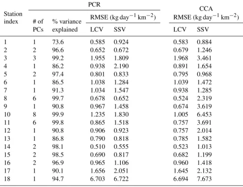
whereLt denotes the estimate of daily average TN loadings during the JFM season in yeart, PCkt denotes thek-th PCs from the retainedKPCs of precipitation forecasts andβˆs de-note the regression coefficients, whose estimates are obtained by minimizing the sum of squares of error. We employ step-wise regression to selectKPCs out of the rotated grid points of precipitation (given in Table 3) for developing the PCR model. From Table 4, we infer that most of the stations (ex-cept stations 8, 10 and 11) require only up to the first four principal components for developing the PCR model.
3.2.2 Canonical correlation analysis (CCA):
In PCR, we develop separate regression models for each site. Given that the predictands, the winter loadings, across the basins are also spatially correlated, one could utilize that information to develop a reduced set of regression models. CCA is a low-dimensional regression modeling framework that utilizes inter-site correlations to relate many (multiple predictands)-to-many (multiple predictors). Consider win-ter loadings available from m sites represented by LT=
(L1, L2,..., Lm) (dimension: nXm), whose corresponding
p grid points of precipitation forecasts (p > m) are repre-sented asXT=(X1, X2,...,Xp)(dimension:nXp)where “T” denotes the transpose. Then, canonical correlation analysis finds a linear combination of the p predictors, L∗=bTL,
that maximally correlates with the linear combination ofm predictands (X∗=aTX). Mathematically, the canonical cor-relation is obtained by choosing the vectorsaandbthat
max-imize the relationship
aTX
xy
b
!,(
aTX
xx
a
!
bTX
yy
b
!)1/2
where P
denotes the variance-covariance matrix between the two matrices in the subscript. For a detailed mathematical treatment of CCA, see Wilks (1995). Number of components frommpredictands andppredictors to be retained for the regression is decided based on step-wise regression. Squared values of canonical correlation represent the percentage of variance explained in each predictand by the predictors un-der that dimension. Thus, CCA allows us to develop a re-duced set of models that can be used to predict loadings for each site based on the precipitation forecasts.
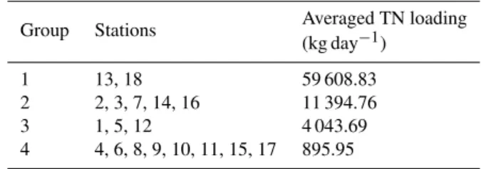
Before performing CCA, we first group the basins based on k-means clustering (Hartigan and Wong, 1979) so that CCA could be performed on each cluster. Based on cluster-ing, four groups were identified (Table 5) with the sites hav-ing the highest loadhav-ings placed under group 1 and the lowest average loadings placed under group 4. Separate CCA was performed for each group. For instance, CCA on group 1 is performed on loadings from two sites (m=2) and the
cor-responding grid points of precipitation forecasts for the two sites (# 13 and #18) from Table 3 are combined (p=20)
as predictors. The skill in predicting the winter loadings for each station is evaluated based on two different skill scores, which are discussed next.
3.3 Skill scores for nutrients forecasts
Table 4.Skill, expressed as root-mean-square error (RMSE) (based on Eq. 4), in predicting winter TN loadings using climate forecasts. Table also gives the number of principal components considered and the percentage variance explained by them for the total grid points selected (given in Table 3) for each station.
Station
PCR
CCA
index # of % variance RMSE (kg day
−1km−2) RMSE (kg day−1km−2)
PCs explained LCV SSV LCV SSV
1 1 73.6 0.585 0.924 0.583 0.884
2 2 96.6 0.652 0.672 0.679 1.246
3 3 99.2 1.955 1.809 1.968 3.461
4 1 86.2 0.938 2.190 0.891 1.654
5 2 97.4 0.801 0.833 0.795 0.968
6 1 86.5 1.038 1.284 1.039 1.472
7 1 91.3 1.034 1.547 0.938 1.285
8 6 99.7 0.678 0.652 0.524 2.319
9 1 90.8 0.967 1.458 0.674 3.619
10 8 99.9 1.235 1.830 1.005 6.453
11 6 99.8 0.865 1.518 0.757 3.691
12 1 90.8 0.906 0.923 0.757 2.014
13 1 86.8 0.790 0.818 0.785 1.582
14 2 98.1 0.510 0.555 0.523 1.013
15 2 98.5 0.690 0.817 0.682 1.199
16 2 96.9 0.965 1.106 0.960 1.418
17 1 90.1 1.656 2.051 1.645 2.132
18 1 94.7 6.703 6.722 6.694 7.673
(R2(LOADEST), RMSE(LOADEST)) (see Table 2) and the error in
predicting simulated JFM nutrients from LODEST based on the low-dimensional model(R(PCR/CCA)2 , RMSE(PCR/CCA)).
Since these two models are developed independently,R2and RMSE in predicting winter nutrient loadings using climate information could be expressed as follows:
R2=R(LOADEST)2 ·R(PCR/CCA)2 (3)
RMSE=(RMSE(LOADEST)+RMSE(PCR/CCA))/A (4)
For each station,R(PCR/CCA)2 and RMSE(PCR/CCA)were
com-puted based on the estimated TN loadings from the low-dimensional models and the simulated winter TN loadings for the period 1957–2006. Thus, we compute skill measures using Eqs. (3) and (4) to quantify our ability to explain the interannual variability in winter TN loadings using precipita-tion forecasts from ECHAM4.5.
4 Results and analyses
To ensure that the skill in forecasting winter nutrients is reli-able, we evaluate the low-dimensional models based on two different types of validation: leave-X out cross-validation (LCV) and split-sample validation (SSV). Both these meth-ods are commonly adapted in forecasting literature for vali-dating the model (Wilks, 1995).
4.1 TN loadings forecasts based on PCR models
Fig. 3. Box plot of R2 (based on Eq. 3) of principal compo-nent regression (PCR) model predicted TN loadings obtained using PCs of forecasted precipitation under leave-one-out cross validation (LCV).
the WQN database is greater than 0.29, which is statistically significant for the 51 yr of data considered. The forecasted TN loadings show statistically insignificant relationship with observed TN loadings that the correlation coefficients are 0.28 and 0.16 for stations 6 and 18 respectively. Poor good-ness of fit (see Table 2,R2(LOADEST)) from the LOADEST model is the primary reason behind the poor performance of these two stations during the winter season. Further, station 18 shows poor correlation between the principal components of precipitation forecasts and JFM loadings (Table 3). An-other possible reason for such poor prediction by LOADEST model in those two stations is the limited number of years of data availability (see Table 1) with station 6 (18) WQN obser-vations spanning 14 (12) years having a total of 56 (57) daily samples. The median RMSE (Table 4) computed under LCV also shows that error in predicting the observed WQN load-ings during the winter season is lesser than 1 kg day−1km−2 for most of the stations.
Under split-sample validation (SSV), PCR models are de-veloped usingLt and PCs available over the calibration pe-riod (PCR: 1957–1986) and skill measures are computed in predictingLt during the validation period (1987–2007). Hence,R2needs to be higher than 0.21 (correlation>0.46 for 21 yr of data) to demonstrate statistically significant skill in predicting season-ahead nutrient loadings. Based on this, Fig. 4 indicates that 11 stations (2–4, 7–11 and 13–15) show significant skill in predicting TN loadings. Stations 6 and 18 perform poorly because of the limited number of years of WQN data which results in very lowR2of the LOADEST model. Apart from these two stations, stations 1, 5, 12, 16 and 17 also show insignificant skill (R2<0.21). Stations 5 and 16 perform poorly due to the poor skill of the LOAD-EST model during JFM (see Table 2,R2(LOADEST)). Similarly, stations 1, 12 and 17 perform well under LCV, but the skill is statistically insignificant under SSV, even though the sim-ulated TN (Fig. 2) loadings exhibit significant correlation with both observed precipitation (Table 2) and forecasted
Table 5.Grouping of 18 selected stations based on k-means clus-tering.
Group Stations Averaged TN loading
(kg day−1)
1 13, 18 59 608.83
2 2, 3, 7, 14, 16 11 394.76
3 1, 5, 12 4 043.69
4 4, 6, 8, 9, 10, 11, 15, 17 895.95
precipitation (Table 3). It is important to discuss the impor-tance from the perspective of developing real-time nutrient forecasts. LCV basically exploits all the available data in the future years to predict the TN loadings for the left-out year. Thus, LCV shows that there is potential in developing sea-sonal nutrient forecasts for sites 1, 12 and 17. However, un-der SSV, we cannot guarantee that skill in developing real time (without using future information) forecasts, since the trained model using the data from 1957–1986, is not capable of developing a statistically significant forecast for the pe-riod 1987–2007. But, as we collect more data in the future, we may be able to develop statistically significant forecasts for these stations. Thus, LCV shows the potential skill in de-veloping the forecast, whereas SSV shows the demonstrable skill in developing real-time forecasts. Thus, based on two different validation methods, we understand that 11 stations (2–4, 7–11 and 13–15) exhibit statistically significant skill in predicting the observed WQN loadings using the PCR model developed separately for each site. Next, we evaluate the abil-ity to predict the loadings in these stations under a differ-ent low-dimensional model – canonical correlation analyses – that utilizes the spatial correlation in the TN loadings to develop a predictive model.
4.2 TN loadings forecasts based on canonical correlation analyses
Four different CCAs were performed on each group (listed in Table 5), and the developed models were evaluated un-der LCV and SSV. For LCV, we simply perform leave-5 out cross-validation instead of repeated fitting of the model (as described in Sect. 4.1 for the PCR model). Under leave-5 out cross-validation, we randomly leave out five predictands and predictors along with the year for which the prediction is desired for each station under a given group (in Table 5) and CCA model is developed using the rest of the 46 yr of data. The developed CCA model was employed to predict the year for which the prediction is desired. This procedure was repeated for all the years of observation under a given group to develop the CCA model estimated loadings. The RCCA2 and RMSECCAwere estimated between the simulated
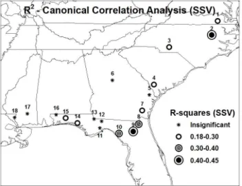
Fig. 4.ModifiedR2(based on Eq. 3) of PCR model predicted TN loadings obtained using PCs of forecasted precipitation under split sample validation (SSV).
according to Eqs. (3) (Fig. 5) and Eq. (4) (Table 4) to ac-count for the errors in the LOADEST model in predicting the WQN database. From Fig. 5, stations 5, 6 and 18 do not exhibit statistically significant correlation in predicting the loadings from the WQN loadings. As discussed under PCR model, stations 5, 6 and 18 did not perform well because of the limited number of years of WQN data and lowR2 of the LOADEST model during the winter season. The rest of the sites exhibited statistically significant relationships in ex-plaining the observed variability in the WQN loadings. For stations 8 and 9, CCA model explains 30–40 % (correlation 0.55–0.63) of the observed winter variability in TN within the WQN database. With regard to RMSE, the performance of CCA model and PCR model is almost similar at most of the stations having an error less than 1 kg day−1km−2.
Under SSV (Fig. 6 and Table 4), we computeR2 based on the predicted loadings during 1987–2007 using the CCA model developed over the period 1957–1986. From Fig. 6, CCA model did not exhibit any skill in predicting the win-ter loadings in stations 5, 6, 11–13, 16–18. Comparing this with the PCR model performance, the CCA model performs similarly with the exception being very lowR2at station 11. For station 11, PCR (R2=0.47) performs significantly bet-ter than the CCA model (R2=0.14). One possible reason for such poor performance of CCA model is that station 11 has low correlation with the rest of the sites under group #4 which has 8 stations. Under SSV,R2of the CCA model for the rest of the stations is almost similar to that ofR2of the PCR model. However, the RMSECCAis consistently higher
than the RMSEPCR (Table 4). This implies that the
condi-tional bias (overprediction and underprediction) of the CCA model is much higher. One possible reason for such increased conditional bias under CCA is due to increased heteroscedas-ticity in the observed loadings under a given group. However,
Fig. 5.ModifiedR2(based on Eq. 3) of canonical correlation anal-ysis (CCA) model predicted TN loadings obtained using PCs of forecasted precipitation under LCV.
the ability of the CCA model to explain the observed vari-ance in loadings is almost comparable to that of the PCR model, indicating that the source of interannual variability in winter nutrients is the same across the region. To sum-marize, using ECHAM4.5 precipitation forecasts alone, we infer both low-dimensional models demonstrate significant ability in predicting the observed winter TN loadings in nine coastal stations (#2–4, 7–10 and 14–15) based on two differ-ent validation methods.
5 Discussion
Analyses presented in Figs. 2–6 show that interannual vari-ability in nutrient loadings could be predicted well before the beginning of the season contingent on the climate forecasts.
Fig. 6.ModifiedR2(based on Eq. 3) of CCA model predicted TN loadings obtained using PCs of forecasted precipitation under SSV.
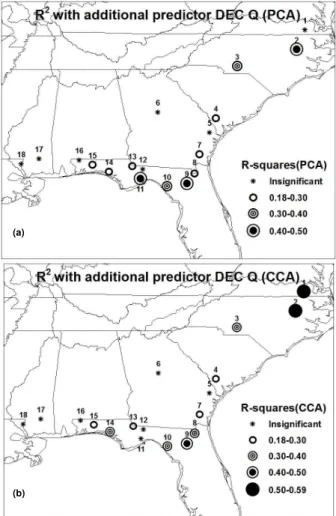
statistically significant skill by adding streamflow as an ditional predictor. However, by using streamflow as an ad-ditional predictor,R2 of the CCA model substantially im-proved over all stations, which indicates the importance of incorporating basin information in spatial-dimension reduc-tion. Further, RMSE of both PCR and CCA models is sub-stantially reduced by adding the observed December stream-flow as an additional predictor. This implies that antecedent storage/flow conditions are very critical in reducing the con-ditional bias in developing season-ahead TN forecasts result-ing in reduced over/underprediction compared to the mod-els developed using the precipitation forecasts alone. Thus, from a process control perspective, given the good skill in the reconstructed seasonal nutrient loadings, the interannual variability in nutrient loadings could be partially explained based on climatic variability. But, to obtain improved predic-tion (i.e., RMSE), it is important to incorporate both climatic variability and antecedent storage conditions in developing season-ahead nutrient forecasts.
5.1 Role of basin characteristics
We also compared the R2 (Fig. 7a) and RMSE (Table 6) to basin characteristics such as drainage area (figure not shown). But, we did not find any significant relationship be-tween the skills of the nutrient forecasts to basin character-istics. It is difficult to associate the spatial variability in the skill with the basin characteristics just using 18 stations. Fur-ther, at interannual time scales, we understand that climatic signals are the primary source of variability (Fig. 2b) fol-lowed by basin storage conditions (Fig. 7). Performing these analyses over the continental scale may provide additional information on the role of basin characteristics in influenc-ing the skill in predictinfluenc-ing nutrients.
Table 6.RMSE (Eq. 4) of forecasted TN loadings based on PCR and CCA models that consider ECHAM4.5 precipitation forecasts and December streamflow as predictors under SSV.
Station RMSE (kg area−1)
index PCR CCA
1 0.653 0.866
2 0.671 1.233
3 1.748 3.420
4 2.136 1.487
5 0.845 0.930
6 1.247 1.438
7 1.312 1.283
8 0.631 2.359
9 1.294 3.190
10 1.266 6.061
11 1.510 3.417
12 0.846 1.419
13 0.750 1.370
14 0.508 1.008
15 0.810 1.193
16 1.058 1.411
17 2.022 2.038
18 6.713 7.032
5.2 Validating nutrient forecasts with observed precipitation
(a)
(b)
Fig. 7.R2(based on Eq. 3) of PCR(a)and CCA(b)model pre-dicted TN loadings obtained using both PCs of forecasted precipi-tation and December streamflow under SSV.
is important to note that this false alarm rate also incorpo-rates the errors that would have resulted from the forecasted precipitation. Results from Table 7 show that the forecasted nutrients modulate well with the observed extreme seasons in precipitation over the validation period 1987–2007 and could be utilized for issuing categorical nutrient forecasts.
5.3 Potential for application – water quality trading
Perhaps the most important utility of the season-ahead fore-casts of nutrient loadings is in promoting water quality trad-ing. Some of the successful water quality trading programs in the country (e.g., Tar-Pamlico River Basin and Neuse River Basin in NC) typically allow trading nutrient loadings across different point sources as well as with non-point sources (e.g., farmers participating in the voluntary nutrient reduction program) through the basin-level trading association so that the seasonal/annual load caps are always met from the basin. Research on climate forecasts and water allocation clearly shows that probabilistic streamflow forecasts could be effec-tively utilized to specify the failure probability of reservoir
Table 7.The false alarm rate of nutrient forecasts developed using precipitation forecasts and December streamflow.
Station
Observation-index
Precipitation
BN AN
2 0.0 0.0
3 0.0 0.0
4 0.05 0.0
7 0.05 0.0
8 0.0 0.14
9 0.05 0.14
10 0.1 0.0
14 0.05 0.14
15 0.05 0.0
Average 0.04 0.05
releases as well as in ensuring the end of season target stor-age conditions being met with high probability (Sankarasub-ramanian et al., 2009). Similarly, in the context of seasonal water quality management, the developed forecasts of load-ings could be used to estimate the probability of violation of target loadings for the upcoming season (Towler et al., 2010; Borsuk et al., 2002). One could also develop an optimal nu-trient loading model such that the probability of violating the total loadings from multiple sources is within the acceptable level. Thus, utilizing season-ahead forecasts of nutrient load-ings and updating them throughout the season provide an op-portunity to develop adaptive nutrient control strategies that ensure target nutrient loadings and desired concentration.
5.4 Alternate forecasting models and nutrient forecasts for urbanized watersheds
Thus, the intent of this study is to understand how well cli-mate and basin storage conditions control the development of skillful forecasts of TN loadings and to evaluate the per-formance of two low-dimensional models in issuing season-ahead nutrient forecasts utilizing climate forecasts and basin storage conditions. In principle, the analyses provided here could also be extended with other sophisticated statistical models including nonparametric and Bayesian hierarchical models to estimate the entire conditional distribution of load-ings. Similarly, one could also develop nutrient forecasts by forcing the mechanistic water quality model with forecasted streamflow and water temperature, which in turn could be ob-tained based on dynamical downscaling (Leung et al., 1999) or statistical downscaling (Devineni et al., 2008) based on the climate forecasts.
reduction. However, to apply this approach for urban water-sheds with significant anthropogenic influences, the devel-oped model could be used to predict the upstream loadings for the undeveloped segment of the watershed. However, to estimate the loadings leaving the fully developed watersheds, one needs to know the loadings from the point sources so that net loadings leaving the watershed could be estimated in total. We are currently working on extending this approach with weather forecasts, so that point and non-point sources could be controlled in both virgin basins as well as in basins whose loadings are significantly impacted by anthropogenic influences.
6 Summary and conclusions
The study primarily focused on understanding the process controls in estimating winter nutrient loadings by consider-ing 18 HCDN watersheds over the SEUS. Given the discon-tinuous observed daily TN loadings, the study reconstructed simulated TN loadings using the LOADEST model for the winter season. The ability to predict these simulated load-ings was validated with two low-dimensional models that uti-lize winter precipitation forecasts and pre-season flow condi-tions.
Out of 18 stations, a total of 9 stations (#2–4, 7–10 and 14–15) exhibited statistically significant skill in predict-ing the observed winter nutrient loadpredict-ings under both low-dimensional models based on two different validation meth-ods. However, the reported skill in predicting the TN load-ings accounts for both error from the LOADEST model as well as the error from the low-dimensional models. Find-ings from the study could be summarized as the following “controls” that influence the skill in predicting seasonal TN loadings: stations that have very high R(LOADEST)2 (>0.8) in predicting the observed WQN loadings during the winter (Table 2) exhibit significant skill in loadings. This highR2 from the LOADEST model could be considered as a poten-tial criterion for developing nutrient forecasts if the basin’s hydroclimatology exhibits significant association with cli-matic signals. Incorporating antecedent flow conditions (De-cember flow) as an additional predictor did not increase the explained variance in these stations, but substantially reduced the RMSE in the predicted loadings. Understand-ing the source of climatic variability that controls the TN variability revealed that Nino3.4, an index denoting ENSO conditions over the tropical Pacific, accounted for 36 % of the observed spatial variability in the TN loadings over the SEUS. Given that using climate forecasts have been very beneficial in improving reservoir management over seasonal time scale (Sankarasubramanian et al., 2009), we argue the need to develop nutrient loading forecasts conditioned on cli-mate forecasts. Our future work will utilize these seasonal nutrient forecasts in developing adaptive water management plans over the SEUS.
Acknowledgements. The first author’s PhD dissertation research
was partially supported by the US National Science Foundation CAREER grant CBET-0954405. Any opinions, findings, and conclusions or recommendations expressed in this paper are those of the authors and do not reflect the views of the NSF. Authors also wish to thank Rob Runkel of USGS for his support in setting up the LOADEST model. Authors also wish to thank the two anonymous reviewers whose valuable comments led to significant improvements in the manuscript.
Edited by: C. de Michele
References
Alexander, R. B. and Smith, R. A.: Trends in the nutrient enrich-ment of US rivers during the late 20th century and their rela-tion to changes in probable stream trophic condirela-tions, Limnol. Oceanogr., 51, 639–654, 2006.
Alexander, R. B., Slack, J. R., Ludtke, A. S., Fitzgerald, K. K., and Schertz, T. L.: Data from selected US Geological Survey national stream water quality monitoring networks, Water Resour. Res., 34, 2401–2405, 1998.
Akaike, H.: A new look at the statistical model identification, IEEE T. Automat. Contr., 19, 716–723, 1974.
Arhonditsis, G. B., Winder, M., Brett, M. T., and Schindler, D. E.: Patterns and mechanisms of phytoplankton variability in Lake Washington (USA), Water Res., 38, 4013–4027, 2004.
Borsuk, M. E., Stow, C. A., and Reckhow, K. H.: Predicting the frequency of water quality standard violations: A probabilistic approach for TMDL development, Environ. Sci. Technol., 36, 2109–2115, 2002.
Borsuk, M. E., Stow, C. A., and Reckhow, K. H.: Confounding ef-fect of flow on estuarine response to nitrogen loading, J. Environ. Eng., 130, 605–614, 2004.
Chen, C. F., Ma, H. W., and Reckhow, K. H.: Assessment of wa-ter quality management with a systematic qualitative uncertainty analysis, Sci. Total Environ., 374, 13–25, 2007.
Childers, D. L., Boyer, J. N., Davis, S. E., Madden, C. J., Rudnick, D. T., and Sklar, F. H.: Relating precipitation and water man-agement to nutrient concentrations in the oligotrophic “upside-down” estuaries of the Florida Everglades, Limnol. Oceanogr., 51, 602–616, 2006.
Cho, H. J. and Poirrier, M. A.: Response of submersed aquatic vegetation (SAV) in Lake Pontchartrain, Louisiana to the 1997– 2001 El Ni˜no Southern Oscillation shifts, Estuaries, 28, 215–225, 2005.
Cohn, T. A.: Estimating contaminant loads in rivers: An application of adjusted maximum likelihood to type 1 censored data, Water Resour. Res., 41, W07003, doi:10.1029/2004WR003833, 2005. Cohn, T. A., Caulder, D. L., Gilroy, E. J., Zynjuk, L. D., and
Sum-mers, R. M.: The Validity of a Simple Statistical-Model for Esti-mating Fluvial Constituent Loads – an Empirical-Study Involv-ing Nutrient Loads EnterInvolv-ing Chesapeake Bay, Water Resour. Res., 28, 2353–2363, 1992.
Dettinger, M. D. and Diaz, H. F.: Global characteristics of stream flow seasonality and variability, J. Hydrometeorol., 1, 289–310, 2000.
combi-nations of coupled GCMs, Geophys. Res. Lett., 37, L24704, doi:10.1029/2010GL044989, 2010.
Devineni, N., Sankarasubramanian, A., and Ghosh, S.: Multi-model ensembles of streamflow forecasts: Role of predictor state in developing optimal combinations, Water Resour. Res., 44, W09404, doi:10.1029/2006WR005855, 2008.
Douglas, E. M., Vogel, R. M., and Kroll, C. N.: Trends in Flood and Low Flows in the United States, J. Hydrol., 240, 90–105, 2000. Hartigan, J. A. and Wong, M. A.: Algorithm AS 136: A k-means
clustering algorithm, Appl. Statist., 28.1, 100–108, 1979. Kaplan, A., Cane, M., Kushnir, Y., Clement, A., Blumenthal, M.,
and Rajagopalan, B.: Analyses of global sea surface temperature 1856–1991, J. Geophys. Res., 103, 18567–18589, 1998. Goddard, L., Barnston, A. G., and Mason, S. J.: Evaluation of the
IRI’s “net assessment” seasonal climate forecasts 1997–2001, B. Am. Meteorol. Soc., 84, 1761–1781, 2003.
Leung, L. R., Hamlet, A. F., Lettenmaier, D. P., and Kumar, A.: Simulations of the ENSO Hydroclimate Signals in the Pacific Northwest Columbia River Basin, B. Am. Meteorol. Soc., 80, 2313–2329, 1999.
Li, S. and Goddard, L.: Retrospective Forecasts with the ECHAM4.5 AGCM, IRI Technical Report, 05-02, 2005. Lin, J., Xie, L., Pietrafesa, L. J., Ramus, J. S., and Paerl, H. W.:
Wa-ter quality gradients across Albemarle-Pamlico estuarine system: Seasonal variations and model applications, J. Coastal Res., 23, 213–229, 2007.
Meybeck, M.: Carbon, Nitrogen, and Phosphorus Transport by World Rivers, Am. J. Sci., 282, 401–450, 1982.
Mueller, D. K. and Spahr, N. E.: Nutrients in Streams and Rivers across the nation-1992–2001, USGS Scientific Investigations Report, 2006.
Mueller, D. K., Ruddy, B. C., and Battaglin, W. A.: Logistic model of nitrate in streams of the upper-midwestern United States, J. Environ. Qual., 26, 1223–1230, 1997.
National Research Council: Assessing the TMDL approach to water quality management, 2001.
National Research Council: Florida Bay Research Programs and Their Relation to the Comprehensive Everglades Restoration Plan, 2002.
Paerl, H. W., Valdes, L. M., Peierls, B. L., Adolf, J. E., and Harding, L. W.: Anthropogenic and climatic influences on the eutrophica-tion of large estuarine ecosystems, Limnol. Oceanogr., 51, 448– 462, 2006.
Ropelewski, C. F. and Halpert, M. S.: Global and Regional Scale Precipitation Patterns Associated with the El-Ni˜no Southern Os-cillation, Mon. Weather Rev., 115, 1606–1626, 1987.
Runkel, R. L., Crawford, C. G., and Cohn, T. A.: Load Estimator (LOADEST): A FORTRAN Program for Estimating Constituent Loads in Streams and Rivers, US Geological Survey Report, 2004.
Sankarasubramanian, A., Sharma, A., Lall, U., and Espinueva S.: Role of retrospective forecasts of GCMs forced with persisted SST anomalies in operational streamflow forecasts development, J. Hydrometeor., 9, 212–227, 2008.
Sankarasubramanian, A., Lall, U., Souza Filho, F. D., and Sharma, A.: Improved Water Allocation utilizing Probabilis-tic Climate Forecasts: Short Term Water Contracts in a Risk Management Framework, Water Resour. Res., 45, W11409, doi:10.1029/2009WR007821, 2009.
Slack, J. R., Lumb, A., and Landwehr, J. M.: Hydro-Climatic Data Network (HCDN) Streamflow Data Set, 1874–1988, US Geolog-ical Survey Report, 1993.
Smith, R. A., Schwarz, G. E., and Alexander, R. B.: Regional inter-pretation of water-quality monitoring data, Water Resour. Res., 33, 2781–2798, 1998.
Smith, R. A., Alexander, R. B., and Schwarz, G. E.: Natural back-ground concentrations of nutrients in streams and rivers of the conterminous United States, Environ. Sci. Technol., 37, 3039– 3047, 2003.
Tippett, M. K., Anderson, J. L., Bishop, C. H., Hamill, T. M., and Whitaker, J. S.: Ensemble square-root filters, Mon. Weather Rev., 131, 1485–90, 2003.
Towler, E., Rajagopalan, B., and Summers, R. S.: Using Paramet-ric and NonparametParamet-ric Methods to Model Total Organic Carbon, Alkalinity, and pH after Conventional Surface Water Treatment, Environ. Eng. Sci., 26, 1299–1307, 2009.
Towler, E., Rajagopalan, B., Summers, R. S., and Yates, D.: An approach for probabilistic forecasting of seasonal turbid-ity threshold exceedance, Water Resour. Res., 46, W06511, doi:10.1029/2009WR007834, 2010.
Vecchia, A. V.: Relation Between Climate Variability and Stream Water Quality in the Continental United States, Hydrological Science and Technology, 19, 77–98, 2003.
Vitousek, P. M., Aber, J.D., Howarth, R. W., Likens, G. E., Mat-son, P. A., Schindler, D. W., Schlesinger, W. H., and Tilman, G. D.: Human alteration of the global nitrogen cycle: Sources and consequences, Ecol. Appl., 7, 737–750, 1997.