www.ocean-sci.net/5/475/2009/
© Author(s) 2009. This work is distributed under the Creative Commons Attribution 3.0 License.
Ocean Science
Enhancing temporal correlations in EOF expansions for the
reconstruction of missing data using DINEOF
A. Alvera-Azc´arate1,2, A. Barth1,2, D. Sirjacobs3, and J.-M. Beckers1
1AGO-GHER, University of Li`ege, All´ee du Six Aoˆut, 17, Sart Tilman, Li`ege, 4000, Belgium 2National Fund for Scientific Research, FNRS-FRS, Belgium
3Department of Life Sciences, University of Li`ege, Sart Tilman, Li`ege, 4000, Belgium Received: 15 June 2009 – Published in Ocean Sci. Discuss.: 9 July 2009
Revised: 9 October 2009 – Accepted: 14 October 2009 – Published: 28 October 2009
Abstract. DINEOF (Data Interpolating Empirical Orthogo-nal Functions) is an EOF-based technique for the reconstruc-tion of missing data in geophysical fields, such as those pro-duced by clouds in sea surface temperature satellite images. A technique to reduce spurious time variability in DINEOF reconstructions is presented. The reconstruction of these im-ages within a long time series using DINEOF can lead to large discontinuities in the reconstruction. Filtering the tem-poral covariance matrix allows to reduce this spurious vari-ability and therefore more realistic reconstructions are ob-tained. The approach is tested in a three years sea surface temperature data set over the Black Sea. The effect of the filter in the temporal EOFs is presented, as well as some ex-amples of the improvement achieved with the filtering in the SST reconstruction, both compared to the DINEOF approach without filtering.
1 Introduction
DINEOF (Data INterpolating Empirical Orthogonal Func-tions) is a technique to reconstruct missing data in geo-physical data sets using an EOF basis to infer the missing data (Beckers and Rixen, 2003). This technique is typi-cally applied to satellite data with gaps due to, for exam-ple, clouds present in the atmosphere that impede the sur-face IR radiation to reach the satellite sensor. Even in satel-lite measures taken with microwave-based sensors (such as the SST provided by TRMM (Tropical Rainfall Measuring
Correspondence to:A. Alvera-Azc´arate ([email protected])
Mission) Microwave Imager (TMI) satellites, or the Ad-vanced Microwave Scanning Radiometer (AMSR-E), http: //www.remss.com, Gentemann et al., 2004) large gaps can be present in rain zones and at days when the satellite swath does not completely cover the zone of study.
These clouds and gaps can obscure almost completely the studied domain, with a few clustered observations remaining in some parts of it. These observations are therefore not rep-resentative of the whole spatial variability of the domain, and an EOF decomposition, such as the one realised within DI-NEOF to retrieve missing data, can result in an over-fitting of the EOFs to the few present data. As a consequence the reconstructed image does not necessarily reflect the spatial variation of that given image. Satellite data sets typically used for reconstruction with DINEOF may contain some im-ages with the characteristics mentioned above. It is therefore possible that the reconstruction presents some discontinuities in time (i.e. consecutive images with very different values), because of the presence of these highly clouded images. We propose a filter that, applied to the temporal covariance ma-trix of the data before the EOF decomposition step in DI-NEOF, will reduce the temporal discontinuities in the tem-poral EOFs and therefore in the reconstructed data set.
2003
0
2004
2005
2006
20
40
60
80
100
%
30oE 34oE 38oE 42oN
44oN 46oN
BA
CR
%
Sea of Azov
60
65
70
75
80
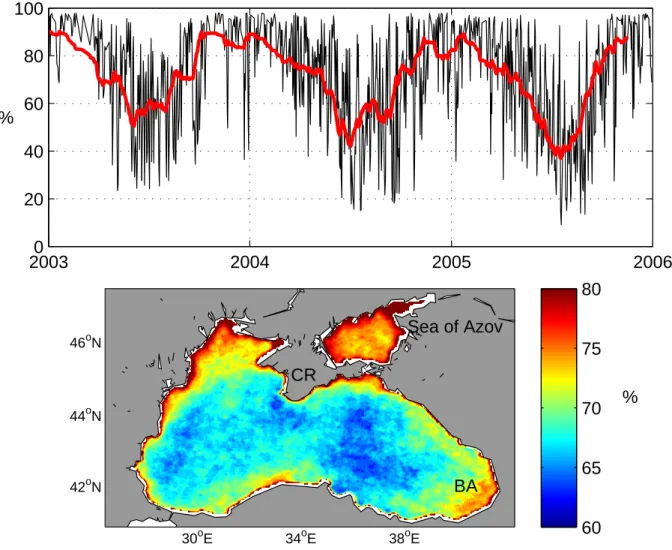
Fig. 1.Top panel: temporal variation of cloud cover percentage in the Black Sea (in black) and with a low-pass filter of 30 days (red line). The year labels show the 1st January of each year. Bottom panel: spatial variation of cloud cover percentage in the Black Sea. CR stands for Crimean peninsula, and BA stands for Batumi region.
2 Data
Daily night-time Sea Surface Temperature (SST) data of the Black Sea spanning from 1 January 2003 to 31 December 2005 are used in this work. The data are obtained through Advanced Very High Resolution Radiometer (AVHRR) sen-sors on board the NOAA Polar Orbiting Environmental Satellite series. They are available at the Jet Propulsion Lab-oratory (JPL) PODAAC website (http://podaac.jpl.nasa.gov). The horizontal resolution is 4.8 km. Images with cloud cover larger than 98% are not used for the analysis, and therefore the final temporal size is 903 (out of the initial 1096 images). The average cloudiness of this data set is about 70%. Tem-poral variability of total cloud cover presents an annual cycle with minimum average cloud cover of about 40 to 50% in summer and maximum average cloud cover of about 90% in winter (Fig. 1). Note the very high cloudiness in winter of
in-dividual time frames in this figure. Spatially, regions with the highest cloud cover percentage are the Sea of Azov and the northwestern shelf of the Black Sea, with an average cloud cover higher than 75%. In the rest of the Black Sea, the aver-age cloud cover varies from 60 to 80%. Typical cloud sizes are very large, covering most of the Black Sea at a time.
3 Methods
3.1 DINEOF
anomaly). Starting with the calculation of the most dominant EOF mode of this matrix, the missing data are calculated by:
Xm,n=Um,161VTn,1 (1)
withm=1...Mandn=1...N. Uare the spatial modes,V are the temporal modes and6 are the singular values. This new estimation for the missing data is reintroduced in the data matrix, and the EOF mode calculation is repeated. This process is repeated until convergence of the missing values, and then the EOF modes calculated are increased to two, then three, etc. The EOF mode calculation is done using a Lanczos solver provided by Toumazou and Cretaux (2001), which uses the ARPACK freeware (Lehoucq et al., 1997). The optimal number of EOF modes retained are calculated by cross-validation (i.e., a few valid data are set aside and the error of the reconstruction is assessed by comparing the reconstructed data to these cross-validation data).
To test the new filtering approach, the data used for cross-validation are not taken randomly as it is done in DINEOF by default (e.g. Beckers and Rixen, 2003; Alvera-Azc´arate et al., 2005, 2007). For this work, the 15 cleanest images are artificially covered by clouds extracted from other images, following the approach described in Beckers et al. (2006). Three percent of data is covered in this way for the cross-validation. The cross-validation clouds are a more realistic case than the random points, and therefore the reconstruction of the cross-validation data is done in the same conditions as the rest of the missing data. The cross-validation error using this approach can be expected to be a more realistic estimation of the reconstruction error.
Concerning the anomalies calculated within DINEOF, a space and time average is subtracted from the data to com-pute them. This choice guarantees that the method is sym-metric in space and time. In addition, it allows to com-pute anomalies in any data set, without prior knowledge of its variability. For satellite SST, it can be useful to remove e.g. the annual cycle, and provide these anomalies to DI-NEOF to reconstruct the missing data. However, when the annual cycle is not removed from the initial data, the EOF decomposition identifies this as the most dominant signal, so the first EOF contains in most cases the annual cycle. One can see the EOF decomposition then as a way to separate the annual cycle from the rest of the variability of the data set. In this work we chose not to remove the annual cycle from the data, but rather the general spatial and temporal mean. This way, the effect of the new proposed filter can be assessed in-dependently, as removing a different average might have also an impact on the reconstructed data.
For an extended description of DINEOF, and recent devel-opments, the reader is referred to Beckers and Rixen (2003); Azc´arate et al. (2005); Beckers et al. (2006); Alvera-Azc´arate et al. (2007).
3.2 Filtering the covariance matrix
MatrixX(if complete) can be filtered in the time domain as follows:
˜
X=XF (2)
whereFis aN×Nmatrix containing the filter. A singular value decomposition (SVD) of the filtered matrixX˜ can be calculated:
FTXTXFV˜ = ˜XTX˜V˜ = ˜V6˜ (3) The temporal covariance matrix is defined as:
B=XTX (4)
Therefore, Eq. (3) can be also written as:
FTBFV˜ = ˜BV˜ = ˜V6˜ (5)
where we made appear the filtered covariance matrix ˜
B=FTBF.
The filter F is implemented as a Laplacian filter on the terms of X, in which the temporal increment between two images is also taken into account: two consecutive images in matrixXwith a large time gap between them are less related than two consecutive images that are in addition consecutive in time. The latest will be more strongly weighted to each other than the first mentioned case. Considering a vectorx
containing the data to be filtered, the filter can be expressed as follows:
xi(s+1)=xi(s)+Gi+1−Gi
ti′+1−ti′ (6)
wherei=1...N,s=1...p, and
Gi =α
xi−xi−1
ti−ti−1
(7)
ti′= ti−1+ti
2 (8)
αis a parameter specifying the strength of the filter,t is a vector containing the time andxis a vector containing the data, all of lengthN. The filter is applied first to the columns ofBand then to its rows, according to Eq. (5). This step can be easily incorporated to DINEOF, before the SVD decom-position. FilteringBinstead ofXis more appropriate since Bis much smaller and is less sensitive to missing data.
The filter in Eq. (6) implies three consecutive terms of the times series. The reach of the filter can be increased by it-eratively reapplying it a predefined number of times. This iteration acts then over 2p+1 members, withpthe number of iterations of the filter.
0 5 10 15 20 25 30 35 40 45 50 0.4
0.5 0.6 0.7 0.8 0.9 1
# of EOFs
°C
Reference 1 iteration 3 iterations 10 iterations 30 iterations 100 iterations
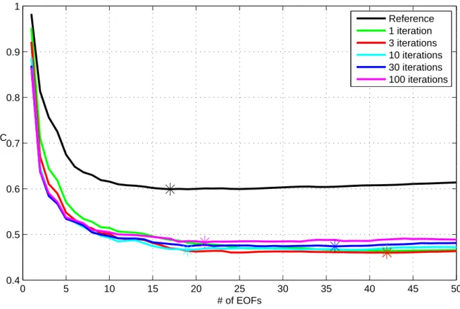
Fig. 2. Cross-validation error decreasing with the increasing number of EOFs used for the reconstruction. The minimum error is marked with an asterisk for each line. The lines show the cross-validation error for DINEOF without filtering, and for DINEOF with filtering of the covariance matrix using 1, 3, 10, 30 and 100 iterations of the filter.
(ifα>min(1t )2 2 the filter will be unstable) and the value for
pwas then decided by considering the cross-validation error provided by DINEOF. Figure 2 shows the cross-validation error for the reference run using DINEOF, and for five runs (withp=1,3,10,30 and 100) with the filter included in DI-NEOF. The use of the filter, for all values of p, produces a smaller cross-validation error than the reference run. Of all the five runs with the filter, it appears that p=3 gives the best reconstruction, which means that frequencies higher than 2π√αp=1.1 days are being filtered from the data set. Note that the choice of the number of iterations can be con-sidered as a fine-tuning experiment to obtain the smallest cross-validation error, as all experiments with filtering ob-tained better cross-validation error than the non-filtered ver-sion.
4 Results
4.1 Analysis of the covariance matrix
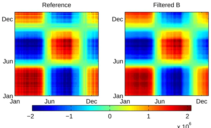
Figure 3 shows the covariance matrixB=XTX(non filtered – left panel – and filtered – right panel –) for the 2003 Black Sea SST data reconstructed using DINEOF. The diagonal in
this matrix represents the variance of each day’s data with re-spect to the mean of the data set. We can see a high variance in summer and winter, with spring and fall nearer to the av-erage temperature, and therefore with a lower variance. The off-diagonal terms are related to the degree of similitude of each image with respect to the rest of the images (or covari-ance), so winter is negatively correlated with summer, for example. The comparison between the left and right panels allows to see the effect of the filtering in the covariance ma-trix. In the non-filtered covariance matrix, discontinuities in the form of vertical and horizontal lines of low correlation are apparent. These discontinuities are caused by the irregu-larities in time and space mentioned above, and can lead to an unrealistic reconstruction of the data. The filtered version ofB, which is used within DINEOF in the version presented in this work, eliminates or reduces some of these discontinu-ities (Fig. 3 right).
4.2 EOF mode analysis
Reference
Jan
Jun
Dec
Jan
Jun
Dec
Filtered B
Jan
Jun
Dec
Jan
Jun
Dec
−2
−1
0
1
2
x 10
6Fig. 3.Temporal covariance matrix of the 2003 Black Sea SST reconstructed using DINEOF. Left panel: without filtering; right panel: with the application of the embedded filter. The labels indicate the first day of each month.
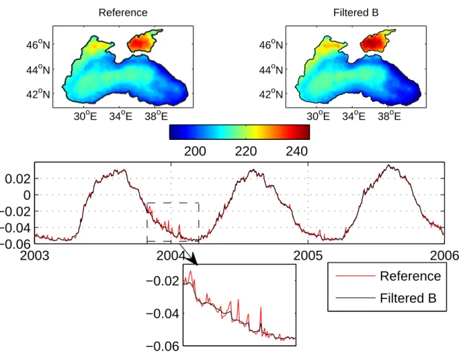
matrix. The filter is applied in the time dimension, therefore the spatial structure of the first EOF mode is very similar in both approaches. The first temporal mode of Fig. 4, how-ever, does present a difference between both reconstructions. While representing the annual cycle of cooling and warming temperatures in both reconstructed data sets, the non-filtered version presents several peaks at moments when the cloud coverage of the original data set is higher, for example dur-ing winter months. These peaks are smoothed in the filtered DINEOF version, which will lead to smoother reconstruc-tions in time, as it will be shown later. The first EOF mode (accounting for 98.11% of the total variability) represents the annual cycle variations of the Black Sea SST, because as we mentioned in Sect. 3.1, this cycle was not removed from the initial data. The cyclonic, coastal-trapped, basin-wide Rim Current is the most prominent feature in the spatial maps of Fig. 4. This current presents the warmest temperature during winter, and it is colder than it surroundings during summer, in part influenced by coastal upwelling along the Turkish coast (Sur and Ilyin, 1997) and the Crimean peninsula (Sur and Ilyin, 1997; Gawarkiewicz et al., 1999). The coldest regions during winter are the northwestern shelf and the Sea of Azov, exposed to rapid temperature changes related to the atmo-spheric conditions due to its shallow bathymetry (Sur et al., 1996; Kosarev et al., 2008).
The second EOF is shown in Fig. 5. The smoothing of the temporal EOF is more evident here than in the first EOF, and again the spatial modes present the same structure. The sec-ond temporal mode presents a semi-annual periodicity and a northeast-southwest spatial structure, mainly separating the Sea of Azov and the northwestern shelf from the south-east Black Sea. This mode accounts for a warming/cooling anomaly in spring/fall in the northwest shelf, and the oppo-site trend for the southeast zone of the Black Sea. This mode accounts for almost 1% of the total variability (or 53% of the remaining variability of modes of higher order than the first mode).
The third EOF mode, accounting for only 0.3% of the total variability (or 34% of the remaining variability of modes of higher order than the first and second modes), is presented in Fig. 6. The same comments as for the other modes stand here, as the spatial mode is almost the same for the filtered and non-filtered versions of DINEOF, and the temporal mode is smoother in the filtered DINEOF version.
4.3 SST Reconstruction
30oE 34oE 38oE 42oN
44oN 46oN
Reference
30oE 34oE 38oE 42oN
44oN 46oN
Filtered B
200
220
240
2003
2004
2005
2006
−0.06
−0.04
−0.02
0
0.02
Reference
Filtered B
−0.06
−0.04
−0.02
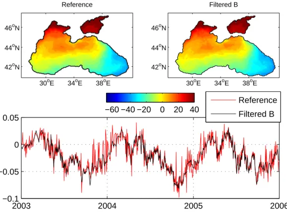
Fig. 4. First EOF spatial mode for the DINEOF reconstruction with no filtering of the covariance matrix (top left), with filtering of the covariance matrix (top right) and first temporal mode for both versions (bottom). The x-axis labels in the bottom panel indicate the 1st January of each year. The spatial EOF has units of◦C and the temporal EOFs have no units.
explained variance of 99.92%. When the filter of the covari-ance matrix is included, 42 EOF modes are retained, with a minimal cross-validation error of 0.46◦C, and a total ex-plained variance of 99.93%. It might appear surprising that when the filtering is included, more EOF modes are retained by DINEOF, although this can be explained by these modes being better constrained (i.e. determined) because the filter introduces information about the temporal sequence of the data. Also, note that the cross-validation error obtained with the inclusion of the filter is close to the accuracy of satellite SST data, when compared to in situ data (e.g. McClain et al., 1985; Kumar et al., 2000; Marullo et al., 2007; Castro et al., 2008).
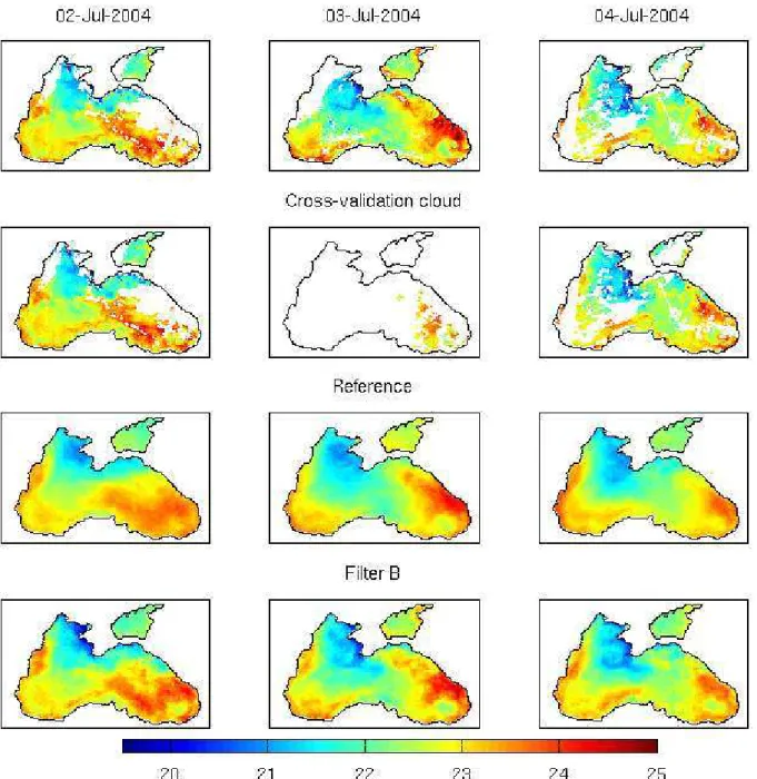
In Fig. 7 a sequence of initial data and reconstructions is shown. An example when a cross-validation cloud has been added is shown, so that readers can see the original data (first row of Fig. 7) and the data set used for the reconstruction (second row). Of course the three days shown are only a small part of the whole 903 images used in this work. The third row in Fig. 7 shows the reconstructed data using
30oE 34oE 38oE 42oN
44oN 46oN
Reference
30oE 34oE 38oE 42oN
44oN 46oN
Filtered B
−60 −40 −20
0
20 40
2003
2004
2005
2006
−0.1
−0.05
0
0.05
Reference
Filtered B
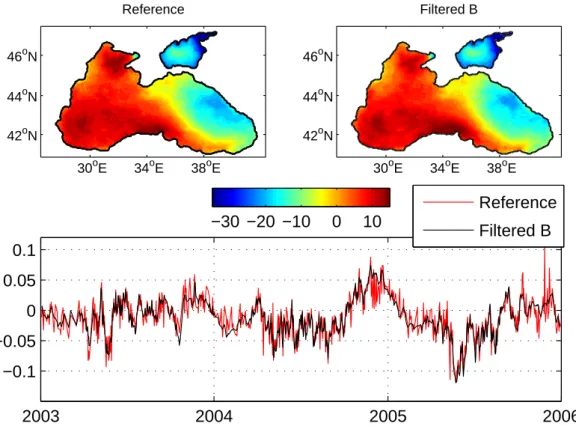
Fig. 5. Second EOF spatial mode for the DINEOF reconstruction with no filtering of the covariance matrix (top left), with filtering of the covariance matrix (top right) and second temporal mode for both versions (bottom). The x-axis labels in the bottom panel indicate the 1st January of each year. The spatial EOF has units of◦C and the temporal EOFs have no units.
the example given in Fig. 7 there are features that are also better represented in the filtered version of DINEOF, as the warm filament going from the Bosphorus strait to the Cape Kerempe, and the cold eddy in the Batumi region (southeast Black Sea).
Another example of the effect of the covariance matrix filtering on the reconstruction results can be seen in Fig. 8. The initially cloudy data from 24, 25 and 27 December 2003 present a large cloud cover on the last two days. On 25 De-cember, only a few data near the east coast of the Black Sea are cloudless, which represent values typically warmer than the western part in this period of the year. The reconstruction using DINEOF with no filtering leads to a very warm recon-struction on 25 December. The temperature change of up to 6◦C within one day observed in the classic reconstruction is not realistic in the Black Sea. The reconstruction using the filtering of the covariance matrix leads to a more real-istic result, with a temperature distribution similar to what is observed on 24 December 2003. On 27 December (the next day in the reconstructed images sequence), the informa-tion available in the initial matrix is from the colder western Black Sea. The reconstruction without the filtering leads to
cold SST over the whole Black Sea, and the southeastern part of the basin does not present warmer water as it would be ex-pected from past information. The filtered DINEOF recon-struction does present this east-west gradient, with warmer temperatures in the southeast and colder in the west.
30oE 34oE 38oE 42oN
44oN 46oN
Reference
30oE 34oE 38oE 42oN
44oN 46oN
Filtered B
−30 −20 −10
0
10
2003
2004
2005
2006
−0.1
−0.05
0
0.05
0.1
Reference
Filtered B
Fig. 6. Third EOF spatial mode for the DINEOF reconstruction with no filtering of the covariance matrix (top left), with filtering of the covariance matrix (top right) and third temporal mode for both versions (bottom). The x-axis labels in the bottom panel indicate the 1st January of each year. The spatial EOF has units of◦C and the temporal EOFs have no units.
gyre presents lower temperatures than observed, and in gen-eral, the spatial structures are much smoother than when the filter is applied within DINEOF. Note that the same proce-dure (i.e. a cross-validation error calculation) has been used to establish the number of iterations that yield the best results in the embedded filter and the a posteriori filter. When the fil-ter is applied a posfil-teriori a much higher number of ifil-terations is needed to obtain an accurate result. This is because the a posteriori filter has to counterbalance the effect of the noisy temporal EOFs that lead to the reconstruction in the second row of Fig. 8, whereas the embedded filter prevent the tem-poral EOFs to become noisy in the first place.
4.4 Effect of the number of EOFs on the reconstructions
The increased accuracy obtained with DINEOF when includ-ing the filter of the covariance matrix can be due to two rea-sons: the filtering of spikes on the temporal EOFs, and the increased number of EOFs that were retained in the Black Sea example shown here. To elucidate which of these ef-fects account for the improvements seen in Figs. 7 and 8, we have repeated the DINEOF reconstruction without filter, but forcing DINEOF to retain the same number of EOF modes
than with the filter (i.e. 42 EOF modes). As it might be expected, this reconstruction is able to better represent the small-scale variability of Fig. 7, to an extent that the recon-struction with and without filter present very similar results (the new results are not shown). However, this new recon-struction does still present the very warm reconrecon-struction on 25 December 2003, and in general, it exhibits spurious high frequency variations (as those seen in the temporal EOFs of Figs. 4 to 6). The cross-validation error of the classic DI-NEOF reconstruction retaining 42 EOF modes is of 0.61◦C (i.e., higher than the reconstruction with 17 EOFs, and higher than the reconstruction with the filter). These results confirm that the filtering of the covariance matrix is able to reduce the spikes in the temporal EOFs, therefore obtaining more realis-tic reconstructions. The increased number of EOFs retained when including a filter within DINEOF accounts for a better reconstruction of the small-scale features.
Fig. 7.Example of large cloud added for the cross-validation. Top row: initial cloudy data at three consecutive days, 2 to 4 July 2004. Second row: the same data set, but with a cross-validation cloud added on the 3rd July 2004, used for the reconstruction. Third row: reconstruction using no filtering of the covariance matrix. Fourth row: reconstruction with filtering of the covariance matrix.
for those reconstructions. The higher order EOFs do not only contain small-scale information, but also noise, so forc-ing DINEOF to retain a higher number of EOFs than what is calculated with the cross-validation method is not to be done without caution, as it might degrade the overall accu-racy of the reconstruction. The cross-validation approach used within DINEOF might however not be optimal, retain-ing less EOFs than necessary. This remains an open question that will be addressed in future work.
5 Conclusions
Fig. 8.SST initial data on 24, 25 and 27 December 2003 (top row) and two reconstruction by DINEOF: with no filtering of the covariance matrix (second row) and with filtering of the covariance matrix (third row). The last row show the result of a temporal filter applied after the reconstruction (i.e. to the data shown in the second row).
temporal covariance matrix of the data, before the temporal EOFs are calculated and used to infer the missing data values. It has been shown that the reconstruction of missing data is improved when this filter is embedded within DINEOF. The temporal information is taken into account in the reconstruc-tion, avoiding large discontinuities between two consecutive reconstructed images. The results obtained have been com-pared to a DINEOF reconstruction without the filter. The error of the reconstruction, as measured by cross-validation, is lower when the filter is embedded in DINEOF (0.6◦C ver-sus 0.46◦C when the filter is used). In addition, the temporal EOFs are better constrained, and as a result more EOFs are retained by DINEOF. This in turn increases the spatial vari-ability of the reconstructed data.
The combination of a lower reconstruction error and a higher number of temporal EOFs retained for estimating the missing values results in an improved estimation of the oceanographic features on the Black Sea sea surface temper-ature. An example has been shown in which a filament south of the Crimean peninsula was more accurately represented in the filtered reconstruction, because of the presence of this filament in the surrounding images, an information not ex-ploited in the reconstruction with no filter.
Acknowledgements. This work was realised in the context of the RECOLOUR (REconstruction of COLOUR scenes) – SR/00/111, and BELCOLOUR-2 (SR/00/104) projects funded by the Belgian Science Policy (BELSPO) in the frame of the Research Program For Earth Observation “STEREO II”. AVHRR SST data were obtained from the Physical Oceanography Distributed Active Archive Center (PODAAC) at the NASA Jet Propulsion Lab-oratory, Pasadena, California (http://podaac.jpl.nasa.gov). The National Fund for Scientific Research, Belgium, is acknowledged for funding the post-doctoral positions of A. Alvera-Azc´arate and A. Barth. This is a MARE publication.
Edited by: A. Sterl
References
Alvera-Azc´arate, A., Barth, A., Rixen, M., and Beckers, J. M.: Re-construction of incomplete oceanographic data sets using Empir-ical Orthogonal Functions. Application to the Adriatic Sea sur-face temperature, Ocean Modelling., 9, 325–346, 2005. Alvera-Azc´arate, A., Barth, A., Beckers, J. M., and Weisberg,
R. H.: Multivariate Reconstruction of Missing Data in Sea Sur-face Temperature, Chlorophyll and Wind Satellite Fields, J. Geo-phys. Res., 112, C03008, doi:10.1029/2006JC003660, 2007. Beckers, J.-M. and Rixen, M.: EOF calculations and data
fill-ing from incomplete oceanographic data sets, Journal of Atmo-spheric and Oceanic Technology, 20, 1839–1856, 2003. Beckers, J.-M., Barth, A., and Alvera-Azc´arate, A.: DINEOF
re-construction of clouded images including error maps. Applica-tion to the Sea Surface Temperature around Corsican Island, Ocean Sci., 2, 183–199, 2006,
http://www.ocean-sci.net/2/183/2006/.
Castro, S. L., Wick, G. A., Jackson, D. L., and Emery, W. J.: Error characterization of infrared and microwave satellite sea surface temperature products for merging and analysis, J. Geophys. Res., 113, C03010, doi:10.1029/2006JC003829, 2008.
Gawarkiewicz, G., Korotaev, G., Stanichny, S., Repetin, L., and Soloviev, D.: Synoptic upwelling and cross-shelf transport pro-cesses along the Crimean coast of the Black Sea, Cont. Shelf Res., 19, 977–1005, 1999.
Gentemann, C. L., Wentz, F. J., Mears, C. A., and Smith, D. K.: In situ validation of Tropical Rainfall Measuring Mis-sion microwave sea surface temperatures, J. Geophys. Res., 109, C04021, doi:10.1029/2003JC002092, 2004.
Kosarev, A. N., Kostianoy, A. G., and Shiganova, T. A.: The Black Sea Environment, vol. 5Q of The Handbook of Environmental Chemistry, chap. The Sea of Azov, 63–89, Springer, 2008. Kumar, A., Minnet, P., Podesta, G., Evans, R., and Kilpatrick,
K.: Analysis of Pathfinder SST algorithm for global and re-gional conditions, Proceedings of the Indian Academy of Sci-ences (Earth and Planetary SciSci-ences), 109, 395–405, 2000. Lehoucq, R. B., Sorensen, D. C., and Yang, C.: ARPACK user’s
guide: solution of large scale eigenvalue problems with implic-ity restarted Arnoldi methods, 1–152, http://www.caam.rice.edu/ software/ARPACK/, 1997.
Marullo, S., Buongiorno Nardelli, B., Guarracino, M., and Santo-leri, R.: Observing the Mediterranean Sea from space: 21 years of Pathfinder-AVHRR sea surface temperatures (1985 to 2005): re-analysis and validation, Ocean Sci., 3, 299–310, 2007, http://www.ocean-sci.net/3/299/2007/.
McClain, E., Pichel, W., and Walton, C.: Comparative performance of AVHRR-based multichannel sea surface temperatures, J. Geo-phys. Res., 90(C6), 11587–11601, 1985.
Sur, H. L. and Ilyin, Y. P.: Evolution of satellite derived mesoscale thermal patterns in the Black Sea, Prog. Oceanogr., 39, 109–151, 1997.
Sur, H. L., ¨Ozsoy, E., Ilyin, Y. P., and ¨Unl¨uata, U.: Coastal/deep ocean interactions in the Black Sea and their ecologi-cal/environmental impacts, J. Marine Syst., 7, 293–320, 1996. Toumazou, V. and Cretaux, J. F.: Using a Lanczos eigensolver in the