Effect of waterfalls and the flood pulse on the structure of fish
assemblages of the middle Xingu River in the eastern Amazon basin
Barbosa, TAP.
a*, Benone, NL.
a, Begot, TOR.
a, Gonçalves, A.
b, Sousa, L.
b,
Giarrizzo, T.
c, Juen, L.
aand Montag, LFA.
aaLaboratório de Ecologia e Conservação, Instituto de Ciências Biológicas, Universidade Federal do Pará – UFPA, Rua Augusto Corrêa, 01, Guamá, Caixa Postal 479, CEP 66075-110, Belém, PA, Brazil
bLaboratório de Ictiologia, Universidade Federal do Pará – UFPA, Rua Coronel José Porfírio, 2515, CEP 68372-040, Altamira, PA, Brazil
cGrupo de Ecologia Aquática, Laboratório de Biologia Pesqueira, Manejo dos Recursos Aquáticos, Universidade Federal do Pará – UFPA, Rua Augusto Corrêa, 01, Guamá, Caixa Postal 479, CEP 66075-110 Belém, PA, Brazil
*e-mail: [email protected]
Received: April 25, 2014 – Accepted: January 21, 2015 – Distributed: August 31, 2015 (With 3 figures)
Abstract
The structure of fish assemblages in Neotropical rivers is influenced by a series of environmental, spatial and/or temporal factors, given that different species will occupy the habitats that present the most favourable conditions to their survival. The present study aims to identify the principal factors responsible for the structuring of the fish assemblages found in the middle Xingu River, examining the influence of environmental, spatial, and temporal factors, in addition to the presence of natural barriers (waterfalls). For this, data were collected every three months between July 2012 and April 2013, using gillnets of different sizes and meshes. In addition to biotic data, 17 environmental variables were measured. A total of 8,485 fish specimens were collected during the study, representing 188 species. Total dissolved solids, conductivity, total suspended matter, and dissolved oxygen concentrations were the variables that had the greatest influence on the characteristics of the fish fauna of the middle Xingu. Only the barriers and hydrological periods played a significant deterministic role, resulting in both longitudinal and lateral gradients. This emphasizes the role of the connectivity of the different habitats found within the study area in the structuring of its fish assemblages.
Keywords: natural barriers, connectivity, hydrological periods, community ecology, impacts of hydroelectric dams.
Efeito das cachoeiras e do pulso de inundação na estrutura das assembleias
de peixes do Médio Rio Xingu, Amazônia oriental
Resumo
A estrutura da ictiofauna em rios neotropicais é constantemente influenciada por fatores ambientais, espaciais e/ou temporais, uma vez que as espécies tendem a ocupar ambientes com condições favoráveis à sua sobrevivência. Dessa forma, esta pesquisa tem como objetivo responder qual o principal fator responsável pela estruturação das assembleias de peixes no Médio Rio Xingu, testando a influência dos fatores ambientais, espaciais e temporais, além da presença de barreiras naturais (cachoeiras). Os dados foram coletados, trimestralmente, entre os meses de julho de 2012 e abril de 2013, utilizando redes de emalhe de tamanhos de malha variados. Foram mensuradas 17 variáveis ambientais. Foram coletados 8.485 indivíduos distribuídos em 188 espécies. Observou-se que sólidos dissolvidos totais, condutividade, material em suspensão total e oxigênio dissolvido foram as variáveis que mais influenciaram a ictiofauna do médio Rio Xingu. Observou-se que apenas as barreiras naturais e os períodos hidrológicos foram determinantes, ocorrendo tanto variação longitudinal quanto lateral, ficando claro que a conectividade entre os diferentes trechos do médio rio Xingu é de suma importância na estruturação das assembleias de peixes.
1. Introduction
In natural riverine communities, the distribution of species, resources, and biological processes fluctuate in response to a range of processes that occur on different scales (Humphries et al., 2014). At the larger (regional) scale, climate, hydrology, and geomorphology are among the principal factors contributing to assemblage structure, while biotic and abiotic factors, such as inter-specific interactions and fluctuations in limnological variables, tend to function on more local scales (Hoeinghaus et al., 2007; Suarez and Petrere-Junior, 2007; Scarabotti et al., 2011). Variations in all these factors along the course of a river determine the distribution patterns of fish species, which tend to occupy the habitats that present the most favourable biotic and abiotic conditions for their survival and the maintenance of viable populations, as established in Hutchinson’s (1957) theory of the ecological niche, and Southwood’s (1977) habitat template. This variation in the composition of the fauna may be modified by different factors, such as the spatial configuration of environment and changes in local abiotic factors (Nekola and White, 1999), resources availability, among others.
The existence of barriers to dispersal, whether natural, such as rapids or waterfalls, or man-made, like dams, hampers species movements (Agostinho et al., 2008; Torrente-Vilara et al., 2011), separating the assemblages in each side of the barrier. In the absence of ostensible barriers, dissimilarities in the composition of assemblages would be expected to be related to the distance between them, considering the distinct dispersal capacities of the different component species (Hubbell, 2001; Morlon et al., 2008). Another factor that may also have a role in fish population structure is the response of each species to alterations in local abiotic factors, according to their environmental requirements, where each species will be present in an environment which presents a set of abiotic variables favourable to its existence (Hutchinson, 1957). Given all these aspects, the composition of aquatic assemblages would be expected to vary longitudinally along rivers, with more distant assemblages being less similar to one another than those located at shorter distances.
In addition to spatial variations, Neotropical floodplains areas are characterised by an annual change in water levels, which alternates between rainy and dry seasons, modifying the availability of habitats, and producing major fluctuations in the abundance and diversity of fish species (Goulding, 1980; Rodríguez and Lewis Junior, 1994). These fluctuations are characterised by an increase in connectivity in High Water period, with more similar assemblages due to higher dispersion, and greater isolation in Low Water period, with more dissimilar assemblages (Junk, 1980; Thomaz et al., 2007; Scarabotti et al., 2011). Changes in the hydrological cycle may alter local abiotic factors, such as limnological variables. During the High Water period, the river water carries a higher sediment load as a consequence of the pluvial runoff and the inundation of the floodplain, and the body of water becomes wider and deeper (e.g. Marques et al., 2003). This means that the temporal variation in Neotropical aquatic assemblages may
be at least partly related to modifications in abiotic factors, and not only to changes in the connectivity of habitats.
Based on these considerations, the present study aimed to identify the principal determinant of the structure of fish assemblages in the middle Xingu River, Amazon Basin. Three predictions were tested: (i) the composition of assemblages located at shorter distances from one another will be more similar than that of more distant ones, given their enhanced potential for dispersal; (ii) given the distinct environmental requirements of species, the composition of assemblages among sites will be affected by modifications in local abiotic variables; (iii) as the hydrological cycle affects the availability of habitats, assemblages found at Low and High Water will have distinct compositions; (iv) as the presence of waterfalls and rapids may affect the connectivity of a river, distinct assemblages will be expected up- and down-stream of these features.
2. Material and Methods
2.1. Study area
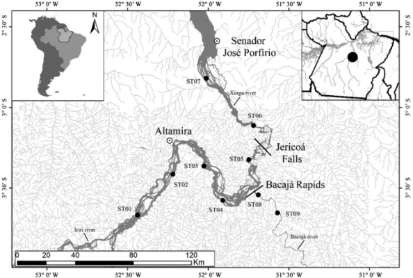
The Xingu River is a major right-bank tributary of the Amazon River, which originates in the Brazilian state of Mato Grosso, in the Serra do Roncador region, and discharges into the Amazon just downstream from the town of Porto de Moz, in Pará state. The river is 2,045 km long and flows predominantly in a south-north direction. Its principal tributary is the Iriri River, which originates approximately 100 km to the southwest of the town of Altamira, and other important tributaries of Xingu river are the Bacajá and Bacajaí rivers, on the Volta Grande do Xingu, downstream from Altamira (Eletronorte, 2001; Salomão et al., 2007; Eletrobras, 2009; Castilhos and Buckup, 2011).
The climate of this region is Am in the Köppen-Geiger classification, that is, tropical hot and humid (Peel et al., 2007). During the study period, monthly rainfall varied from 10.8 mm to 478.3 mm (INMET, 2014) and between 1971 and 2013, flow ranged from 1142.53 m3/s to 19518.23 m3/s on average, creating four distinct hydrological periods: Receding Water (June-August), Low Water (September-November), Flooding (December and February), and High Water (March-May). Because of this variation in river level, reaching on average 4.8 m in High Water period (Goulding et al., 2003), different environments become available during the year, including floodplains and flooded forests. In addition, some streams and lakes that connect with the river in High Water become isolated during the Low Water season.
03°23’24.9” S and 051°43’55.9” W; known as Jericoá, it presents a fairly sharp waterfall, where only large migratory fish can pass through. In addition, rapids in Bacajá River (a tributary of Xingu River) can be barriers too.
The present study focused on the middle Xingu, between the mouth of the Iriri River (20 km upstream of Altamira city) and the town of Senador José Porfírio (Figure 1). Data were collected tri-monthly between July 2012 and April 2013. In total, 36 sites were sampled, 9 in each hydrological period. Each sampling site was approximately 40 km, in fluvial distance, from each other.
2.2. Collection of biological samples and environmental data
Fish specimens were collected using a sequential set of gillnets with meshes of different sizes, with each set being referred to as a “battery”. Each battery was composed of seven, 20 m-long rectangular nets of 2 m in height made of monofilament nylon, with diagonal stretch meshes of 2, 4, 7, 10, 12, 15, and 18 cm. Each net had an area of 40 m2, with a total area of 280 m2 or 0.00028 km2 per battery.
The flood period is characterised by the availability of new habitats, such as swamps and floodplain lakes. Due to the presence of these environments, sampling effort increased during this period, including one battery per swamp or floodplain lake sampled. Thus, the data were standardised using a Capture Per Unit Effort (CPUE), where the abundance of each species during a given month was divided by the area of the batteries set at the site in
that month, providing a metric in the form of a number of individuals per km2 of net per hour (ind./km2/h). In other words, the CPUE was used as an index of species relative abundance, defined as the number of individuals captured per km2 of gillnet per hour.
Three batteries were set at each site, with a distance of at least 5 km between each battery, in order to avoid problems of spatial autocorrelation. All the nets remained in the water for 15 hours, between 5 pm and 8 am of the following morning. The set of three batteries at each site was considered a single sample. Total sampling effort for each period of the hydrological cycle was 88.2 km2 at High Water, 52.92 km2 during the Receding Water, 52.92 km2 at Low Water, and 48.51 km2 during the Flooding period. The difference in sampling effort was due to amount of habitat, such as flooded forests, which are available only at High Water.
Once collected, the specimens were identified to the lowest possible taxonomic level (to species in most cases), fixed in 10% formaldehyde for 48 hours, and conserved in 70% ethanol. All specimens were deposited in the ichthyological collection at the Laboratório de Ictiologia de Altamira (LIA) of Universidade Federal do Pará (UFPA), as well as in the Museu Paraense Emílio Goeldi (MPEG) in Belém (Pará, Brazil).
In addition to the biological data, a number of environmental variables were obtained from the Norte Energia database, derived from samples collected by the International Ecology Institute (IIEGA). These data
were collected near the sites of fish sampling. A total of 17 variables were analysed: alkalinity (acronym: Alk, unit: mg-CaCO3/L), total carbon (C, mg/g sed), chlorophyll a (cloa, µg/L), conductivity (cond, mS/cm), Biochemical Demand for Oxygen (BDO, mg/L), suspended organic matter (SOM, mg/L), suspended inorganic matter (SIM, mg/L), total suspended matter (TSM, mg/L), total nitrogen (N, mg/L), dissolved oxygen (DO, mg/L), pH, redox potential (redox, mV), depth (depth, m), total dissolved solids (DisSol, mg/L), temperature (temp, °C), transparency (transp, m), and turbidity (turb, UNT).
2.3. Data analysis
A Pearson Correlation Analysis was used to examine multicollinearity between variables, excluding those with correlation above a threshold of 0.8. A Principal Components Analysis (PCA) was used to determine which environmental variables were important in the differentiation of sites (Jongman, 1995). The axes were selected using the Broken Stick criterion. The environmental variables selected through this method were used for subsequent analyses. Prior to these analyses, the environmental variables were standardised by subtracting each value from the mean and then dividing it by the standard deviation in order to remove the effects of the different scales of measurement.
The pairwise distance between sites was measured following the course of the river, using 1:100,000 scale shape files of the local hydrography. To evaluate longitudinal variation in fish assemblage composition, the CPUE data (ind/km2/h) from each site were ordinated distances (Clarke and Warwick, 2001). After NMDS, data were tested using a Permutational Analysis of Variance (PERMANOVA) with sums of squares type III (partial), permutation of residuals under a reduced model and 999 permutations. The PERMANOVA was based on the null hypothesis that the composition of the fish assemblages did not vary significantly among hydrological periods and spatially. Lastly, an Indicator Species Analysis (IndVal) was run to investigate which species were responsible for the differences among sites and/or hydrological periods (Clarke and Warwick, 2001).
We used Mantel analysis to evaluate the correlation of four matrices with fish assemblage composition (environmental variables, hydrological periods, presence of waterfalls/rapids, and fluvial distance between points), based on Pearson’s correlation coefficient. We also tested the correlation among these four matrices with Mantel. When it was significant, we used partial Mantel to control the effect of each explanatory matrix on fish assemblages. Partial Mantel determines the partial correlation of two distance matrices, while controlling the effect of a third matrix (Legendre and Legendre, 2012), which allows us to see the individual effect of each matrix on the response matrix.
The matrix for the analysis of the hydrological periods was based on the pairwise comparison of sites by sample period. A score of zero was applied to pairs of samples from the same period (e.g., Flooding-Flooding), 1 for adjacent periods (e.g., Flooding-High Water), and 2 for alternate periods (e.g., Flooding-Receding Water). The matrix for
the presence of waterfalls or rapids was also based on pairs of sites, which were scored zero for the absence of barriers and 1 when a barrier existed between them.
All statistical analyses were run in the R program (R Development Core Team, 2011) using the Vegan (Oksanen et al., 2011) and Ecodist packages (Goslee and Urban, 2007). All tests considered a 5% significance level.
3. Results
3.1. Environmental variables
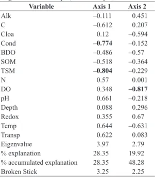
The High Water period was characterised by the highest alkalinity, BDO, depth, and redox potential. The highest temperatures and dissolved oxygen concentrations were recorded at Low Water. The highest values for all other variables were recorded during the transitional periods, that is, the Flooding and Receding Water cycles (see Appendix 1). The variables total dissolved solids and turbidity were excluded of the analysis because presented large correlation with conductivity. The same occurred with suspended inorganic matter that was correlated to total suspended matter. The first PCA axis explained 28.35% of the variation, and the second, 19.92%, with a total of 48.28% for the first two ordination axes (Table 1). The most important variables of the first axis (loading > 0.7) were conductivity and total suspended matter, both negatively associated with the first Principal Component. Dissolved oxygen was the variable that contributed most to the
Table 1. Results of the Principal Components Analysis (PCA) for the nine sample points surveyed on the middle Xingu River between April, 2012 and April, 2013.
Variable Axis 1 Axis 2
Alk –0.111 0.451
C –0.612 0.207
Cloa 0.12 –0.594
Cond –0.774 –0.152
BDO –0.486 –0.57
SOM –0.518 –0.364
TSM –0.804 –0.229
N 0.57 0.001
DO 0.348 –0.817
pH 0.661 –0.218
Depth 0.088 0.296
Redox 0.355 0.67
Temp 0.644 –0.631
Transp 0.622 0.083
Eigenvalue 3.97 2.79
% explanation 28.35 19.92
% accumulated explanation 28.35 48.28
Broken Stick 3.25 2.25
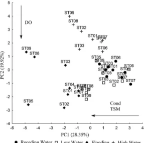
formation of axis 2 (Table 1), with a negative association. The plot (Figure 2) shows a clear grouping of the Receding Water and Low Water periods, characterised by increased dissolved oxygen and reduced conductivity and total suspended matter. The Flooding and High Water periods presented the opposite values, with increased values of conductivity and total suspended matter and reduced dissolved oxygen. The points showed no spatial pattern,
meaning that environmental variables did not group per sampling site.
3.2. Fish assemblages
A total of 8,485 fish specimens were collected during the present study, representing 188 species belonging to 33 families in nine orders (See Appendix 2). The most abundant order was Characiformes (5,765 specimens; 1,354.44 ind/km2/h of net), followed by Siluriformes (2,803; 678.65 ind/km2/h), and Perciformes (444; 104.91 ind/km2/h). The most abundant family was Hemiodontidae (1,424; 333.48 ind/km2/h), followed by Curimatidae (1,095; 261.97 ind/km2/h), and Characidae (1,144; 254.97 ind/km2/h). The most common species was Hemiodus unimaculatus (Bloch, 1794) (780; 185.87 ind/km2/h), then Ageneiosus ucayalensis Castelnau, 1855 (396; 70.56 ind/km2/h), and Tocantinsia
piresi (Miranda Ribeiro, 1920) (387; 56.69 ind/km2/h). The PERMANOVA indicated significant temporal variation in the characteristics of the fish fauna (pseudo-F = 3.45; d.f. = 3; p = 0.001), despite a certain degree of overlap between the Flooding and High Water period, as shown in the NMDS plot (Figure 3). Significant spatial differentiation was also observed (pseudo-F = 2.32; d.f. = 8; p = 0.001). After the PERMANOVA, it was possible to realize the formation of three groups, the first encompassing sites 8 and 9 (group 1), the second, sites 1 through 5 (group 2), and the third by sites 6 and 7, forming group 3 (Figure 3). Groups 1 and 2 were separated by the Bacajá rapids and groups 2 and 3 were separated by the Jericoá falls.
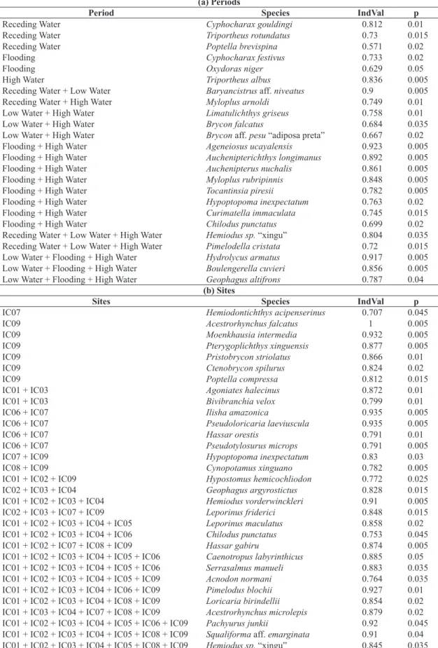
Different species contributed to the formation of the spatial groups and to the differentiation among hydrological periods (Table 2). The IndVal test selected 31 species with
Figure 2. Plot of the PCA for the hydrological periods and sample sites surveyed on the middle Xingu River between July, 2012, and April, 2013.
Table 2. Results of Indicator Species Analysis per hydrologic period (a) and per sampling site (b) of the fish assemblages on the middle Xingu River.
(a) Periods
Period Species IndVal p
Receding Water Cyphocharax gouldingi 0.812 0.01
Receding Water Triportheus rotundatus 0.73 0.015
Receding Water Poptella brevispina 0.571 0.02
Flooding Cyphocharax festivus 0.733 0.02
Flooding Oxydoras niger 0.629 0.05
High Water Triportheus albus 0.836 0.005
Receding Water + Low Water Baryancistrus aff. niveatus 0.9 0.005
Receding Water + High Water Myloplus arnoldi 0.749 0.01
Low Water + High Water Limatulichthys griseus 0.758 0.01
Low Water + High Water Brycon falcatus 0.684 0.035
Low Water + High Water Brycon aff. pesu “adiposa preta” 0.667 0.02
Flooding + High Water Ageneiosus ucayalensis 0.923 0.005
Flooding + High Water Auchenipterichthys longimanus 0.892 0.005
Flooding + High Water Auchenipterus nuchalis 0.861 0.005
Flooding + High Water Myloplus rubripinnis 0.848 0.005
Flooding + High Water Tocantinsia piresii 0.782 0.005
Flooding + High Water Hypoptopoma inexpectatum 0.763 0.02
Flooding + High Water Curimatella immaculata 0.745 0.015
Flooding + High Water Chilodus punctatus 0.699 0.02
Receding Water + Low Water + High Water Hemiodus sp. “xingu” 0.804 0.035
Receding Water + Low Water + High Water Pimelodella cristata 0.72 0.015
Low Water + Flooding + High Water Hydrolycus armatus 0.917 0.005
Low Water + Flooding + High Water Boulengerella cuvieri 0.856 0.005
Low Water + Flooding + High Water Geophagus altifrons 0.787 0.04
(b) Sites
Sites Species IndVal p
IC07 Hemiodontichthys acipenserinus 0.707 0.045
IC09 Acestrorhynchus falcatus 1 0.005
IC09 Moenkhausia intermedia 0.932 0.005
IC09 Pterygoplichthys xinguensis 0.877 0.005
IC09 Pristobrycon striolatus 0.866 0.01
IC09 Ctenobrycon spilurus 0.824 0.02
IC09 Poptella compressa 0.812 0.015
IC01 + IC03 Agoniates halecinus 0.872 0.01
IC01 + IC03 Bivibranchia velox 0.799 0.01
IC06 + IC07 Ilisha amazonica 0.935 0.005
IC06 + IC07 Pseudoloricaria laeviuscula 0.935 0.005
IC06 + IC07 Hassar orestis 0.791 0.01
IC06 + IC07 Pseudotylosurus microps 0.791 0.005
IC07 + IC09 Hypoptopoma inexpectatum 0.83 0.03
IC08 + IC09 Cynopotamus xinguano 0.782 0.005
IC01 + IC02 + IC09 Hypostomus hemicochliodon 0.772 0.025
IC02 + IC03 + IC04 Geophagus argyrostictus 0.828 0.015
IC01 + IC02 + IC03 + IC04 Hemiodus vorderwinckleri 0.91 0.005
IC02 + IC03 + IC07 + IC09 Leporinus friderici 0.848 0.015
IC01 + IC02 + IC03 + IC04 + IC05 Leporinus maculatus 0.858 0.02
IC01 + IC02 + IC03 + IC04 + IC06 Chilodus punctatus 0.753 0.045
IC01 + IC02 + IC07 + IC08 + IC09 Hassar gabiru 0.874 0.005
IC01 + IC02 + IC03 + IC04 + IC05 + IC06 Caenotropus labyrinthicus 0.885 0.05
IC01 + IC02 + IC03 + IC04 + IC05 + IC06 Serrasalmus manueli 0.883 0.035
IC01 + IC02 + IC03 + IC04 + IC05 + IC09 Acnodon normani 0.764 0.035
IC01 + IC02 + IC03 + IC04 + IC06 + IC09 Pimelodus blochii 0.927 0.01
IC01 + IC02 + IC03 + IC04 + IC08 + IC09 Loricaria birindellii 0.854 0.02
IC01 + IC03 + IC04 + IC07 + IC08 + IC09 Acestrorhynchus microlepis 0.879 0.02
IC01 + IC02 + IC03 + IC04 + IC05 + IC06 + IC09 Pachyurus junkii 0.92 0.045
occurrence linked to the sampling sites, while 24 species were related to hydrological periods.
3.3. Factors that affect the distribution of fish species
The Mantel analysis between the four explanatory matrices indicated a very weak correlation between the environmental variables and the hydrological periods, so this correlation was not considered in this study, although it was statistically significant (Table 3). On the other hand, there was a strong correlation between the presence of barriers and the fluvial distance. The effect of each matrix was then analysed separately to see their effects on fish assemblages.
The Mantel analysis indicated that the explanatory variables were responsible for 62% of the variation in the data (Table 3). Only the hydrological period and the presence of barriers (waterfalls or rapids) affected the distribution of the fish fauna, with the latter (barriers) being the most important. There was no influence of distance between sample points neither of environmental variables on fish assemblages.
4. Discussion
The hydrological cycle (temporal effect) and the presence of waterfalls (structural effect) are the main determinants of the fish species distribution in the middle Xingu River, confirming predictions iii and iv. Habitat connectivity among hydrologic periods is the main factor regulating the dispersal of individuals to new areas and to access new resources. In the case of lotic ecosystems, connectivity is observed longitudinally in relation to the course of the river, and laterally in relation to the influence of the hydrological cycle (Kondolf et al., 2006), with the formation of a vast flood plain.
Rivers and streams are dynamic and complex systems with a unidirectional flow of matter and energy. These processes modify gradually environmental conditions
and the distribution of resources exploited by fishes, these variations being explained by the River Wave Theory (Humphries et al., 2014). This results in variations in the structure of fish assemblages along a longitudinal gradient, although the continuity of this gradient, the autochthonous production or allochthonous inputs. These factors may be interrupted abruptly and modified by the presence of physical barriers, such as waterfalls and rapids, resulting in distinct assemblages on either side of the barrier (Agostinho et al., 2008; Torrente-Vilara et al., 2011). Our study confirms this, since we observed the formation of groups between the waterfalls.
The characteristics of Neotropical fish assemblages also vary considerably in relation to the fluctuations caused by the seasonal flood pulse (Goulding, 1980; Junk et al., 1989; Scarabotti et al., 2011; Silva et al., 2013; Humphries et al., 2014). This process results in the inundation of the floodplain swamps, expanding the availability of resources (food and refuges, for example) and increasing the connectivity among habitats, resulting in a random redistribution of the fish fauna and reducing spatial variability (Thomaz et al., 2007). As the water drains back into the main channel, nutrients are washed out, while fish density and biotic interactions increase, some environments being isolated (Goulding, 1980; Junk et al., 1989). In the present study, the composition of the assemblages was affected by hydrologic periods, varying significantly among seasons, as recorded in a number of previous studies in the Neotropical region (Scarabotti et al., 2011; Silva et al., 2013). However, the effects of the Jericoá falls and Bacajá rapids were more pronounced than those of the flood pulse, and represent a major factor in the structuring of the fish assemblages of the middle Xingu. A similar pattern has been recorded in a number of previous studies of the effects of natural barriers on the abundance and distribution of fish species (Ingênito and Buckup, 2007; Torrente-Vilara et al., 2011).
Given the importance of physical barriers such as waterfalls and the habitat connectivity caused by the annual flood pulse, the construction of hydroelectric dams may have a significant impact on the composition of fish assemblages. In the specific case of the Belo Monte project on the Xingu River, which is being constructed in the middle of the study area, there is a predicted reduction in river discharge on the stretch that includes the Jericoá falls (Eletronorte, 2001; Norte Energia, 2010). This would result in the permanent loss of connectivity between the fish assemblages located up- and down-stream of these falls, as well as a marked change in the types of habitat available for the different species, which would affect species composition, as well as reproductive patterns and the recruitment processes of the majority of taxa (Agostinho et al., 2004). The impacts of the construction of hydroelectric dams are well documented (Junk and Mello, 1990; Agostinho et al., 2008; Mims and Olden, 2013; Sakaris, 2013; Freedman et al., 2014) and are related primarily to processes such as the loss and homogenization of habitats, and the replacement of species. This emphasizes the need for the systematic collection of data on the characteristics of local fish assemblages prior Table 3. Results of the Mantel analysis between the four
explanatory matrices ̶ environmental variables, hydrological periods, the presence of barriers (waterfalls or rapids), and fluvial distance between points ̶ and their effects on the composition of the fish assemblages on the middle Xingu River.
R p
Environment x Period 0.07 0.01
Environment x Waterfall –0.05 0.78
Environment x Fluvial distance –0.10 0.91
Period x Waterfall –0.05 1
Period x Fluvial distance –0.06 1
to the flooding of reservoirs, in order to provide a sound database for the development of effective management strategies. However, little is known about the effect of the construction of reduced flow hydroelectric dams and this knowledge is nil when it comes to Amazon. Thus, this study is important because it allows the understanding of the structure of fish populations in the Middle Xingu River, forming bases for possible conservation measures.
The results of the present study indicated that the presence of waterfalls and the fluctuations of the flood pulse were the primary factors determining the distribution of fish species within the study area, creating both longitudinal and lateral gradients. This supports two of the operational hypotheses tested in the study, but rejects those on the possible effects of local environmental variables or the distance between sites. The difference in the composition of the assemblies due to hydrological periods and physical barriers are clearly the most important determinants of the structure of ichthyofauna in the study area, and is also one of the characteristics that may be most impacted by the construction of the Belo Monte hydroelectric dam. This re-emphasizes the need for the consideration of the region’s unique characteristics in the planning of future management strategies.
Acknowledgements
This research was supported by Norte Energia and LEME. The collection of biological material was authorised by permit 057/2012 from IBAMA, the Brazilian Institute for the Environment and renewable Natural Resources. TAPB and NLB were funded by CNPq, and TG (process: 308278/2012-7), LJ (process: 303252/2013-8) and LFAM (process: 301343/2012-8) receive productivity grants from CNPq. We are grateful to Dr. Stephen Ferrari for his help in correcting the text, particularly with the translation to English. All authors belong to the IctioXingu CNPq Research Group.
References
AGOSTINHO, AA., GOMES, LC., VERÍSSIMO, S. and OKADA, EK., 2004. Flood regime, dam regulation and fish in the Upper Paraná River: effects on assemblage attributes, reproduction and recruitment. Reviews in Fish Biology and Fisheries, vol. 14, no. 1, p. 11-19. http://dx.doi.org/10.1007/s11160-004-3551-y.
AGOSTINHO, AA., PELICICE, FM. and GOMES, LC., 2008. Dams and the fish fauna of the Neotropical Region: impacts and management related to diversity and fisheries. Brazilian Journal of Biology, vol. 68, no. 4, supplement, p. 1119-1132. http://dx.doi. org/10.1590/S1519-69842008000500019. PMid:19197482.
CASTILHOS, ZC. and BUCKUP, PA., 2011. Ecorregião aquática Xingu-Tapajós. Rio de Janeiro: CETEM/MCT. 248 p. CLARKE, KR. and WARWICK, RW., 2001. Change in marine communities: an approach to statistical analysis and interpretation. Reino Unido: Plymouth Marine Laboratory. 859 p.
Eletrobras, 2009. Aproveitamento hidrelétrico Belo Monte - Relatório de Impacto Ambiental - Rima. Brasília: Ministério de Minas e Energia. 100 p.
Eletronorte, 2001. Complexo hidrelétrico de Belo Monte. Estudo de impacto ambiental. Brasília: Eletronorte. 32 p. Mimeo FREEDMAN, JA., LORSON, BD., TAYLOR, RB., CARLINE, RF. and STAUFFER JUNIOR, JR., 2014. River of the dammed: longitudinal changes in fish assemblages in response to dams. Hydrobiologia, vol. 727, no. 1, p. 19-33. http://dx.doi.org/10.1007/ s10750-013-1780-6.
GOSLEE, SC. and URBAN, DL., 2007. The ecodist package for dissimilarity-based analysis of ecological data. Journal of Statistical Software, vol. 22, no. 7, p. 1-19.
GOULDING, M., 1980. The fishes and the forest: explorations in Amazonian natural history. London: University of California Press. 280 p.
GOULDING, M., BARTHEM, R. and FERREIRA, EJG., 2003. The Smithsonian atlas of the Amazon. Washington: Smithsonian Books. 253 p.
HOEINGHAUS, DJ., WINEMILLER, KO. and BIRNBAUM, JS., 2007. Local and regional determinants of stream fish assemblage structure: inferences based on taxonomic vs. functional groups. Journal of Biogeography, vol. 34, no. 2, p. 324-338. http://dx.doi. org/10.1111/j.1365-2699.2006.01587.x.
HUBBELL, SP., 2001. The unified neutral theory of biodiversity and biogeography. West Sussex: Princeton University Press. 396 p.
HUMPHRIES, P., KECKEIS, H. and FINLAYSON, B., 2014. The river wave concept: integrating river ecosystem models. Bioscience, vol. 64, no. 10, p. 870-882. http://dx.doi.org/10.1093/ biosci/biu130.
HUTCHINSON, GE., 1957. Population studies: animal ecology and demography - concluding remarks. Cold Spring Harbor Symposia on Quantitative Biology, vol. 22, p. 415-427. http:// dx.doi.org/10.1101/SQB.1957.022.01.039.
INGENITO, LFS. and BUCKUP, PA., 2007. The Serra da Mantiqueira, south-eastern Brazil, as a biogeographical barrier for fishes. Journal of Biogeography, vol. 34, no. 7, p. 1173-1182. http://dx.doi.org/10.1111/j.1365-2699.2007.01686.x.
Instituto Nacional de Meteorologia – INMET, 2014. Banco de dados meteorológicos para ensino e pesquisa. Available from: <http://www.inmet.gov.br/portal/index.php?r=bdmep/bdmep>. Access in: 7 Apr. 2014.
JONGMAN, RHG., 1995. Data analysis in community and landscape ecology. New York: Cambridge University Press. 321 p. http://dx.doi.org/10.1017/CBO9780511525575.
JUNK, WJ. and MELLO, JASN., 1990. Impactos ecológicos das represas hidrelétricas na bacia amazônica brasileira. Estudos Avançados, vol. 4, no. 8, p. 126-143. http://dx.doi.org/10.1590/ S0103-40141990000100010.
JUNK, WJ., 1980. Áreas inundáveis: um desafio para a limnologia. Acta Amazonica, vol. 10, no. 4, p. 775-796.
JUNK, WJ., BAYLEY, PB. and SPARKS, RE., 1989. The flood pulse concept in river-floodplain systems. In DODGE, DP. (Ed.). Proceedings of the International Large River Symposium, 1990. Quebec: Canadian Government Publishing Centre. p. 110-127. Canadian Special Publication of Fisheries and Aquatic Sciences, 106.
dynamic vectors to recover lost linkages. Ecology and society, vol. 11, no. 2, p. 1-17.
LEGENDRE, P. and LEGENDRE, L., 2012. Numerical ecology. Amsterdam: Elsevier Science BV. 1006 p.
MARQUES, PHC., OLIVEIRA, HTD. and MACHADO, EDC., 2003. Limnological study of Piraquara river (Upper Iguaçu Basin): spatiotemporal variation of physical and chemical variables and watershed zoning. Brazilian Archives of Biology and Technology, vol. 46, no. 3, p. 383-394. http://dx.doi.org/10.1590/S1516-89132003000300010.
MIMS, MC. and OLDEN, JD., 2013. Fish assemblages respond to altered flow regimes via ecological filtering of life history strategies. Freshwater Biology, vol. 58, no. 1, p. 50-62. MORLON, H., CHUYONG, G., CONDIT, R., HUBBELL, S., KENFACK, D., THOMAS, D., VALENCIA, R. and GREEN, JL., 2008. A general framework for the distance-decay of similarity in ecological communities. Ecology Letters, vol. 11, no. 9, p. 904-917. http://dx.doi.org/10.1111/j.1461-0248.2008.01202.x. PMid:18494792.
NEKOLA, JC. and WHITE, PS., 1999. Special paper: the distance decay of similarity in biogeography and ecology. Journal of Biogeography, vol. 26, no. 4, p. 867-878. http://dx.doi. org/10.1046/j.1365-2699.1999.00305.x.
Norte Energia, 2010. Plano Básico Ambiental (PBA). Available from: <http://philip.inpa.gov.br/publ_livres/Dossie/BM/DocsOf/ PBA/Projeto%20B%C3%A1sico%20Ambiental-PBA.htm>. Access in: 10 Mar. 2013.
OKSANEN, J., BLANCHET, FG., KINDT, R., LEGENDRE, P., MINCHIN, PR. and O’HARA, RB., 2011. Vegan: Community Ecology Package. R package version 2.0-2. CRAN. 282 p.
PEEL, MC., FINLAYSON, BL. and MCMAHON, TA., 2007. Updated world map of the Köppen-Geiger climate classification. Hydrology and Earth System Sciences, vol. 11, no. 5, p. 1633-1644. http://dx.doi.org/10.5194/hess-11-1633-2007.
R Development Core Team, 2011. R: A Language and Environment for Statistical Computing. Vienna: R Foundation for Statistical Computing. Available from: <http://www.R-project.org>. Access in: 10 Mar. 2013.
RODRÍGUEZ, MA. and LEWIS JUNIOR, WM., 1994. Regulation and stability in fish assemblages of neotropical floodplain lakes.
Oecologia, vol. 99, no. 1-2, p. 166-180. http://dx.doi.org/10.1007/ BF00317098.
SAKARIS, PC., 2013. A review of the effects of hydrologic alteration on fisheries and biodiversity and the management and conservation of natural resources in regulated river systems: current perspectives in contaminant hydrology and water resources sustainability. Croatia: InTech. p. 273-297. http://dx.doi. org/10.5772/55963. Available from: <http://www.intechopen.com/ books/current-perspectives-in-contaminant-hydrology-and-water- resources-sustainability/a-review-of-the-effects-of-hydrologic-alteration-on-fisheries-and-biodiversity-and-the-management-an>. Access in: 10 Mar. 2013.
SALOMÃO, RP., VIEIRA, ICG., SUEMITSU, C., ROSA, NA., ALMEIDA, SS., AMARAL, DD. and MENEZES, MPM., 2007. As florestas de Belo Monte na grande curva do rio Xingu, Amazônia oriental. Boletim do Museu Paraense Emílio Goeldi. Ciências Naturais, vol. 2, no. 3, p. 57-153.
SCARABOTTI, PA., LÓPEZ, JA. and POUILLY, M., 2011. Flood pulse and the dynamics of fish assemblage structure from neotropical floodplain lakes. Ecology Freshwater Fish, vol. 20, no. 4, p. 605-618. http://dx.doi.org/10.1111/j.1600-0633.2011.00510.x.
SILVA, MT., PEREIRA, JO., VIEIRA, LJS. and PETRY, AC., 2013. Hydrological seasonality of the river affecting fish community structure of oxbow lakes: a limnological approach on the Amapá Lake, southwestern Amazon. Limnologica, vol. 43, no. 2, p. 79-90. http://dx.doi.org/10.1016/j.limno.2012.05.002.
SOUTHWOOD, TRE., 1977. Habitat, the templet for ecological strategies. Journal of Animal Ecology, vol. 46, no. 2, p. 337-365. http://dx.doi.org/10.2307/3817.
SUAREZ, YR. and PETRERE-JUNIOR, M., 2007. Environmental factors predicting fish community structure in two neotropical rivers in Brazil. Neotropical Ichthyology, vol. 5, no. 1, p. 61-68. http://dx.doi.org/10.1590/S1679-62252007000100008.
THOMAZ, SM., BINI, LM. and BOZELLI, RL., 2007. Floods increase similarity among aquatic habitats in river-floodplain systems. Hydrobiologia, vol. 579, no. 1, p. 1-13. http://dx.doi. org/10.1007/s10750-006-0285-y.
87
Fish assemblages of the middle Xingu River
87
low water, flood, and high water) between July, 2012, and April, 2013. Alk = Alkalinity (mg-CaCO3/L), C = Total carbon (mg/g sed), Cloa = Chlorophyll a (µg/L), Cond = Condutivity (mS/cm), BDO = Biochemical Demand for Oxygen (mg/L), SIM = Suspended Inorganic Matter (mg/L), SOM = Suspended Organic Matter (mg/L), TSM = Total Suspended Matter (mg/L), N = Total nitrogen (mg/L), DO = Dissolved oxygen (mg/L), pH, Depth = depth (m), Redox = Redox potential (mV), SolDiss = Total Dissolved Solids (mg/L), Temp = Temperature (°C), Transp = Transparency (m), and Turb = Turbidity (UNT).
Period Alk C Cloa Cond BDO SIM SOM TSM N DO pH Depth Redox SolDiss Temp Transp Turb
Receding Water 6.59±
3.16 0.27± 0.16 12.92± 5.82 0.02± 0.001 0.67± 0.28 3.82± 2.34 2.31± 0.55 6.13± 2.71 2.76± 5.74 7.12± 0.26 7.98± 0.30 3.16± 5.21 117.23± 14.09 0.01± 0.01 29.85± 0.68 1.06± 0.32 4.60± 2.44
Low water 7.36±
5.73 6.96± 5.96 4.87± 3.18 0.02± 0.02 1.05± 0.60 4.57± 6.21 2.58± 1.60 7.14± 7.70 0.87± 0.50 7.54± 0.22 7.47± 0.60 2.02± 4.28 77.94± 28.04 0.01± 0.01 30.85± 0.61 0.81± 0.71 5.02± 5.19 Flooding 7.05± 6.28 7.71± 6.53 7.56± 4.55 0.03± 0.02 0.77± 0.40 2.93± 6.01 2.99± 2.15 5.92± 7.98 0.44± 0.11 7.37± 0.77 7.89± 0.79 2.12± 3.60 116.42± 28.67 0.01± 0.01 31.24± 0.36 0.92± 0.86 6.43± 5.44
High water 5.00±
Appendix 2. Taxonomic list of the fish species collected during the present study and their respective CPUE (ind./km2/h) for each hydrological period between July/2012 and April/2013 (Laboratório de Ictiologia de Altamira - LIA and Museu Paraense Emílio Goeldi - MPEG).
Taxon / Authority Voucher
High
Water
(ind./ km2/h)
Flooding
(ind./ km2/h)
Low Water
(ind./ km2/h)
Receding
Water
(ind./ km2/h)
Total
(ind./ km2/h) BELONIFORMES
Belonidae
Pseudotylosurus microps (Günther, 1866) LIA 404 3.741 2.721 0.000 0.227 6.689 CHARACIFORMES
Acestrorhynchidae
Acestrorhynchus falcatus (Bloch, 1794) MPEG 29909 6.198 0.454 1.361 4.308 12.320
Acestrorhynchus microlepis (Jardine, 1841) MPEG
28903 22.751 15.420 8.503 7.370 54.044
Anostomidae
Anostomoides passionis Santos & Zuanon,
2006 LIA 417 0.227 0.227 0.000 0.000 0.454
Hypomasticus julii (Santos, Jégu & Lima,
1996) MPEG 29314 2.494 0.227 0.000 2.041 4.762
Laemolyta fernandezi Myers, 1950 MPEG
29078 0.454 0.227 0.000 0.000 0.680
Laemolyta proxima (Garman, 1890) LIA 161 6.311 5.442 0.680 0.000 12.434
Leporinus aff. fasciatus LIA 134 15.004 2.041 3.061 8.277 28.328
Leporinus brunneus Myers, 1950 LIA 418 0.454 0.000 0.000 0.227 0.680
Leporinus desmotes Fowler, 1914 LIA 313 1.663 0.000 1.701 0.113 3.477
Leporinus friderici (Bloch, 1794) MPEG
28073 10.204 2.721 2.834 3.515 19.274
Leporinus maculatus Müller & Troschel,
1844 LIA 370 12.207 3.628 2.154 4.082 22.071
Leporinus sp. 1 MPEG
28837 0.000 0.000 0.000 0.227 0.227
Leporinus sp. 2 MPEG
28938 0.756 0.000 0.227 0.000 0.983
Leporinus tigrinus Borodin, 1929 MPEG
28996 0.907 0.000 0.000 0.907 1.814
Petulanos intermedius (Winterbottom,
1980) MPEG 29626 0.529 0.227 0.000 0.000 0.756
Pseudanos trimaculatus (Kner, 1858) MPEG
29440 0.869 0.227 0.000 0.340 1.436
Sartor respectus Myers & Carvalho, 1959 MPEG
28924 0.227 0.000 0.227 0.000 0.454
Schizodon vittatus (Valenciennes, 1850) MPEG
29057 1.134 0.680 0.113 0.340 2.268
Synaptolaemus latofasciatus (Steindachner,
1910) 0.151 0.000 0.000 0.000 0.151
Characidae
Acestrocephalus stigmatus Menezes, 2006 MPEG
28849 0.302 0.000 0.113 0.000 0.416
Agoniates halecinus Müller & Troschel,
1845 LIA 409 4.460 2.721 1.701 3.741 12.623
Astyanax gr. bimaculatus LIA 419 0.756 0.000 0.000 0.680 1.436
Brycon sp. 1 LIA 203 5.518 1.361 1.927 1.134 9.939
Brycon sp. 2 LIA 420 2.230 0.000 1.020 0.000 3.250
Brycon falcatus Müller & Troschel, 1844 MPEG
Taxon / Authority Voucher
High
Water
(ind./ km2/h)
Flooding
(ind./ km2/h)
Low Water
(ind./ km2/h)
Receding
Water
(ind./ km2/h)
Total
(ind./ km2/h)
Bryconops alburnoides Kner, 1858 MPEG
28979 2.608 0.227 0.794 1.587 5.215
Bryconops caudomaculatus (Günther,
1864) MPEG 29003 0.227 0.227 0.000 0.000 0.453
Bryconops giacopinii (Fernández-Yépez,
1950) MPEG 29402 0.000 0.567 0.000 0.000 0.566
Chalceus epakros Zanata & Toledo-Piza,
2004 LIA 157 1.134 0.000 0.680 0.000 1.814
Charax gibbosus (Linnaeus, 1758) LIA 342 0.907 0.000 0.907 0.000 1.814
Ctenobrycon spilurus (Valenciennes, 1850) MPEG
29817 2.305 0.000 0.340 1.587 4.232
Cynopotamus xinguano Menezes, 2007 MPEG
29587 3.364 0.227 1.020 2.154 6.764
Jupiaba polylepis (Günther, 1864) MPEG
29017 1.020 0.907 0.113 0.000 2.040
Moenkhausia heikoi Géry & Zarske, 2004 MPEG
28982 6.274 4.762 0.227 0.000 11.262
Moenkhausia intermedia Eigenmann, 1908 MPEG
28844 36.168 16.440 9.524 11.451 73.582
Moenkhausia lepidura (Kner, 1858) MPEG
28867 0.567 0.227 0.000 0.340 1.133
Moenkhausia xinguensis (Steindachner,
1882) MPEG 28083 8.428 3.175 0.454 1.134 13.189
Poptella brevispina Reis, 1989 LIA 410 5.329 0.000 0.227 5.669 11.224
Poptella compressa (Günther, 1864) MPEG
29019 9.259 2.381 4.875 0.000 16.515
Roeboexodon guyanensis (Puyo, 1948) MPEG
29407 0.567 0.227 0.000 0.340 1.133
Roeboides sp. MPEG
28899 2.608 0.227 2.041 0.340 5.215
Tetragonopterus argenteus (Puyo, 1948) MPEG
29871 1.474 0.680 0.000 0.794 2.947
Tetragonopterus chalceus Spix & Agassiz, 1829
MPEG
28943 3.288 1.134 1.247 0.794 6.462
Triportheus albus Cope, 1872 MPEG
29112 19.048 5.556 0.000 1.361 25.963
Triportheus auritus (Valenciennes, 1850) MPEG
29631 4.649 0.680 0.000 4.535 9.863
Triportheus rotundatus (Jardine, 1841) MPEG
29352 10.280 1.587 0.000 9.864 21.730
Chilodontidae
Caenotropus labyrinthicus (Kner, 1858) MPEG
28838 27.211 4.308 6.009 15.646 53.174
Chilodus punctatus Müller & Troschel, 1844
MPEG
29059 15.684 10.091 2.041 1.814 29.629
Ctenoluciidae
Boulengerella cuvieri (Spix & Agassiz,
1829) MPEG 28070 13.568 6.689 4.082 0.227 24.565
Boulengerella maculata (Valenciennes, 1850) LIA 272 1.587 1.134 0.454 0.000 3.174 Curimatidae
Curimata inornata Vari, 1989 MPEG
28876 37.906 18.367 4.308 15.193 75.774
Taxon / Authority Voucher
High
Water
(ind./ km2/h)
Flooding
(ind./ km2/h)
Low Water
(ind./ km2/h)
Receding
Water
(ind./ km2/h)
Total
(ind./ km2/h)
Curimata vittata (Kner, 1858) LIA 421 0.907 0.907 0.000 0.000 1.814
Curimatella dorsalis (Eigenmann &
Eigenmann, 1889) MPEG 29838 1.512 0.000 0.907 0.000 2.418
Curimatella immaculata
(Fernández-Yépez, 1948) MPEG 29526 10.506 7.596 0.000 0.000 18.102
Cyphocharax festivus Vari, 1992 LIA 366 39.985 43.084 0.000 0.000 83.068
Cyphocharax gouldingi Vari, 1992 MPEG
28893 16.289 2.268 4.308 37.528 60.393
Cyphocharax leucostictus (Eigenmann &
Eigenmann, 1889) MPEG 29535 7.181 8.957 1.020 0.000 17.157
Cyphocharax stilbolepis Vari, 1992 LIA 367 2.230 0.454 0.000 0.000 2.683
Psectrogaster falcata (Eigenmann &
Eigenmann, 1889) LIA 308 0.340 0.227 0.000 0.000 0.566
Cynodontidae
Cynodon gibbus (Agassiz, 1829) MPEG 28908 2.683 0.454 0.340 1.134 4.610
Hydrolycus armatus (Jardine, 1841) LIA 401 10.242 2.948 3.855 0.227 17.271
Hydrolycus tatauaia Toledo-Piza, Menezes & Santos, 1999
MPEG
29086 3.477 0.907 1.134 0.680 6.198
Rhaphiodon vulpinus Spix & Agassiz, 1829 MPEG
29085 3.704 0.227 1.134 1.474 6.538
Erythrinidae
Hoplias aimara (Valenciennes, 1847) MPEG
29904 0.680 0.567 0.000 0.227 1.473
Hoplias malabaricus (Bloch, 1794) MPEG
28067 1.701 0.680 0.794 0.113 3.287
Hemiodontidae
Argonectes robertsi Langeani, 1999 MPEG
28961 21.958 10.431 2.608 1.814 36.810
Bivibranchia fowleri (Steindachner, 1908) MPEG
28883 5.102 1.814 4.195 0.000 11.111
Bivibranchia velox (Eigenmann & Myers,
1927) MPEG 29105 6.463 2.154 2.381 3.401 14.399
Hemiodus cf. semitaeniatus LIA 422 6.122 6.122 0.000 0.000 12.244
Hemiodus sp. 1 MPEG
29072 22.373 0.680 7.937 9.864 40.854
Hemiodus unimaculatus (Bloch, 1794) MPEG
28887 99.471 39.569 19.955 26.871 185.865
Hemiodus vorderwinckleri (Géry, 1964) LIA 371 16.667 7.256 2.268 6.009 32.199
Prochilodontidae
Prochilodus nigricans Spix & Agassiz,
1829 LIA 298 3.401 1.361 1.020 0.454 6.235
Semaprochilodus brama (Valenciennes,
1850) MPEG 28968 6.236 2.721 2.948 1.814 13.718
Serrasalmidae
Acnodon normani Gosline, 1951 LIA 181 4.611 1.927 2.608 0.113 9.259
Metynnis cf. luna LIA 423 4.157 2.494 0.454 1.134 8.238
Myleus setiger Müller & Troschel, 1844 LIA 413 3.099 0.907 1.701 0.454 6.160
Myloplus arnoldi (Ahl, 1936) MPEG
28966 6.387 0.454 0.567 5.669 13.076
Myloplus rhomboidalis (Cuvier, 1818) LIA397 2.948 1.134 0.907 0.907 5.895
Taxon / Authority Voucher
High
Water
(ind./ km2/h)
Flooding
(ind./ km2/h)
Low Water
(ind./ km2/h)
Receding
Water
(ind./ km2/h)
Total
(ind./ km2/h)
Myloplus rubripinnis (Müller & Troschel,
1844) LIA 374 11.300 3.741 2.494 0.000 17.535
Myloplus schomburgkii (Jardine, 1841) LIA163 2.494 0.227 1.361 0.794 4.875
Pristobrycon eigenmanni (Norman, 1929) LIA 297 0.227 0.000 0.227 0.000 0.453
Pristobrycon striolatus (Steindachner,
1908) LIA 411 3.401 1.587 1.247 0.567 6.802
Pygocentrus nattereri Kner, 1858 LIA 300 1.474 0.000 0.680 0.794 2.947
Serrasalmus altispinis Merckx, Jégu &
Santos, 2000 LIA 424 2.834 0.000 2.834 0.000 5.668
Serrasalmus gouldingi Fink & Machado-Allison, 1992
MPEG
28860 1.587 0.227 0.000 1.361 3.174
Serrasalmus manueli (Fernández-Yépez &
Ramírez, 1967) LIA 393 22.978 2.494 13.152 6.689 45.313
Serrasalmus rhombeus (Linnaeus, 1766) LIA 351 17.385 1.020 4.195 10.317 32.917
Tometes sp. LIA 59 2.948 0.907 0.567 0.794 5.215 CLUPEIFORMES
Engraulidae
Anchoviella sp. MPEG
28064 0.680 0.680 0.000 0.000 1.360
Lycengraulis batesii (Günther, 1868) LIA 360 0.907 0.454 0.000 0.454 1.814
Pristigasteridae
Ilisha amazonica (Miranda & Ribeiro,
1920) MPEG 28870 12.812 5.215 0.907 0.907 19.841
Pellona castelnaeana Valenciennes, 1847 LIA 425 0.794 0.000 0.227 0.227 1.247 GYMNOTIFORMES
Electrophoridae
Electrophorus electricus (Linnaeus, 1766) LIA 426 0.113 0.000 0.000 0.113 0.226 Gymnotidae
Gymnotus carapo Linnaeus, 1758 LIA 427 0.529 0.000 0.000 0.000 0.529 Hypopomidae
Steatogenys elegans (Steindachner, 1880) MPEG
29292 0.227 0.000 0.000 0.227 0.453
Rhamphichthyidae
Rhamphichthys drepanium Triques, 1999 LIA 428 0.416 0.227 0.113 0.000 0.755 Sternopygidae
Archolaemus janeae Vari, de Santana &
Wosiacki, 2012 MPEG 28896 4.308 0.000 1.701 2.494 8.503
Eigenmannia aff. trilineata MPEG
29595 0.076 0.000 0.000 0.000 0.075
MYLIOBATIFORMES Potamotrygonidae
Paratrygon aiereba (Müller & Henle,
1841) LIA 314 0.227 0.227 0.000 0.000 0.453
OSTEOGLOSSIFORMES
Osteoglossidae
Osteoglossum bicirrhosum (Cuvier, 1829) LIA 276 1.361 0.000 1.361 0.000 2.721 PERCIFORMES
Cichlidae
Aequidens michaeli Kullander, 1995 MPEG
28846 0.227 0.227 0.000 0.000 0.453
Taxon / Authority Voucher
High
Water
(ind./ km2/h)
Flooding
(ind./ km2/h)
Low Water
(ind./ km2/h)
Receding
Water
(ind./ km2/h)
Total
(ind./ km2/h)
Caquetaia spectabilis (Steindachner, 1875) MPEG
28840 0.454 0.227 0.000 0.113 0.793
Cichla melaniae Kullander & Ferreira,
2006 LIA 64 2.268 0.000 0.113 1.587 3.968
Cichla monoculus Agassiz, 1831 LIA 63 0.227 0.000 0.227 0.000 0.453
Crenicichla gr. saxatilis LIA 429 0.113 0.000 0.000 0.113 0.226
Crenicichla lugubris Heckel, 1840 MPEG 28959 0.227 0.000 0.113 0.340 0.680
Crenicichla sp. LIA 81 1.134 0.454 0.000 0.680 2.267
Geophagus altifrons Heckel, 1840 MPEG
28081 12.094 4.422 7.143 0.794 24.452
Geophagus argyrostictus Kullander, 1991 MPEG
28962 7.521 0.794 4.649 1.247 14.210
Retroculus xinguensis Gosse, 1971 MPEG
29203 1.020 0.227 0.567 0.567 2.380
Satanoperca sp. MPEG
29334 0.340 0.000 0.113 0.113 0.566
Teleocichla sp. LIA 5 0.227 0.000 0.227 0.000 0.453
Sciaenidae
Pachyurus junki Soares & Casatti, 2000 MPEG
28085 20.446 4.422 9.751 4.649 39.266
Plagioscion squamosissimus (Heckel,
1840) LIA 362 8.957 1.814 3.175 0.794 14.739
PLEURONECTIFORMES Achiridae
Hypoclinemus mentalis (Günther, 1862) MPEG
29117 0.000 0.000 0.113 0.000 0.113
SILURIFORMES Auchenipteridae
Ageneiosus inermis (Linnaeus, 1766) 4.308 2.608 0.454 0.227 7.596
Ageneiosus ucayalensis Castelnau, 1855 MPEG
29114 43.915 23.696 2.381 0.567 70.559
Auchenipterichthys longimanus (Günther,
1864) MPEG 28834 19.992 5.329 0.567 1.020 26.908
Auchenipterus nuchalis (Spix & Agassiz,
1829) LIA 383 63.492 22.789 1.247 0.794 88.321
Centromochlus heckelii (De Filippi, 1853) MPEG
28063 12.245 9.977 0.000 2.268 24.489
Centromochlus schultzi Rössel, 1962 MPEG
29752 0.454 0.567 0.000 0.113 1.133
Tatia intermedia (Steindachner, 1877) MPEG
28925 0.529 0.454 0.000 0.000 0.982
Tocantinsia piresi (Miranda Ribeiro, 1920) LIA 363 34.014 22.676 0.000 0.000 56.689
Trachelyopterus ceratophysus (Kner, 1858) LIA 339 0.454 0.000 0.000 0.000 0.453 Callichthyidae
Megalechis picta (Müller & Troschel, 1849) MPEG
29903 0.113 0.000 0.000 0.113 0.226
Cetopsidae
Cetopsis coecutiens (Lichtenstein, 1819) MPEG
28061 3.628 0.000 0.227 3.401 7.256
Taxon / Authority Voucher
High
Water
(ind./ km2/h)
Flooding
(ind./ km2/h)
Low Water
(ind./ km2/h)
Receding
Water
(ind./ km2/h)
Total
(ind./ km2/h)
Doradidae
Doras higuchii Sabaj Pérez & Birindelli, 2008
MPEG
29368 8.919 1.474 5.215 2.494 18.102
Hassar gabiru Birindelli, Fayal &
Wosiacki, 2011 MPEG 28965 17.952 5.669 7.596 2.268 33.484
Hassar orestis (Steindachner, 1875) MPEG
28871 21.542 6.803 0.000 14.286 42.630
Leptodoras hasemani (Steindachner, 1915) MPEG
29120 2.494 1.701 2.041 0.000 6.235
Leptodoras praelongus (Myers &
Weitzman, 1956) MPEG 29740 0.113 0.000 0.000 0.113 0.226
Megalodoras uranoscopus (Eigenmann &
Eigenmann, 1888) MPEG 28076 1.058 0.340 0.000 0.567 1.965
Nemadoras elongatus (Boulenger, 1898) LIA 430 0.227 0.227 0.000 0.000 0.453
Ossancora asterophysa Birindelli & Sabaj
Pérez, 2011 LIA 275 1.134 0.680 0.000 0.454 2.267
Oxydoras níger (Valenciennes, 1821) LIA 369 1.587 1.701 0.000 0.113 3.401
Platydoras armatulus (Valenciennes, 1840) MPEG
28062 2.343 0.907 0.454 0.567 4.270
Platydoras sp. LIA 139 4.119 2.494 0.000 0.454 7.067
Rhinodoras boehlkei Glodek, Whitmire & Orcés, 1976
MPEG
28857 0.454 0.454 0.000 0.000 0.907
Heptapteridae
Imparfinis aff. hasemani LIA 431 0.113 0.000 0.000 0.113 0.226
Pimelodella cristata (Müller & Troschel,
1849) MPEG 28892 4.535 0.000 2.154 2.154 8.843
Pimelodella sp. 1 MPEG
29481 0.567 0.000 0.000 0.000 0.567
Pimelodella sp. 2 MPEG
28969 0.113 0.000 0.000 0.113 0.226
Loricariidae
Ancistrus ranunculus Muller, Rapp
Py-Daniel & Zuanon, 1994 LIA 131 0.227 0.227 0.000 0.000 0.453
Ancistrus sp. 1 LIA 169 0.454 0.454 0.000 0.000 0.907
Ancistrus sp. 2 LIA 77 0.680 0.340 0.227 0.000 1.247
Baryancistrus aff. niveatus LIA 170 6.236 0.227 2.948 3.288 12.698
Baryancistrus chrysolomus Rapp Py-Daniel, Zuanon & Ribeiro de Oliveira, 2011
LIA 387 1.587 0.227 1.134 0.227 3.174
Baryancistrus xanthellus Rapp Py-Daniel,
Zuanon & Ribeiro de Oliveira, 2011 LIA 171 1.474 0.340 1.020 0.113 2.947
Hemiodontichthys acipenserinus (Kner,
1853) LIA 432 1.134 0.000 0.000 0.907 2.040
Hopliancistrus sp. LIA 433 0.227 0.227 0.000 0.000 0.454
Hypancistrus sp. LIA 21 0.227 0.000 0.227 0.000 0.453
Hypoptopoma inexpectatum (Holmberg,
1893) LIA 321 27.022 21.995 1.020 0.113 50.151
Hypostomus aff. plecostomus LIA 434 0.227 0.000 0.000 0.000 0.226
Hypostomus hemicochliodon Armbruster,
2003 LIA 359 2.041 0.454 0.680 0.340 3.514
Limatulichthys griseus (Eigenmann, 1909) LIA 380 5.556 0.454 2.268 0.000 8.276
Taxon / Authority Voucher
High
Water
(ind./ km2/h)
Flooding
(ind./ km2/h)
Low Water
(ind./ km2/h)
Receding
Water
(ind./ km2/h)
Total
(ind./ km2/h)
Loricaria birindellii Thomas & Sabaj
Pérez, 2010 LIA 85 8.163 2.268 2.041 4.989 17.460
Loricaria cataphracta Linnaeus, 1758 LIA 365 7.143 0.000 2.721 5.215 15.079
Panaque armbrusteri Lujan, Hidalgo &
Stewart, 2010 LIA 137 0.794 0.227 0.340 0.227 1.587
Parancistrus nudiventris Rapp Py-Daniel
& Zuanon, 2005 LIA 177 0.794 0.000 0.794 0.000 1.587
Peckoltia cf. cavatica LIA 435 0.454 0.227 0.227 0.000 0.907
Peckoltia feldbergae de Oliveira, Rapp
Py-Daniel, Zuanon & Rocha, 2012 LIA 107 0.680 0.000 0.000 1.020 1.700
Peckoltia sabaji Armbruster, 2003 LIA 358 0.454 0.454 0.000 0.000 0.907
Peckoltia vittata (Steindachner, 1881) LIA 291 4.611 1.134 1.927 1.927 9.599
Pseudacanthicus sp. LIA 178 0.794 0.000 0.000 0.794 1.587
Pseudancistrus sp. LIA 309 0.794 0.000 0.794 0.000 1.587
Pseudoloricaria laeviuscula (Valenciennes,
1840) LIA 415 6.916 3.401 0.680 2.041 13.038
Pterygoplichthys xinguensis (Weber, 1991) LIA 299 2.116 1.701 0.113 0.227 4.157
Rineloricaria sp. LIA 248 0.113 0.000 0.000 0.000 0.113
Scobinancistrus aureatus Burgess, 1994 LIA 111 0.340 0.000 0.227 0.113 0.680
Scobinancistrus pariolispos Isbrücker &
Nijssen, 1989 LIA 141 0.567 0.113 0.000 0.567 1.247
Squaliforma aff. emarginata LIA 294 17.763 4.989 7.370 3.401 33.522
Spectracanthicus punctatissimus
(Steindachner, 1881) LIA 118 1.361 0.227 0.454 0.680 2.721
Spectracanthicus sp. LIA 136 2.381 0.227 1.474 1.134 5.215
Pimelodidae
Brachyplatystoma filamentosum
(Lichtenstein, 1819) 0.227 0.000 0.000 0.227 0.453
Hemisorubim platyrhynchos (Valenciennes,
1840) MPEG 29084 0.000 0.000 0.113 0.000 0.113
Megalonema sp. MPEG
29868 0.907 0.454 0.454 0.000 1.814
Phractocephalus hemioliopterus (Bloch &
Schneider, 1801) LIA 389 2.646 0.680 0.000 1.701 5.026
Pimelodus blochii Valenciennes, 1840 LIA 348 22.071 10.884 2.381 9.864 45.200
Pimelodus ornatus Kner, 1858 LIA 436 0.227 0.000 0.000 0.227 0.453
Pinirampus pirinampu (Spix & Agassiz,
1829) MPEG 29383 2.759 0.680 0.567 1.814 5.820
Platynematichthys notatus (Jardine, 1841) MPEG
29083 1.134 0.000 0.227 0.907 2.267
Pseudoplatystoma punctifer (Castelnau,
1855) LIA 395 0.113 0.000 0.000 0.000 0.113
Sorubim lima (Bloch & Schneider, 1801) LIA 437 0.529 0.454 0.000 0.000 0.982
Sorubim trigonocephalus Miranda Ribeiro,
1920 LIA 438 0.113 0.000 0.000 0.113 0.226
Pseudopimelodidae
Pseudopimelodus bufonius (Valenciennes,
1840) LIA 318 0.454 0.454 0.000 0.000 0.907
Trichomycteridae
Henonemus sp. LIA 439 0.340 0.227 0.000 0.000 0.566
TOTAL 1157.407 460.544 241.383 323.582