Table 1:Maximum Likelihood Parameter Estimates
Germany Netherlands Italy Spain
Parameters Point Estimates Standard Error Point Estimates Standard Error Point Estimates Standard Error Point Estimates Standard Error
𝛿0 0,01 0,010 0,028** 0,012 0,043** 0,021 0,020 0,055
𝛿1(1) 0,004** 0,000 0,005** 0,002 -0,005** 0,002 -0,007** 0,0018
𝛿1(2) -0,01 0,001 -0,005** 0,002 0,011 0,168 0,012 0,012
𝜆0(1) 0,328** 0,102 -0,074** 0,037 0,733** 0,063 0,545** 0,020
𝜆0(2) -0,58 0,076 -0,219 0,152 1,163** 0,104 0,808** 0,169
𝜆1(1,1) -0,07 0,022 -0,013 0,071 0,101 0,091 0,054 0,048
𝜆1 (1,2) -0,49 0,064 -0,529 0,074 0,332** 0,009 0,287** 0,1312
𝜆1 (2,1) 0,070** 0,016 0,007** 0,003 0,279** 0,060 0,188** 0,087
𝜆1 (2,2) 0,354** 0,065 0,344** 0,088 0,679** 0,045 0,734** 0,053
𝛷(1,1) 0,9867** 0,005 0,989** 0,004 0,989** 0,126 0,995** 0,001
𝛷 (1,2) 0,037** 0,017 0,000 0,025 -0,001 0,003 0,008 0,002
𝛷 (2,1)
0,01
0,011 -0,002** -0,008 0,022 0,057 0,031** 0,003𝛷 (2,2) 0,912** 0,038 0,909** 0,031 0,844** 0,082 0,862** 0,015
σ(1) 0,002** 0,000 0,002** 0,000 0,002** 0,000 0,002** 0,000
σ (2) 0,00 0,000 0,000** 0,000 0,000** 0,000 0,001** 0,000
σ (3) 0,001** 0,000 0,001** 0,000 0,001** 0,000 0,001** 0,000
σ (4) 0,0008** 0,000 0,000** 0,000 -0,002** 0,000 -0,001** 0,000
σ (5) 0,001** 0,000 0,001** 0,000 0,001** 0,000 0,001** 0,000
Data Appendix
Table 2: BBQ Recession Dates and Summary Statistics
Notes: Table 2 presents the estimated BBQ recession dates for the countries in our dataset and summary statistics describing the cycle’s characteristics, namely the duration of the recession’s phases, the durations of the business cycles and the amplitude of the contractions, in percentage terms. The BBQ recession dates were extracted from the seasonally adjusted quarterly real GDP series obtained from the Eurostat database with the starting date of the series matching the starting date of the bond yield’s series.
Recession Dates Duration Amplitude of Contractions Business Cycle (P-P)
Germany
1992Q1 4 -2,04% -
1995Q3 2 -0,99% 12
2002Q3 2 -1,45% 28
2004Q2 3 -0,27% 7
2008Q1 4 -7,17% 15
2012Q3 2 -0,76% 18
Average 2,83 -2,12% 16
Italy
1992Q1 6 -1,51% -
1996Q1 3 -0,67% 16
1997Q4 4 -0,32% 7
2001Q1 3 -0,94% 13
2002Q4 2 -0,41% 7
2008Q1 5 -7,85% 21
2011Q2 14 -5,65% 13
Average 5,29 -2,48% 12,8
Netherlands
1989Q3 5 -4,05% -
2008Q2 4 -4,24% 24
2011Q1 9 -3,09% 11
Average 6 -3,79% 17,5
Spain
1992Q1 5 -2,8% -
2008Q2 6 -4,73% 65
2010Q4 10 -4,19% 10
Italy
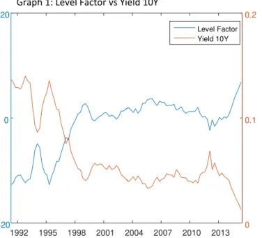
Figure 1.1: Ten Year Yield: Latent Factors, Fitted Values and Expectations Component
~
Notes: The top two panels of this figure plot the estimated level and slope factors of the affine term structure model against their empirical proxies: the 10Y Yield for the level factor and the Yield Spread for the slope factor. Graph 3 compares the model extracted expectations component of the 10Y Yield with the actual observed 10Y Yield and Graph 4 compares the actual observed 10Y Yields with the model fitted 10Y Yields.
1992 1995 1998 2001 2004 2007 2010 2013
-5 0 5
Graph 2:Slope Factor vs Yield Curve Slope
-0.05 0 0.05
Slope Factor Yield Slope (10Y-2Y)
1992 1995 1998 2001 2004 2007 2010 2013
-20 0 20
Graph 1: Level Factor vs Yield 10Y
0 0.1 0.2
Level Factor Yield 10Y
1992 1995 1998 2001 2004 2007 2010 2013 0
0.05 0.1 0.15
Graph 3: Observed 10Y Yield vs Expected 10Y Yield
Observed 10Y Yield Expected 10Y Yield
1992 1995 1998 2001 2004 2007 2010 2013 0
0.05 0.1 0.15
Graph 4: Yield curve Plot, Actual Yields vs Model Yields
Netherlands
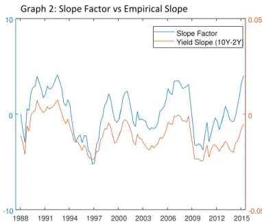
Figure 1.2: Ten Year Yield: Latent Factors, Fitted Values and Expectations Component
Notes: The top two panels of this figure plot the estimated level and slope factors of the affine term structure model against their empirical proxies: the 10Y Yield for the level factor and the Yield Spread for the slope factor. Graph 3 compares the model extracted expectations component of the 10Y Yield with the actual observed 10Y Yield and Graph 4 compares the actual observed 10Y Yields with the model fitted 10Y Yields.
1988 1991 1994 1997 2000 2003 2006 2009 2012 2015
-10 -5 0 5 10
15 Graph 1:Level Factor vs Yield 10Y
0 0.02 0.04 0.06 0.08 0.1
Level Factor Yield 10Y
1988 1991 1994 1997 2000 2003 2006 2009 2012 2015
-10 0 10
Graph 2: Slope Factor vs Empirical Slope
-0.05 0 0.05
Slope Factor Yield Slope (10Y-2Y)
1988 1991 1994 1997 2000 2003 2006 2009 2012 2015
-0.02 0 0.02 0.04 0.06 0.08 0.1
Graph 3: Observed 10Y Yield vs Expected 10Y Yield
Observed 10Y Yield Expected 10Y Yield
1988 1991 1994 1997 2000 2003 2006 2009 2012 2015
0 0.01 0.02 0.03 0.04 0.05 0.06 0.07 0.08 0.09 0.1
Graph 4: Yield curve Plot, Actual Yields vs Model Yields
Spain
Figure 1.3: Ten Year Yield: Latent Factors, Fitted Values and Expectations Component
Notes: The top two panels of this figure plot the estimated level and slope factors of the affine term structure model against their empirical proxies: the 10Y Yield for the level factor and the Yield Spread for the slope factor. Graph 3 compares the model extracted expectations component of the 10Y Yield with the actual observed 10Y Yield and Graph 4 compares the actual observed 10Y Yields with the model fitted 10Y Yields.
1992 1995 1998 2001 2004 2007 2010 2013
-20 -10 0 10
Graph 1:Level Factor vs Yield 10Y
0 0.05 0.1 0.15 Level Factor Yield 10Y
1992 1995 1998 2001 2004 2007 2010 2013
-7 -6 -5 -4 -3 -2 -1 0 1 2 3
Graph 2:Slope Factor vs Yield Curve Slope
-0.02 -0.01 -0.005 0 0.005 0.01 0.015 0.02 0.025 0.03 Slope Factor Yield Slope (10Y-2Y))
1992 1995 1998 2001 2004 2007 2010 2013
0 0.02 0.04 0.06 0.08 0.1 0.12
0.14 Graph 3: Observed 10Y Yield vs Expected 10Y Yield Observed 10Y Yield Expected 10Y Yield
1992 1995 1998 2001 2004 2007 2010 2013
0 0.02 0.04 0.06 0.08 0.1 0.12 0.14
Graph 4: Yield curve Plot, Actual Yields vs Model Yields
Germany
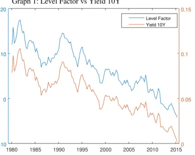
Figure 1.4: Ten Year Yield: Latent Factors, Fitted Values and Expectations Component
Notes: The top two panels of this figure plot the estimated level and slope factors of the affine term structure model against their empirical proxies: the 10Y Yield for the level factor and the Yield Spread for the slope factor. Graph 3 compares the model extracted expectations component of the 10Y Yield with the actual observed 10Y Yield and Graph 4 compares the actual observed 10Y Yields with the model fitted 10Y Yields.
1980 1985 1990 1995 2000 2005 2010 2015
-10 0 10 20
Graph 1:Level Factor vs Yield 10Y
0 0.05 0.1 0.15
Level Factor Yield 10Y
1980 1985 1990 1995 2000 2005 2010 2015
-10 0
10 Graph 2: Slope Factor vs Yield Curve Slope
-0.05 0 0.05
Slope Factor Yield Slope (10Y-2Y)
1980 1985 1990 1995 2000 2005 2010 2015
0 0.02 0.04 0.06 0.08 0.1 0.12
Graph 3: Observed 10Y Yield vs Expected 10Y Yield
Observed 10Y Yield Expected 10Y Yield
1980 1985 1990 1995 2000 2005 2010 2015
0 0.02 0.04 0.06 0.08 0.1 0.12
Graph 4: Yield curve Plot, Actual Yields vs Model Yields
Figure 2
: Developments in the 10Y Yield Term Premium
1992 1996 2000 2004 2008 2012
-0.02 -0.01 0 0.01 0.02 0.03 0.04 0.05 0.06 0,00 0,01 0,02 0,03 0,04 0,05
1980q1 1985q1 1990q1 1995q1 2000q1 2005q1 2010q1 2015q1
Graph 1: Term Premium 10Y Yield Germany
0 0,02 0,04 0,06 0,08
1993q1 1998q1 2003q1 2008q1 2013q1
Graph 2: Term Premium 10Y Yield Spain
Graph 3: Term Premium 10Y Yield Italy
0,000 0,005 0,010 0,015 0,020 0,025
1988q1 1993q1 1998q1 2003q1 2008q1 2013q1
Figure 3:
Probability of a Recession 2 quarters ahead from Alternative Probit Models
(
BBQ recessions are shown by the shaded regions)
0% 10% 20% 30% 40% 50% 60% 70% 80% 90% 100%
1991Q2 1996q2 2001q2 2006q2 2011q2
%
EH +TP Model Yield Curve Model
0% 10% 20% 30% 40% 50% 60% 70% 80% 90% 100%
1988q1 1993q1 1998q1 2003q1 2008q1 2013q1
%
Yield Curve Model EH +TP Model
0% 10% 20% 30% 40% 50% 60% 70% 80% 90% 100%
1991q1 1996q1 2001q1 2006q1 2011q1
%
Yield Curve Model EH +TP Model
0% 10% 20% 30% 40% 50% 60% 70% 80% 90% 100%
1991q3 1996q3 2001q3 2006q3 2011q3
%
Yield Curve Model EH +TP Model
Germany
Spain Italy
Table 4: Correlation Matrix State Variables vs Empirical Proxies
Table 3: Principal Component Analysis Bond Yields
Country Component Proportion Cummulative
Germany
Comp1 0,990 0,990
Comp2 0,009 0,999
Comp3 0,001 1,000
Italy
Comp1 0,995 0,995
Comp2 0.000 0.999
Comp3 0.000 1,000
Netherlands
Comp1 0,988 0,988
Comp2 0,010 0,999
Comp3 0,000 1,000
Spain
Comp1 0,992 0,992
Comp2 0,007 0,9994
Comp3 0,000 1,000
Country Empirical Proxies Level Factor Slope Factor
Germany Yield 10Y 99,95% 32,24%
Yield Slope -50,54% -96,57%
Italy Yield 10Y -98,97% -20,60%
Yield Slope 51,03% 89,08%
Netherlands Yield 10Y 99,80% 15,08%
Yield Slope -55,92% -92,34%
Spain Yield 10Y -98,41% -22,34%
Yield Slope 39,96% 93,43%
Table 5: LR Stability Test Statistics (1Q, 2Q, 3Q ahead)
Country test-statistic Break p-value break p-value break p-value
Germany Sup-LR 2008Q1 0,35 2007Q4 0,43 2007Q2 0,37
Exp-LR 2008Q1 0,43 2007Q4 0,60 2007Q2 0,33
Italy Sup-LR 2011Q2 0,00 2011Q1 0,00 2010Q4 0,00
Exp-LR 2011Q2 0,00 2011Q1 0,00 2010Q4 0,00
Netherlands Sup-LR 2011Q2 0,00 2011Q1 0,00 2010Q4 0,00 Exp-LR 2011Q2 0,00 2011Q1 0,00 2010Q4 0,00
Spain Sup-LR 2008Q2 0,00 2007Q4 0,00 2007Q3 0,00
Appendix A: Bry and Boschan Algorithm
The Bry and Boschan algorithm was created at the National Bureau of Economic Research
(NBER) as a tool for automatically capturing the phases of the Business cycle. It was designed to
replicate the decision-
making process of the NBER that defines “ a recession as a significant decline in
activity spread across the economy, lasting more than a few months, visible in industrial production,
employment, real income and trade”. A rec
ession begins just after the economy reaches a peak of
output and ends as the economy reaches its through. Between the through and the peak, the
economy is in an expansion.
The Bry- Boschan technique does not use any formal statistical framework to do the dating.
Instead it translates the NBER method into a simple set of decision rules. It basically comprises two
stages: (1) selecting the candidates for turning points and (2) applying a censoring rule to eliminate
the turns which do not satisfy some criteria. To the extent that the time frequency is quarterly we
adopt the methodology of Hardin and Pagan (2002) to locate the turning points of the cycle. The
automated dating algorithm BBQ is performed in Visual Basic under Excel, and can be summarized as
follows:
1. Identify a set of peaks and throughs by the application of a “turning point rule”. Let’s
𝑦
𝑡denote
the logarithm of real GDP at quarter t. So a local peak (resp. through) is reached at time t if and only
if
{𝑦
𝑡> 𝑦
𝑡+𝑘}
(resp.
{𝑦
𝑡< 𝑦
𝑡+𝑘})
for k=1,2.
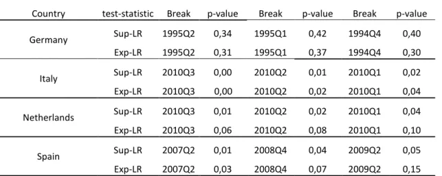
Table 5: LR Stability Test Statistics (4Q,5Q,6Q ahead)
Country test-statistic Break p-value Break p-value Break p-value
Germany Sup-LR 1995Q2 0,34 1995Q1 0,42 1994Q4 0,40
Exp-LR 1995Q2 0,31 1995Q1 0,37 1994Q4 0,30
Italy Sup-LR 2010Q3 0,00 2010Q2 0,01 2010Q1 0,02
Exp-LR 2010Q3 0,00 2010Q2 0,02 2010Q1 0,04
Netherlands Sup-LR 2010Q3 0,01 2010Q2 0,02 2010Q1 0,04 Exp-LR 2010Q3 0,06 2010Q2 0,08 2010Q1 0,10
Spain Sup-LR 2007Q2 0,01 2008Q4 0,04 2009Q2 0,05
2. Enforce the condition that peaks and throughs must alternate by selecting the highest (resp.
lowest) consecutive peaks (resp. throughs)
3. Turning points are censored according rules mainly relative to the duration of phases and cycles.
So an expansion or recession phase must be at least 2 quarters long. A complete cycle, defined by the
period of time between two peaks or throughs, must be at least 5 quarters in length. Complementary
rules are finally designed to avoid spurious turning points dating at the ends of the series.
The business cycles are thus obtained by the application of the BBQ algorithm to the real GDP series.
Table 2 in the appendix presents the estimate BBQ recession dates for the set of countries in our
dataset and summary statistics describing the cycle’s characteristics (duration and amplitude of the
phases).
Appendix B: Setup of the State Space system
The two factor affine term structure model described in the text is estimated using the Kalman filter
procedure. This can easily be done by transforming the model into its state space form:
The vector of observable data
𝑍
𝑡contains the bond yields for the 2,3,5,7 and 10 year maturities and
the matrices
𝐴
and
𝐻
, which link the state variables to the observed data are constructed by using
the
𝐴
𝑛~and
𝐵
𝑛~coefficients described in the text
𝑧
𝑡=
𝑍
𝑡[
𝑦
𝑡𝑖2 𝑦𝑒𝑎𝑟𝑦
𝑡𝑖3 𝑦𝑒𝑎𝑟𝑦
𝑡𝑖5 𝑦𝑒𝑎𝑟𝑦
𝑡𝑖7 𝑦𝑒𝑎𝑟𝑦
𝑡𝑖10 𝑦𝑒𝑎𝑟]
A =
[
𝐴
8~𝐴
12~𝐴
16~𝐴
20~𝐴
28~𝐴
40~]
H =
[
𝐵′
8~𝐵′
12~𝐵′
16~𝐵′
20~𝐵′
28~𝐵′
40~]
The coefficients
𝐴
𝑛and
𝐵
𝑛can be estimated recursively. The recursion begins with
𝐴
0= 0
e
𝐵
0= 0
.For
n=1,2,… the formulas are:
𝐵′
𝑛+1=
-
𝛿
1+
𝐵′
𝑛Ф ∗
;
𝐵′
~𝑛=
𝐵′𝑛𝑛𝑍
𝑡= 𝐴
+
𝐻𝑦
𝑡+ 𝑣
𝑡 (Measurement Equation)𝐴
𝑛+1=--
𝛿
0+ 𝐴
𝑛+ 𝐵
′𝑛µ*+
12𝐵
′𝑛𝐵
𝑛;
𝐴
𝑛~=
𝐴𝑛𝑛Ф ∗
=
Ф −
𝜆
1;
µ*= µ
1-
𝜆
0
The variance covariance matrix of the measurement errors
𝑣
𝑡is diagonal with diagonal elements
𝜎
12,
𝜎
2,2…
𝜎
52. The transition equation F is equal to the transition matrix
Ф(2𝑥2)
in the equation that
models the vector of the state factors as a vector autoregressive process of order 1:
𝐹 = Ф = [Ф(1,1) Ф(1,2)
Ф(2,1) Ф(2,2)]
The error term of the transition system is assumed to follow a multivariate normal distribution with
a variance covariance matrix equal to the identity matrix:
Q=
[
1 ⋯ 0
⋮ ⋱ ⋮
0 ⋯ 1
]
The initialization state vector and its variance covariance matrix are estimated using the stationarity
condition (state variables are covariance stationary). If {
𝑦
𝑡}
is covariance stationary, then each
𝑦
𝑡must
have constant mean and variance:
E(
𝑦
1/𝐹
0)
=
(𝐼
𝑚− Fy)
−1C
Vec(
𝑉
1) =
(𝐼
𝑚2− 𝐹⨂𝐹)
−1vec(Q),
with V1=Var(
𝑦
1/𝐹
0)
and where Vec(V1) is a column vector with dimensions
𝑚
2𝑥 1
and
⨂
is the
Kronecker tensor product.
Appendix C: Recursive Bond Prices
To derive the recursions in Eq. (7) we first note that for a one period bond, n=1, we have
𝑃
1𝑡
= 𝐸
𝑡[𝑀
𝑡+1] = 𝑒
−𝑟𝑡=
𝑒
−𝛿0−𝛿1𝑋𝑡Matching the coefficients leads to
𝐴
1= −𝛿
0and
𝐵′
1= −𝛿
1. Suppose that the price of an n- period
bond is given by
𝑃
𝑛𝑡=
𝑒
𝐴𝑛+𝐵′𝑛𝑋𝑡. Now we show that the exponential form also applies to the price of
the n+1 period bond:
𝑃
𝑛+1𝑡
=
𝐸
𝑡[𝑀
𝑡+1𝑝
𝑛𝑡+1]
=
𝐸
𝑡[𝑒𝑥𝑝 {−𝑟
𝑡−
12𝜒
′𝑡𝜒
𝑡− 𝜒
′𝑡𝜀
𝑡+1+ 𝐴
𝑛+ 𝐵′
𝑛𝑋
𝑡+1}]
=
=
𝑒𝑥𝑝 {−𝑟
𝑡−
12
𝜒
′𝑡𝜒
𝑡+ 𝐴
𝑛} 𝐸
𝑡[𝑒𝑥𝑝{−𝜒
′𝑡𝜀
𝑡+1+ 𝐵′
𝑛𝑋
𝑡+1}]
=
𝑒𝑥𝑝 {−𝑟
𝑡−
12
𝜒
′𝑡𝜒
𝑡+ 𝐴
𝑛} 𝐸
𝑡[𝑒𝑥𝑝{−𝜒
′𝑡𝜀
𝑡+1+ 𝐵
′𝑛(µ + Ф𝑋
𝑡+ ∑𝜀
𝑡+1}]
=
𝑒𝑥𝑝 {−𝛿
0+ 𝐴
𝑛+ 𝐵
′𝑛µ + (𝐵
′𝑛Ф − 𝛿
′1)𝑋
𝑡−
12
𝜆′
𝑡𝜆
𝑡}
x
𝐸
𝑡[𝑒𝑥𝑝{−(𝜒
′𝑡+ 𝐵
′𝑛∑)𝜀
𝑡+1}]
=
𝑒𝑥𝑝 {−𝛿
0+ 𝐴
𝑛+ 𝐵
′𝑛(µ − ∑𝜆
0) +
12