ISSN 0101-8205 www.scielo.br/cam
Step-size Estimation for Unconstrained
Optimization Methods
ZHEN-JUN SHI1,2 and JIE SHEN3
1College of Operations Research and Management, Qufu Normal University, Rizhao, Shandong 276826, P.R.China
2Institute of Computational Mathematics and Scientific/Engineering Computing, Academy of Mathematics and Systems Science, Chinese Academy of Sciences,
P.O. Box 2719, Beijing 100080, China 3Department of Computer & Information Science, University of Michigan, Dearborn, MI 48128, USA E-mails: [email protected] / [email protected] / [email protected]
Abstract. Some computable schemes for descent methods without line search are proposed. Convergence properties are presented. Numerical experiments concerning large scale uncon-strained minimization problems are reported.
Mathematical subject classification: 90C30, 65K05, 49M37.
Key words:unconstrained optimization, descent methods, step-size estimation, convergence.
1 Introduction
A well-known algorithm, for the unconstrained minimization of a function f(x)
innvariables
f: Rn→ R, (1)
having Lipschitz continuous first partial derivatives, is the steepest descent method (Fiacco, 1990, Polak, 1997, [8, 17]). The iterations correspond to the following equation
xk+1=xk−αk∇f(xk), k =0,1,2, ..., (2)
whereαk is the smallest nonnegative value ofαthat locally minimizes f along
the direction−∇f(xk)starting fromxk. Curry (Curry, 1944, [5]) showed that
any limit point x∗ of the sequence {x
k} generated by (2) is a stationary point
(∇f(x∗)=0).
The iterative scheme (2) is not practical because the step-size rule at each step involves an exact one-dimensional minimization problem. However, the steepest descent algorithm can be implemented by using inexact one-dimensional minimization. The first efficient inexact step-size rule was proposed by Armijo (Armijo, 1966, [1]). It can be shown that, under mild assumptions and with different step-size rules, the iterative scheme (2) converges to a local minimizer
x∗or a saddle point of f(x), but its convergence is only linear and sometimes slower than linear.
The steepest descent method is particularly useful when the dimension of the problem is very large. However, it may generate short zigzagging displacements in a neighborhood of a solution (Fiacco, 1990, [8]).
For simplicity, we denote∇f(xk)bygk, f(xk)by fkand f(x∗)by f∗,
respec-tively, wherex∗denotes a local minimizer of f. In the algorithmic framework
of steepest descent methods, Goldstein (Goldstein, 1962, 1965, 1967, [10, 11, 12]) investigated the iterative formula
xk+1=xk+αkdk, k =0,1,2, ..., (3)
wheredksatisfies the relation
gkTdk <0, (4)
which guarantees thatdk is a descent direction of f(x)atxk (Cohen, 1981,
No-cedal and Wright, 1999, [4], [14]). In order to guarantee the global convergence, it is usually required to satisfy the descent condition
gkTdk ≤ −ckgkk2, (5)
wherec>0 is a constant. The angle property
cosh−gk,dki = −
gkTdk
kgkk ∙ kdkk
is often used in many situations, withη0∈(0,1].
Observe that, ifkgkk 6=0 thendk = −gk satisfies (4), (5) and (6)
simultane-ously. Throughout this paper, we takedk = −gk.
There are many alternative line-search rules to chooseαk along the ray Sk =
{xk+αdk|α >0}. Namely:
(a) Minimization Rule. At each iteration,αk is selected so that
f(xk +αkdk)=min
α>0 f(xk+αdk). (7) (b) Approximate Minimization Rule. At each iteration,αkis selected so that
αk =min{α|g(xk+αdk)Tdk =0, α >0}. (8)
(c) Armijo Rule. Set scalarssk, γ ,L andσ withsk = − gT
kdk
Lkdkk2, γ ∈ (0,1), L>0 andσ ∈(0,12). Letαk be the largestαin{sk, γsk, γ2sk, ...,}such that
fk− f(xk+αdk)≥ −σ αgkTdk. (9)
(d) Limited Minimization Rule. Setsk = − gT
kdk
Lkdkk2 whereαk is defined by f(xk +αkdk)= min
α∈[0,sk]
f(xk+αdk), (10)
andL >0 is a given constant.
(e) Goldstein Rule. A fixed scalarσ ∈ (0,12)is selected, andαk is chosen in
order to satisfy
σ ≤ f(xk+αkdk)− fk
αkgTkdk
≤1−σ. (11)
(f) Strong Wolfe Rule. At thek-th iteration,αk satisfies simultaneously
fk− f(xk+αkdk)≥ −σ αkgkTdk (12)
and
|g(xk+αkdk)Tdk| ≤ −βgkTdk, (13)
(g) Wolfe Rule. At thek-th iteration,αksatisfies (12) and
g(xk+αkdk)Tdk ≥βgkTdk. (14)
Some important global convergence results for methods using the above men-tioned specific line search procedures have been given in the literature ([25, 15, 16, 23, 24]).
This paper is organized as follows. In the next section we describe some descent algorithms without line search. In Sections 3 and 4 we analyze their global convergence and convergence rate respectively. In Section 5 we give some numerical experiments and conclusions.
2 Descent Algorithm without Line Search
We assume that
(H1). f(x)is bounded below. We denoteL(x0)= {x ∈ Rn|f(x)≤ f(x0)}. (H2). The gradientg(x)is uniformly continuous on an open convex set B that
containsL0.
We sometimes further assume that the following condition holds.
(H3). The gradientg(x)is Lipschitz continuous on an open convex set B that contains the level setL(x0), i.e., there existsL such that
kg(x)−g(y)k ≤ Lkx−yk, ∀x,y∈ B. (15)
Obviously,(H3)implies(H2).
We shall implicitly assume that the constantLin (H3) is easy to estimate.
Algorithm (A).
Step 0. Choosex0∈ Rn,δ ∈(0,2)andL0>0 and setk :=0; Step 1. Ifkgkk =0 then stop; else go to Step 2;
Step 2. EstimateLk >0;
Step 3. xk+1=xk− Lδ
kgk;
Note. In the above algorithm, line search procedure is avoided at each iteration, which may reduce the cost of computation. However, we must estimate Lk at
each iteration. Certainly, if the Lipschitz constantLof the gradient of objective functions is known a priori, then we can takeLk ≡L in the algorithm. In many
practical problems, the Lipschitz constantL is not known a priori and we must estimate it and find an approximationLk toL at each step.
For estimatingLk we define
Lk =max
Lk−1,
kgk−gk−1k kxk−xk−1k
, k ≥1. (16)
We can also estimateLkin Algorithm (A) by solving the following
minimiza-tion problem
min
L∈R1kLδk−1−yk−1k, (17)
whereδk−1 = xk−xk−1,yk−1 = gk −gk−1andk ∙ kdenotes Euclidean norm. In this case,
Lk =max
Lk−1,
yT k−1δk−1 kδk−1k2
, k ≥1. (18)
Similarly,Lk can be found by solving the problem
min
L∈R1
yk−1−
1
Lk
δk
(19)
and set
Lk =max
Lk−1,
kyk−1k2
yT k−1δk−1
, k ≥1. (20)
The last two formulae are useful because they arise from the classical quasi-Newton condition (e.g. [14]) and from Barzilai and Borwein’s idea (1988, [2]). Some recent observations on Barzilai and Borwein’s method are very exciting (Fletcher, 2001, [7], Raydan 1993, 1997, [20, 21], Dai and Liao, 2002, [6]).
If the Hessian matrix∇2f(xk)is easy to evaluate then we can take
Lk =max{Lk−1,k∇2f(xk)k}, k ≥1. (21)
3 Convergence Analysis
Lemma 3.1 (mean value theorem). Suppose that the objective function f(x) is continuously differentiable on an open convex set B, then
f(xk+αdk)− fk =α
Z 1 0
dkTg(xk+tαdk)dt, (22)
where xk,xk +αdk ∈ B and dk ∈ Rn. Further, if f(x)is twice continuously
differentiable on B, then
g(xk+αdk)−gk =α
Z 1 0
∇2f(xk+tαdk)dkdt (23)
and
f(xk+αdk)− fk =αgkTdk+α2
Z 1 0
(1−t)dkT∇2f(xk+tαdk)dkdt. (24)
3.1 Convergence of Algorithm (A)
Theorem 3.1. If (H1) and (H3) hold, Algorithm (A) generates an infinite sequence{xk}, and
ρ∈
δ
2,1
, Lk ≥ρL,
+∞
X
k=0 1
L2
k
= +∞, (25)
then
lim inf
k→+∞ kgkk =0. (26)
Proof. By Lemma 3.1 and(H3)we have
f(xk+αdk)− fk = α
Z 1 0
dkTg(xk+tαdk)dt
= αgkTdk+α
Z 1 0
dkT(g(xk+tαdk)−gk)dt
≤ αgkTdk+α
Z 1 0
kdkk ∙ kg(xk+tαdk)−gkkdt
≤ αgkTdk+α2L
Z 1 0
tkdkk2dt
= αgkTdk+
1 2α
2Lkd
Takingdk = −gkandα= Lδ
k in the above formula, we have
f(xk−αgk)− fk ≤ −αkkgkk2+
1 2α
2
kLkgkk2
= −δkgkk 2
Lk
+ δ 2L 2L2
k
kgkk2
≤ −( δ Lk
− δ 2L 2L2
k
)kgkk2.
Noting thatLk ≥ρL, we obtain
δ Lk
−δ 2L 2L2
k
= 2δLk −δ 2L 2L2
k
≥ (2ρ−δ)δL 2L2k > 0.
Therefore,{fk}is a monotone decreasing sequence. So, by(H1),{fk}has a lower
bound and, thus,{fk}has a finite limit. It follows from the above inequality that
∞
X
k=0
(2ρ−δ)L
2L2k kgkk
2
<+∞. (27)
By (25) we have
∞
X
k=0
(2ρ−δ)L
2L2
k
= +∞.
The above inequality and (27) show that (26) holds. The proof is finished.
Corollary 3.1. If the conditions in Theorem 3.1 hold andρL ≤ Lk ≤ M
(M >0is a fixed large integer) for all k, then
∞
X
k=0
kgkk2<+∞, (28)
and, thus,
lim
Remark. The above theorem shows that we can set a largeLkto guarantee the
global convergence. However, ifLk is very large thenαk will be very small and
will slow the convergence rate of descent methods. On the other hand, very small values ofLk may fail to guarantee the global convergence. Thus, it is better to
set an adequate estimationLk at each iteration.
3.2 Comparing with other step-sizes
Theorem 3.2. Assume that the hypotheses of Theorem 3.1 hold. Denote the exact step-size byα∗
k (including exact line search rules (a) and (b)). Then
αk∗≥ ρ
δαk. (30)
Proof. For the line search rules (a) and (b), (H3)and Cauchy-Schwartz in-equality, we have:
αk∗Lkgkk2 ≥ kgk+1−gkk ∙ kgkk
≥ −(gk+1−gk)Tgk
= kgkk2.
Therefore,
α∗k ≥ 1
L.
Noting thatLk ≥ρL, we have
αk∗≥ 1
L ≥
ρ Lk
= δ
Lk
∙ρ
δ =αk∙ ρ
δ.
Theorem 3.3. Assume that the hypotheses of Theorem 3.1 hold. Denoteα∗
kthe
step-size defined by the line search rule (c) with L being the Lipschitz constant of∇ f(x). Then,
α∗k ≥ ρ
δαk, k ∈ K1; α ∗
k ≥
ργ (1−σ )
Proof. Ifk∈ K1, then
αk∗=sk =
1
L =
ρ ρL ≥
ρ δ ∙
δ Lk
= ρ
δαk.
Ifk∈ K2thenαk∗<skand thusα∗k/γ ≤sk, by line search rule (c), we have
f(xk+αk∗dk/γ )− fk > σ (αk∗/γ )g T kdk.
Using the Mean Value Theorem on the left-hand side of the above inequality, we see that there existsθk ∈ [0,1]such that
(αk∗/γ )g(xk+θkαk∗dk/γ )Tdk > σ (αk∗/γ )g T kdk,
and, thus,
g(xk+θkα∗kdk/γ )Tdk > σgkTdk. (32)
By(H3), Cauchy-Schwartz inequality and (32) we obtain:
αkLkdkk/γ ≥ kg(xk+θkα∗kdk/γ )−gkk ∙ kdkk
≥ [g(xk +θkαk∗dk/γ )−gk]Tdk
≥ −(1−σ )gkTdk.
Sincedk = −gk, by the above inequality, we get:
α∗k ≥ γ (1−σ )
L ≥
ργ (1−σ )
δ αk.
Theorem 3.4. Assume that the hypotheses of Theorem 3.1 hold. Denoteα∗kthe step-size defined by the line search rule (d) with L being the Lipschitz constant of∇ f(x). Then,
αk∗≥ ρ
δαk, (33)
whereαk is yet the step-size of Algorithm (A).
Proof. Ifαk∗=skthen
αk∗= 1
L =
ρ ρL ≥
ρ Lk
= ρ
Ifα∗
k <skthengkT+1dk =0 and, thus,
αk∗Lkdkk2≥ kgk+1−gkk ∙ kdkk ≥ −gkTdk.
Sincedk = −gk, by the above inequality, we get:
α∗k ≥ 1
L ≥
ρ ρL ≥
ρ Lk
= ρ
δαk.
Theorem 3.5. Assume that the hypotheses of Theorem 3.1 hold and letα∗
k be
defined by the line search rule (e). Then,
α∗k ≥ ρσ
δ ∙αk, (34)
Proof. By the line search rule (e), we have
f(xk+α∗kdk)− fk ≥(1−σ )αk∗g T kdk.
By the mean value theorem, there existsθksuch that
αk∗g(xk+θkα∗kdk)Tdk ≥(1−σ )αk∗g T kdk.
So,
g(xk+θkα∗kdk)Tdk ≥(1−σ )gkTdk. (35)
By(H3), the Cauchy-Schwartz inequality and (36), we have:
αk∗Lkdkk2 ≥ kg(xk+θkαk∗dk)−gkk ∙ kdkk
≥ [g(xk+θkα∗kdk)−gk]Tdk
≥ −σgkTdk.
Sincedk = −gk, we get:
αk∗≥ σ
L =
ρσ
ρL ≥ ρσ
Lk
= ρσ
δ αk.
Theorem 3.6. Assume that the hypotheses of Theorem 3.1 hold and thatαk∗is defined by the line search rules (f) or (g). Then,
αk∗≥ ρ(1−β)
Proof. By (13), (14) and the Cauchy-Schwartz inequality, we have:
α∗kLkdkk2 ≥ kgk+1−gkk ∙ kdkk
≥ [gk+1−gk]Tdk
≥ −(1−β)dkTdk.
Sincedk = −gkwe get:
α∗k ≥ 1−β
L =
ρ(1−β)
ρL ≥
ρ(1−β) Lk
= ρ(1−β))
δ αk.
4 Convergence Rate
In order to analyze the convergence rate of the algorithm, we make use of As-sumption(H4)below.
(H4). {xk} → x∗(k → ∞), f(x) is twice continuously differentiable on
N(x∗, ǫ)and∇2f(x∗)is positive definite.
Lemma 4.1. Assume that(H4)holds. Then,(H1), (H3)and thus(H2)hold
automatically for k sufficiently large, and there exists0<m′≤ M′andǫ
0≤ǫ
such that
m′kyk2≤ yT∇2f(x)y≤ M′kyk2, ∀x,y∈ N(x∗, ǫ0); (37) 1
2m
′
kx−x∗k2≤ f(x)− f(x∗)≤ 1 2M
′
kx−x∗k2, ∀x ∈ N(x∗, ǫ0); (38)
M′kx−yk2≥(g(x)−g(y))T(x−y)≥m′kx−yk2, ∀x,y ∈N(x∗, ǫ0); (39)
and thus
M′kx−x∗k2≥g(x)T(x−x∗)≥m′kx−x∗k2, ∀x ∈ N(x∗, ǫ0). (40)
By (39) and (40) we can also obtain, from Cauchy-Schwartz inequality, that
M′kx−x∗k ≥ kg(x)k ≥m′kx −x∗k, ∀x ∈ N(x∗, ǫ0), (41)
and
Lemma 4.2. If (H1) and(H3) hold and Algorithm (A) with Lk ≤ M and
L< M generates an infinite sequence{xk}, then there existsη >0such that
fk− fk+1≥ηkgkk2, ∀k. (43)
Proof. As in the proof of Theorem 3.1, we have:
fk− fk+1 ≥ (
δ Lk
− δ 2L 2L2k)kgkk
2
≥ (2ρ−δ)δL 2M2 kgkk
2
.
Taking
η= (2ρ−δ)δL 2M2 ,
we obtain the desired result.
Theorem 4.1. If the assumption(H4)holds, Algorithm (A) withρL ≤ Lk ≤ M
and L ≤ M generates an infinite sequence{xk}, then{xk}converges to x∗ at
least R-linearly.
Proof. By (H4), there existsk′such that xk ∈ N(x∗, ǫ0)fork ≥ k′. By (43) and Lemma 4.1 we obtain
fk− fk+1 ≥ ηkgkk2
≥ ηm′2kxk−x∗k2
≥ 2ηm ′2
M′ (fk− f ∗
), k ≥k′.
By (42) we can assume that M′ ≤ L and prove that θ < 1.In fact, by the
definition ofηin the proof of Lemma 4.2, we obtain
θ2 = 2m ′2η
M′ ≤
2m′2(2ρ−δ)δL
2M2M′ ≤
m′2(2σ−δ)δ
M′2 ≤(2ρ−δ)δ
m′2 M′2 ≤ (2ρ−δ)δ=2ρδ−δ2= −δ2−ρ2+2ρδ+ρ2=ρ2−(ρ−δ)2
Set
ω=p1−θ2.
Since, obviously,ω <1, we obtain from the above inequality that
fk+1− f∗ ≤ (1−θ2)(fk− f∗)
= ω2(fk− f∗)
≤ ...
≤ ω2(k−k′)(fk′+1− f∗).
By Lemma 4.1 and the above inequality we have:
kxk+1−x∗k2 ≤ 2
m′(fk+1− f ∗)
≤ ω2(k−k′)2(fk′+1− f ∗)
m′ .
Thus,
kxk−x∗k ≤ωk
r
2(fk′+1− f∗)
m′ω2(k′+1) .
This shows that{xk}converges tox∗at least R-linearly.
5 Numerical Experiments
We give an implementable version of this descent method.
Algorithm (A)′.
Step 0. Choosex0∈ Rn,δ ∈(0,2)andM ≫L0>0 and setk :=0; Step 1. Ifkgkk =0 then stop; else go to Step 2;
Step 2. EstimateLk ∈ [L0,M]; Step 3. xk+1=xk− Lδ
kgk;
Step 4. Setk :=k+1 and go to Step 1.
The following formulae forαk =δ/Lk(k ≥1):
1.
Lk =min
M,max
Lk−1,
yT k−1δk−1 kδk−1k2
2.
Lk =min
M,max
Lk−1,
kyk−1k2
ykT−1δk−1
(45)
3.
Lk =min
M,max
Lk−1, kyk−1k kδk−1k
(46)
4.
Lk =min
M,2(fk− fk−1+αk−1kgk−1k
2)
α2k−1kgk−1k2
(47)
are tried to compare the new algorithm against PR conjugate gradient method with restart and BB method ([2]). In conjugate gradient methods one has:
dk =
(
−gk, if k=0;
−gk+βkdk−1, if k ≥1,
(48)
where
βkF R = kgkk 2 kgk−1k2
, βkP R = g
T
k(gk−gk−1) kgk−1k2
, βkH S = g
T
k(gk−gk−1)
dkT−1gk−1
.
The corresponding methods are called FR (Fletcher-Revees), PR (Polak-Ribiére) and HS (Hestenes-Stiefel) conjugate gradient method respectively. Among them the PR method is regarded as the best one in practical computation. However, PR conjugate gradient method has no global convergence in many situations. Some modified PR conjugate gradient methods with global convergence were proposed (e.g., Grippo and Lucidi [9]; Shi [22], etc.). In PR conjugate gradient method, if gT
kdk ≥ 0 occurs, we set dk = −gk or setdk = −gk at every n
iteration. This is called restart conjugate gradient method (Powell [18]). We tested our algorithms with a termination criterion whenkgkk ≤epswith
method [2, 20, 21], which is sometimes superior to some CG methods [2]. The initial iterative points were also from the literature [13].
For PR conjugate gradient method with restart, we use Wolfe rule (g) with
β = 0.75, σ = 0.125. For our descent algorithms without line search, we choose the parametersδ =1, M =108and L
k defined by (44), (45), (46) and
(47) respectively. The corresponding algorithms are denoted by A1, A2, A3 and A4 respectively.
Failures in the application of the new method may appear, mainly due to the inadequate estimations ofLkand sometimes due to the roundoff errors. In order
to avoid failure, we check f(xk − Lδ
kgk) < fk in our numerical experiment. It
is obbserved thatδ ∈ (0,2) is an adjustable parameter in the gradient method without line search. We can adjustδto satisfy the descent property of objective functions and improve the performance of the new method. If f(xk−Lδ
kgk) < fk
holds then we continue the iteration. Otherwise, we may reduce δ by setting
δ=γ δwithγ ∈(0,1)until the descent property holds.
In numerical experiments, by Theorem 3.1, Lk may converge to+∞. Thus,
lettingLk ∈ [L0,M]seems to be unreasonable. In fact, we have no criteria to determineL0andM. Generally, a very large L0may lead to slow convergence rate and a very large M may violate the global convergence. As a result, we should choose carefully L0 and M in practical computation in order to satisfy both the global convergence and the fast convergence rate. Actually, we can combine the step-size estimation and line search procedure to produce efficient descent algorithms. For example, in Armijo’e line search rule, L > 0 is a constant at each iteration, and we can take the initial step-sizes = sk = 1/Lk
at the k-th iteration. In this case, the steepest descent method has the same numerical performance as our corresponding descent algorithm. Accordingly, choosing an adequate initial step-size is very important for Armijo’s line search and it is also the real aim of step-size estimation.
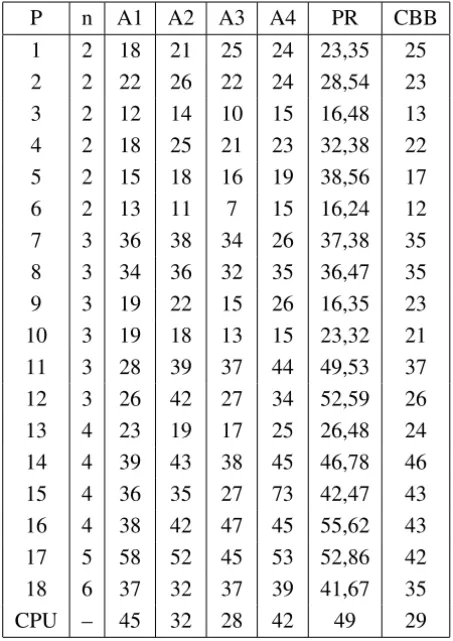
We use a Pentium IV portable computer and Visual C++ to implement our algorithms and test the 18 problems. The numerical results are reported in Table 1.
P n A1 A2 A3 A4 PR CBB
1 2 18 21 25 24 23,35 25
2 2 22 26 22 24 28,54 23
3 2 12 14 10 15 16,48 13
4 2 18 25 21 23 32,38 22
5 2 15 18 16 19 38,56 17
6 2 13 11 7 15 16,24 12
7 3 36 38 34 26 37,38 35
8 3 34 36 32 35 36,47 35
9 3 19 22 15 26 16,35 23
10 3 19 18 13 15 23,32 21
11 3 28 39 37 44 49,53 37
12 3 26 42 27 34 52,59 26
13 4 23 19 17 25 26,48 24
14 4 39 43 38 45 46,78 46
15 4 36 35 27 73 42,47 43
16 4 38 42 47 45 55,62 43
17 5 58 52 45 53 52,86 42
18 6 37 32 37 39 41,67 35
CPU – 45 32 28 42 49 29
Table 1 – Numerical results of algorithms onI N/F N(eps =10−8).
then less CPU time (seconds) than PR conjugate gradient with restart and CBB method in some situations. This also shows that CBB method is a promising method because it is superior to the new algorithms A1, A2 and A4 for these test problems.
The gradient method withLkdefined by (45) seems to be the best algorithm for
these test problems. Thereby, to estimateLk is the key to constructing gradient
methods without line search. If we take
αk =
1
Lk
= kδk−1k 2
δkT−1yk−1
or
αk =
δT k−1yk−1 kyk−1k2
,
whereδk−1 = xk −xk−1 and yk−1 = gk −gk−1, we can obtain Barzilai and
Borwein’s method ([2]) which is an effective method for solving large scale unconstrained minimization problems.
Conclusion
In future research we should seek more approaches for estimating the step-size as exactly as possible and find some available technique to guarantee both the global convergence and quick convergence rate of gradient methods. We can also use some step estimation approaches to improve the original BB method and conjugate gradient methods, for example, [19].
Acknowledgements. The work was supported in part by NSF DMI-0514900, Postdoctoral Fund of China and K.C.Wong Postdoctoral Fund of CAS grant 6765700. The authors would like to thank the anonymous referees and the editor for many suggestions and comments.
REFERENCES
[1] L. Armijo, Minimization of function having Lipschitz continuous first partial derivatives, Pacific J. Math.,16(1966), 1–13.
[2] J. Barzilai and J.M. Borwein, Two-point step size gradient methods, IMA J. Numer. Anal., 8(1988), 141–148.
[3] E.G. Birgin and J. M. Martinez, A spectral conjugate gradient method for unconstrained optimization, Appl. Math. Optim.,43(2001), 117–128.
[4] A. I. Cohen, Stepsize analysis for descent methods, J. Optim. Theory Appl.,33(2) (1981), 187–205.
[5] H. B. Curry, The method of steepest descent for non-linear minimization problems, Quart. Appl. Math.,2(1944), 258–261.
[6] Y. H. Dai and L. Z. Liao, R-linear convergence of the Barzilai and Borwein gradient method, IMA J. Numer. Anal.,22(2002), 1–10.
[8] A. V. Fiacco, G. P. McCormick, Nonlinear programming: Sequential Unconstrained Mini-mization Techniques, SIAM, Philadelphia, (1990).
[9] L. Grippo and S.Lucidi, A globally convergent version of the Polak-Ribiere conjugate gradient, Math. Prog.,78(1997), 375–391.
[10] A. A. Goldstein, Cauchy’s method of minimization, Numer. Math.4(1962), 146–150.
[11] A. A. Goldstein, On steepest descent, SIAM J. Control,3(1965), 147–151.
[12] A. A. Goldstein, J. F. Price, An effective algorithm for minimization, Numer. Math., 10(1967), 184–189.
[13] J. J. Moré, B. S. Garbow and K. E. Hillstrom, Testing unconstrained optimization software, ACM Trans. Math. Software,7(1981), 17–41.
[14] J. Nocedal and J. S. Wright, Numerical Optimization, Springer-Verlag New York, Inc. (1999).
[15] J. Nocedal, Theory of algorithms for unconstrained optimization, Acta Numerica,1(1992), 199–242.
[16] M. J. D. Powell, Direct search algorithms for optimization calculations, Acta Numerica, 7(1998), 287–336.
[17] E. Polak, Optimization: Algorithms and Consistent Approximations, Springer, New York, (1997).
[18] M. J. D. Powell, Restart procedure for the conjugate gradient method, Math. Prog., 12(1977), 241–254.
[19] M. Raydan and B. F. Svaiter, Relaxed steepest descent and Cauchy-Barzilai- Borwein method, Comput. Optim. Appl.,21(2002), 155–C167.
[20] M. Raydan, The Barzilai and Borwein method for the large scale unconstrained minimization problem, SIAM J. Optim.,7(1997), 26–33.
[21] M. Raydan, On the Barzilai Borwein gradient choice of steplength for the gradient method, IMA J. Numer. Anal.,13(1993), 321–326.
[22] Z. J. Shi, Restricted PR conjuate gradient method and its convergence(in Chinese), Advances in Mathematics,31(1) (2002), 47–55.
[23] P. Wolfe, Convergence condition for ascent methods II: some corrections, SIAM Rev., 13(1971), 185–188.
[24] P. Wolfe, Convergence condition for ascent methods, SIAM Rev.,11(1969), 226–235.
[25] Y. Yuan and W. Y. Sun, Optimization Theory and Methods, Science Press, Beijing (1997).