Copyright © 2005 SBMAC ISSN 0101-8205
www.scielo.br/cam
Matrix polynomials with partially
prescribed eigenstructure: eigenvalue sensitivity
and condition estimation
FERMIN S. VILOCHE BAZÁN*
Department of Mathematics, Federal University of Santa Catarina Florianópolis, Santa Catarina, 88040-900, Brazil
CERFACS Technical Report TR/PA/04/64 E-mail: [email protected]
Abstract. Let Pm(z)be a matrix polynomial of degreemwhose coefficients At ∈ Cq×q
satisfy a recurrence relation of the form: hkA0+hk+1A1+ ∙ ∙ ∙ +hk+m−1Am−1 = hk+m,
k≥0,wherehk= R ZkL ∈Cp×q, R∈Cp×n,Z =diag(z1, . . . ,zn)withzi 6=zjfori6= j,
0<|zj| ≤1, andL ∈Cn×q. The coefficients are not uniquely determined from the recurrence
relation but the polynomials are always guaranteed to havenfixed eigenpairs,{zj,lj},wherelj
is the jth column ofL∗. In this paper, we show that thezj’s are also theneigenvalues of an
n×nmatrixCA; based on this result the sensitivity of thezj’s is investigated and bounds for their condition numbers are provided. The main result is that thezj’s become relatively insensitive to
perturbations inCAprovided that the polynomial degree is large enough, the numbernis small,
and the eigenvalues are close to the unit circle but not extremely close to each other. Numerical results corresponding to a matrix polynomial arising from an application in system theory show that low sensitivity is possible even if the spectrum presents clustered eigenvalues.
Mathematical subject classification: 65F20,65F15.
Key words:matrix polynomials, block companion matrices, departure from normality, eigen-value sensitivity, controllability Gramians.
#616/04. Received: 09/IX/04. Accepted: 12/XII/04.
1 Introduction
We are concerned with matrix polynomials
Pm(z)= A0+z A1+ ∙ ∙ ∙ +zm−1Am−1−zmI, z ∈C, (1) whose coefficients At ∈ Cq×q (t = 0 :m−1)satisfy a recurrence relation of
the form
hkA0+hk+1A1+ ∙ ∙ ∙ +hk+m−1Am−1=hk+m, k =0,1,∙ ∙ ∙ (2)
where hk ∈ Cp×q. The coefficients, known as predictor parameters, reflect
intrinsic properties of the sequence{hk}such as frequencies, damping factors,
plane waves, etc, whose estimation from a finite data set{hk}Tk=0,is an important problem in science and engineering [1, 19, 20, 21, 22, 28]. In this work, we concentrate on polynomials arising in applications where the data are assumed to be modeled as
hk = R ZkL, k =0,1, . . . (3)
whereZ =diag(z1, . . . ,zn)withzi 6= zj fori 6= j, |zi| ≤1, R ∈ Cp×nis of
rank pandL ∈Cn×q of rankq with rows scaled to unit length. Also, as usual
in the applications of interest, we shall assume thatnis a small number.
Model (3) covers, e.g., impulse response samples of dynamic linear systems [1, 4, 19, 28, 29], where thez’s are system poles, time domain nuclear magnetic
resonance (NMR) data [26, 27], and time series defined by
hk = d X
j=1
fjcoskλj +gjsinkλj,
where fj,gj ∈Cp×1, thez’s are of the formzj =eıλj (ı = √
−1),n =2d,and
q =1 (see [22] and references therein).
In these applications, one wants to estimate the parameterszj and the matrices
where we assume thatm′ ≥m ≥ n, andn is the rank of the coefficient matrix,
then Pm(z)haszj(j =1:n)as eigenvalue andlj(j =1:n),the jth column
ofL∗, as associated left eigenvector [1, 19, 28] (the star symbol denotes
conju-gate transpose). Details about eigenvalues of matrix polynomials can be found in [12]. The remainingmq−neigenvalues have no physical meaning and are
commonly known asspurious eigenvalues. Once the eigenpairs{zj,lj}are
avail-able, the estimation ofRis straightforward. The same approach can be used in
the noisy data case but some criterion is needed to separate the eigenvalues of interest from the spurious ones.
Note that since{zj,lj}are eigenpairs of Pm(z),then there holds
l∗jPm(zj)=0, j=1:n. (4)
This is an underdetermined linear system of the form
KmXA =ZmL, (5)
where XT A =
AT
0 ∙ ∙ ∙ ATm−1
andKm is an n ×mq full-rank Krylov matrix
defined by
Km = [L Z L Z2L∙ ∙ ∙ Zm−1L]. (6)
Thus, all polynomials whose coefficients satisfy (2) (and hence (5)) will haven
fixed eigenpairs,{zj,lj}, but the remainder of their eigenstructure will depend on
the solution chosen. In the sequel we refer to thezj’s as prescribed eigenvalues
ofPm(z)and to the polynomial itself as a polynomial with partially prescribed
eigenstructure, or shortly, as a predictor matrix polynomial. For applications involving predictor polynomials, the reader is referred to [1, 19, 21, 25, 29, 22]. We observe also that associated with Pm(z)there is a block companion matrix
CAdefined by
CA=
0 0 ∙ ∙ ∙ 0 A0
Iq 0 ∙ ∙ ∙ 0 A1 0 Iq ∙ ∙ ∙ 0 A2
..
. ... . .. ... ...
0 0 ∙ ∙ ∙ Iq Am−1
. (7)
This matrix has the same eigenvalues as Pm(z)[12], left eigenvectors of the
formℓ∗= [l∗ zl∗∙ ∙ ∙zm−1l∗]withla left eigenvector of P
matrix equation
KmCA =ZKm. (8)
In practice the coefficients At are never known exactly and one has to
ana-lyze the sensitivity of thezj’s to perturbations in At.The problem has received
the attention of many researchers and many sensitivity analyses for the scalar case (i.e., for q = 1) are now available, see, e.g., [2, 6, 17, 21, 25]. Some
results concerning sensitivity of eigenvalues of general matrix polynomials can be found in [14, 24]. However, to the best of our knowledge nothing has been done on sensitivity analysis of prescribed eigenvalues of predictor polynomials forq > 1.The goal of this work is to carry out a sensitivity analysis of
pre-scribed eigenvalues only, focusing on the influence of the polynomial degree on such sensitivity. We show that this can be done by relating thezj’s to a small
n×nmatrix obtained by projectingCA onto an appropriate subspace and then
analyzing the projected eigenproblem. As a result, simple estimates of measures of sensitivity of thezj’s in the form of informative upper bounds are given.
The following notation is used throughout the paper. For A ∈ Cm×n, kAk2 and kAkF denote the 2-norm (or spectral) and Frobenius norm of A,
respec-tively. A† denotes the Moore-Penrose pseudo-inverse of A. The ith singular
value of Ais denoted byσi(A). The 2-norm condition number of A, κ(A), is
defined byκ(A)= kAk2kA†k2.The spectrum ofA∈Cn×nis denoted byλ(A). The identity matrix of ordernis denoted by Inand its jth column byej.
The paper is organized as follows. In Section 2, we describe results concern-ing the sconcern-ingular values of projected companion matrices by extendconcern-ing the work in [5]. The results obtained are then exploited in Section 3, in which we analyze the departure of the projected companion matrix from normality. In Section 4, we analyze the condition numbers of the zj’s introduced by Wilkinson [30],
sys-tems in diagonal form. Numerical results corresponding to a matrix polynomial arising from an application in system theory show that low sensitivity is possible even if some eigenvalues are clustered.
2 Singular value analysis of the projected companion matrix
In order to start our analysis we introduce a new block companion matrix asso-ciated with the prescribed eigenvalues. LetCBbe defined by
CB =
B0 Iq 0 ∙ ∙ ∙ 0
B1 0 Iq ∙ ∙ ∙ 0 ..
. ... . .. ... ...
Bm−2 0 ∙ ∙ ∙ 0 Iq
Bm−1 0 ∙ ∙ ∙ 0 0
(9)
whose first column block, denoted byXB,is any solution of the underdetermined
linear systemKmXB = Z−1L. This definition ensures thatz−j1(j =1:n) is an
eigenvalue ofCB and that there holds
KmCB = Z−1Km. (10)
Let the columns of V form an orthonormal basis for R(K∗
m),the column
space ofK∗
m. Notice that because of (8) and (10), R(Km∗) is a left invariant
subspace of bothCA andCB associated with the eigenvalues of interest. Let
CA(m,q)andCB(m,q)be the matrices obtained by projectingCAandCBonto
R(K∗
m),that is,
CA(m,q)=V∗CAV, CB(m,q)=V∗CBV. (11)
Then it is clear that
λ(CA(m,q))= {z1, . . .zn}, λ(CB(m,q))=
z−11, . . .z−n1 .
The goal of this section is to analyze the singular values ofCA(m,q), focusing
on their behavior as function ofm,q. Before proceeding we observe that when
understanding, these matrices will be denoted byCAandCB. Notice also that
the projector orthogonal ontoR(K∗
m), denoted byP, satisfies
P =V V∗=K†
mKm. (12)
Two lemmas are needed.
Lemma 2.1. For m ≥n and q≥1 there holds CA=C−B1.
Proof. SinceKmKm∗ is positive definite Hermitian, it is clear that the columns
ofV = K∗
m(KmK∗m)−1/2 form an orthonormal basis forR(Km∗). Using this
basis and the definitions ofCAandCBwe have
CACB=(KmKm∗)−1/2KmCAK∗m(KmK∗m)−1/2(KmKm∗)−1/2KmCBK∗m(KmK∗m)−1/2.
This reduces to identity on using (8), (10), and the fact thatKmKm† = I.
Lemma 2.2. Let A= A1A∗1−B1B1∗with A1∈Cn×pand B1∈Cn×q. Assume rank([A1 B1])= p+q <n.Then, the number of positive, negative, and zero
eigenvalues of A, is p, q, and n−(p+q), respectively.
Proof. Let the nonzero eigenvalues of A be arranged so that λ1(A) ≥ λ2(A) ≥ ∙ ∙ ∙ ≥ λp+q(A). Our proof relies on the minimax principle for
eigen-values [11]:
λk(A)= max
dim(S)=k x∈minS,x6=0
x∗Ax x∗x . Let the matrixP = [B1|A1]have a QR factorization
P =Q R = [Q1| Q2]
"
R11 R12 0 R22
#
, Q∗Q =Ip+q, (13)
where Q,R are partitioned such that Q1 ∈ Cn×q, Q2 ∈ Cn×p, R11 ∈ Cq×q,
R12 ∈ Cp×p and R22 ∈ Cp×p. Clearly, both R11 and R22 are nonsingular. From (13) it follows that
Substituting B1and A1into A, it follows that the projection of AontoR(Q2), the subspace spanned by the columns ofQ2, is
Q∗2A Q2= R22R∗22. (14) Let x ∈ R(Q2), x 6= 0. Then, because Q∗2A Q2 is positive definite by (14), puttingx =Q2β ∈Cp,β 6=0, we have
min
x∈R(Q2),x6=0
x∗Ax
x∗x ≥ x∈Rmin(Q2),x6=0
β∗Q∗2A Q2β
β∗β > 0,
and so, by the minimax principle, we conclude that A has at least p positive
eigenvalues. Considering matrix −A instead of A and proceeding as before
it follows that Ahas at leastq negative eigenvalues. Apart from this, it is clear
thatAhasn−(p+q)zero eigenvalues. From these conclusions the assertions
of the lemma follow.
In order to describe our results concerning the singular values of Cm,q, we
first notice that the Krylov matrix Km becomes a weighted Vandermonde
matrix whenq =1.When the weights are all ones this matrix will be denoted
byWm.Let the columns ofV˘ form an orthonormal basis forR(Wm∗). Then the
orthogonal projector ontoR(Wm∗),P˘, satisfies
˘
P =Wm†Wm = ˘VV˘∗. (15)
Using this notation we set
p1=Wm†e, x+=W
†
mZ m
e, (16)
where e= [1,∙ ∙ ∙ ,1]T ∈Rn.
We are now ready to describe the singular spectrum of matrixCA(m,q).
Theorem 2.3. Let the singular values of CA(m,q) be arranged so that σ1(CA) ≥ ∙ ∙ ∙ ≥ σn(CA). Assume that rank([ZmL L]) = 2q. Then, for
1≤q <n/2,there holds
σi(CA) >1 i=1:q,
σi(CA)=1, i=q +1:n−q,
0< σi(CA) <1 i=n−q+1:n.
Furthermore, if q = 1 the singular values of CA(m,1) do not depend on
the matrix L defined in (3), but rather on the Vandermonde matrix Wm. In
this case they are given by
σ12(CA(m,1)) = 1 2
2+ kx+k22− kp1k22+
q
kx+k22+ kp1k222−4|x0|2
σ2j(CA(m,1)) = 1, j =2:n−1.
σn2(CA(m,1)) = 1 2
2+ kx+k22− kp1k22−
q
kx+k22+ kp1k22
2
−4|x0|2
(18)
where x0denotes the first component of x+.
Proof. We use the fact that the squared singular values ofCA are eigenvalues
ofCAC∗A. In fact, using the definition ofCA,
CAC∗A=V∗CAV V∗C∗AV =V∗CAPC∗AV =V∗CAC∗AV. (19)
The last equality comes from the fact thatPC∗AV =C∗AVbecauseVis a basis of the right invariant subspace ofC∗Aassociated with prescribed eigenvalues. Now
notice that if we writeCA = [E2E2∙ ∙ ∙Em XA], where Ej denotes the block
column vector having its jth entry equal to Iqand the remaining ones equal to
the zero matrix, then
CAC∗A=E2E2∗+ ∙ ∙ ∙ +EmEm∗ +XAX∗A,
and this can be rewritten as
CAC∗A= Imq −E1E1∗+XAX∗A. (20)
Hence, using the fact that XA solves the system (5), which implies that
XA = X+A +N, where N is a matrix whose columns belong toN(Km) = [R(K∗
m)]⊥, we have
CAC∗A = In−V∗E1E1∗V +V∗X+AX+∗A V = In−V∗P1P1∗V +V∗X+AX+∗A V,
(21)
where
P1=K†mL =PE1, X+A =Km†Z mL
Now observe that [V∗X+
A V∗P1] = (V∗Km†)[Z mL L
] and that V∗K†
m is
nonsingular. From this and the assumption that rank([ZmL L
]) = 2q it
fol-lows that rank([V∗X+
A V∗P1])=2q. Thus, ifV∗X+A is identified with A1and
V∗P1with B1 in Lemma 2.2, it follows from (21) thatC
AC∗A hasn−2q zero
eigenvalues, the remaining ones being of the form 1+γi (i =1 :2q)withγi
the nonzero eigenvalues of−V∗P1P∗
1V +V∗X+AX+∗A V. Asq of theseγi are
positive and the otherq are negative, the inequalities in (17) follow, as desired.
To prove the statement of the theorem forq =1, we observe that in this case L is a column vector and that the Krylov matrix can be rewritten as Km =
L(1)W
m, whereL(1) =diag(L1,1, . . . ,Ln,1)is nonsingular since, by assumption
|Lj,1| =1, j=1:n. From this observation and pseudo-inverse properties, it is
immediate to see that P1reduces to p1, X+A reduces tox+, and neither depend
onL.Hence it follows thatCA(m,1)CA(m,1)∗does not depend onLand that
CA(m,1)CA∗(m,1)= In− ˘V∗p1p∗1V˘ + ˘V∗x+x+∗V˘.
The equalities (18) follow on analyzing the eigenvalues ofCA(m,1)C∗A(m,1)
from this equality; details can be found in [5].
Remark 1. The rank condition on[ZmL L]is no serious restriction in practice.
This is because in practical problemsL is dense, in which case one can prove,
under mild conditions, that rank([ZmL L])=2q.
Remark 2. Theorem 2.3 generalizes one concerning the singular values of a particular projected companion matrix by Bazan (see, Thm. 4 in [5]), and shows also that the singular values of the projected block companion matrix in our context, inherits to some extent the singular value properties of general block companion matrices described in Lemma 2.7 in [15].
Since the singular values ofCA(m,1)do not depend on the matrix L, we can
always compare the singular values ofCA(m,q)for the case whereq >1 with
Theorem 2.4. LetCA(m,q) as before. Then, for m ≥ n and 1 < q ≤ 2n,
there holds
σ1(CA(m,q))≤σ1(CA(m,1)), σn(CA(m,1))≤σn(CA(m,q)). (23)
Proof. We shall prove the inequalities (23) forq = 2; the proof for the case q >2 is similar. Notice that forq =1, we have
CA(m,1)C∗A(m,1)=In+ ˘V∗x+x+∗V˘ − ˘V∗p1p1∗V˘ =. In+E. (24)
while ifq =2,we have from (21)
CA(m,q)CA∗(m,q) =In+V∗X1X∗1V −V∗P11P11∗V
+ V∗X2X∗
2V −V∗P12P12∗V,
(25)
where we have assumed thatX+A = [X1,X2], P1 = [P11,P12].The idea behind the proof is to rewrite (25) in terms of the matrixE introduced in (24). For this we use the fact that
V∗X
i =TiV˘∗x+, V∗P1i =TiV˘∗p1, i =1,2. (26) whereTi =V∗IiV˘,I1 = [e1 e3 ∙ ∙ ∙ e2m−1], I2 = [e2 e4 ∙ ∙ ∙ e2m], in which
ei denotes theith canonical vector in Rmq. This can be seen as follows. Let
L= [L1,L2]andR1=diag(L1,1,∙ ∙ ∙ ,Ln,1). SinceZ andR1are diagonal, the
definition ofX1implies (see (22))
X1=Km†Z mL
1=K†mZ mR
1e=K†mR1WmWm†Z me
=Km†R1Wmx+. (27)
But since R1Wm =
R1e R1Z e ∙ ∙ ∙ R1Zm−1eandP=Km†Km, we have
Km†R1W =K†mL1Km†3L1 ∙ ∙ ∙ K†m3 m−1L
1= [Pe1Pe3 ∙ ∙ ∙ Pe2m−1]. Inserting this result in Eq. (27) yields
X1=Pe1Pe3 ∙ ∙ ∙ Pe2m−1x+. (28) A similar work withX2,P11, and P12gives
X2 = [Pe2Pe4 ∙ ∙ ∙ Pe2m]x+, (29)
P11 = Pe1Pe3 ∙ ∙ ∙ Pe2m−1p1, (30)
The set of equations (26) follows on multiplying byV∗on both sides of equations (28), (29), (30), and (31). Here we have used the fact that V˘V˘∗x+ = x+,
˘
VV˘∗p1= p1, since bothx+and p1belong toR(W∗
m).
We turn now to the proof of the theorem. Using the Eq. (26) and (24), we have
CA(m,q)C∗A(m,q)=In+T1ET1∗+T2ET2∗. (32) Letu be a unit vector in Cpand definew
i to be the unit vector with the same
direction asT∗
i u, i =1,2.Forming the Rayleigh-Ritz quotient in (32), we have
u∗CA(m,q)C∗
A(m,q)u = 1+w∗1Ew1kT1∗uk2+w2∗Ew2kT2∗uk2 ≤ 1+w∗Ew(kT∗
1uk2+ kT2∗uk2),
(33)
wherew =wi such thatw∗Ew=max{w∗1Ew1, w∗2Ew2}.Now using the
defi-nition of matrixT1, we have
kT∗
1uk2=u∗T1T1∗u=u∗V∗I1V˘V˘∗I1∗Vu = k ˘PI1∗Vuk2≤ kI1∗Vuk2, where we have used the fact thatP˘∗P˘ = ˘VV˘∗. A similar work gives
kT∗
2uk2 ≤ kI2∗Vuk2.
Summing up the two last inequalities it is not difficult to check that
kT∗
1uk2+ kT2∗uk2≤1. Substituting this result in (33) gives
u∗CA(m,q)C∗A(m,q)u≤w∗(I +E)w≤σmax2 (CA(m,1)),
and the proof of the first inequality in (23) is concluded.
Finally, since σn(CA(m,q)) = 1/σ1(CB(m,q)), by Lemma (2.1),
proceed-ing as before it followsσ1(CB(m,q)) ≤ σ1(CB(m,1)).This proves the second
inequality in (23) and the proof of the theorem is concluded.
A point that remains for discussion is the behavior of the singular values of CA(m,q) for fixed q ≥ 1 and varying m. This is a difficult problem; so we
Corollary 2.5 Let X+A and P1be as in(22). Then we have
q
1− kP1k22≤σn(CA), σ1(CA)≤ q
1+ kX+Ak22. (34)
Additionally, while the lower bound increases with m, the upper bound decreases.
Proof. First notice from (21) that the squared singular values ofCAthat differ
from 1 are the eigenvalues ofdefined by
= I2q+ "
X+∗A V −P1∗V
#
[V∗X+A V∗P1]
= "
Iq+X+∗A X+A X+∗A P1 −P1∗X+A Iq−P1∗P1
#
.
(35)
By comparing the eigenvalues ofwith those of its Hermitian part, it follows
λmin(Iq−P1∗P1)≤λi()≤λmax(Iq+X+∗A X+A).
This proves (34). We shall now prove that bothkX+Ak2andkP1k2are decreasing functions ofm. Let
˘
Km = [L Z L∙ ∙ ∙ZmL], X˘+A = ˘Km†Z
m+1L, k ˘P
1k2= ˘Km†L.
Then we shall prove thatk ˘X+Ak2 ≤ kX+Ak2andk ˘P1k2 ≤ kP1k2.In fact, write ˘
Km = [L |ZKm]and notice that
˘
Km†∗K˘†m =(K˘mK˘m∗)−1=(L L∗+ZGm,qZ∗)−1,
where
Gm,q =KmK∗m. (36)
Applying the Sherman-Morrison formula to the inverse above we obtain
˘
K†m∗K˘†m = Z−∗G−m1,qZ−1−Z−∗G−m1,qZ−1L(I+L∗Z−∗G−m1,qZ−1L)−1L∗Z−∗G−m1,qZ−1
= Z−∗Km†∗Km†Z−1−Z−∗Km†∗X+B(I+XB+∗X+B)−1X+∗B K
†
mZ−1,
(37)
where we have used the fact thatKmK†m = In, and we set X˘+B = ˘Km†Z−1L.
Pre-multiplication byL∗Zm+1∗and post-multiplication byZm+1Lon both sides of this equation yields
˘
This shows that the singular values of of X˘+A can not exceed those ofX+A, thus
ensuring the statement of the theorem for X+A. To prove thatkP1k2 decreases withm, it is sufficient to partitionK˘masK˘m = [Km | ZmL], and then proceed
as before.
The corollary is interesting because it provides a bound for the 2-norm condi-tion number ofCAof the form
κ(CA)≤ q
1+ kX+Ak22
q
1− kP1k22
(38)
that decreases withm.Thus, reliable bounds forκ(CA)can be obtained provided
both kX+Ak22 andkP1k22 are small enough. For the significant case where the prescribed eigenvalues lie inside the unit circle, the asymptotic of the bounds as
mis going to infinite is readily determined. To do this the following technical
result, the proof of which is straightforward, is needed.
Lemma 2.6. Suppose all zj fall inside the unit circle. ThenkX+Ak2 → 0as
m→ ∞.
Corollary 2.7. Suppose all zj lie inside the unit circle. Then, as m → ∞we
have
κ(CA)≤ n Y
j=1
|zj|−1.
Proof. We first notice that forq =1 we haveσ1(CA(m,1))σn(CA(m,1)) = Qn
j=1|zj|. Using Corollary 2.5 and Lemma 2.6 it follows that
lim
m→∞σ1(CA(m,q))=mlim→∞σ1(CA(m,1))=1.
Now sinceσn(CA(m,q)) ≥ σn(CA(m,1)) for allm ≥ n and fixedq > 1, by
Corollary 2.5 again, there holds
lim
m→∞σn(CA(m,q))≥mlim→∞σn(CA(m,1))= p Y
j=1
|zj|.
The assertion of the corollary follows on using this inequality and the definition
3 Departure from normality ofCA(m,q)
The influence of nonnormality on several problems in scientific computing has been known for long time and several measures of nonnormality either of theoretical or practical interest are now available [8, 10, 13]. An exhaus-tive discussion on the influence of nonnormality on many problems in scientific computing, using several measures of nonnormality, is given in Chaitin-Chatelin and Frayseé [8]. For A ∈ Cn×n the following measure has been introduced
by Henrici (1962):
D2(A) = kAk2F −
n X
j=1
|λj(A)|2. (39)
This measure plays an important role in our context because it can be related to the conditioning of the eigenbasis ofAwhen Ais diagonalizable. To clarify
this recall that for general A ∈ Cn×n with simple eigenvaluesλ
j anduj,vj as
associated left and right eigenvectors, the condition number ofλj, denoted by κj(λj), is defined by (see. e.g., Wilkinson [30, p. 314])
κ(λj)= k
ujk2kvjk2
|u∗jvj|
. (40)
Smith [23] proved that
κj(λj)≤ "
1+ 1
n−1
D
δj
2#(n−1)/2
, (41)
whereδj measures the distance ofλj to the rest of the spectrum. Thus the more
the ill-conditionedλj, the larger the ratioD/δj,which means that Dincreases
and/orδj is small. Another interpretation of the above result is possible. Of
course, it says that for the eigenvalueλj to be well conditioned, it suffices that
D/δj ≈0 andnbe a moderate number. We shall return to this point later.
The goal here is to analyze D(CA(m,q)),concentrating on its behavior as a
function ofm,qfor fixedq ≥1 and increasingm.The following theorem shows
that this can be made by comparing the singular values ofCA(m,q)with those
ofCA(m,1). This is always possible, since by Theorem 2.3, the singular values
Theorem 3.1. Let a and b denote respectively the largest and the smallest singular values ofCA(m,1)and let the singular valuesσjofCA(m,q)be ordered
in the usual way, i.e.,σ1≥σ2≥ ∙ ∙ ∙ ≥σn. Let
σ∗ = max
nσ1
a , σ2,∙ ∙ ∙, σn−1,
σn
b
o
, and
σ∗ = min
nσ1
a , σ2,∙ ∙ ∙ , σn−1,
σn b o . Define ˆ
k = σ
∗
σ∗, ρ=
a2−σ12
a2 (a
2
−1)+σ
2
n −b2
b2 (1−b
2). (42) Then, for eachm≥nand 1<q ≤n/2 it holds
kCA(m,1)k2F −ρ ≤ kCA(m,q)k2F
≤ q2(kˆ+ ˆk−1)2−(ρ+2q)+ kCA(m,1)k2F.
(43)
Proof. We first notice that, because of Theorem (2.3), we have
kCA(m,1)k2F =n−2+a
2
+b2. (44)
Now sinceCA(m,q)has the same spectrum asCA(m,1)we have
σ12σ22∙ ∙ ∙σq2σn2−q+1∙ ∙ ∙σn2−1σn2= n Y
j=1
|zj|2=a2b2. (45)
If this is rewritten as
1= a2
σ12
1
σ22∙ ∙ ∙
1
σq2
1
σn2−q+1
1
σn2−q+2∙ ∙ ∙
1
σn2−1
b2
σn2,
the geometric-arithmetic mean inequality leads to
2q ≤ a
2
σ12 +
1
σ22 + ∙ ∙ ∙ +
1
σp2 +
1
σn2−p+1 + ∙ ∙ ∙ +
1
σn2−1 +
b2
σn2.
Multiplying both sides of this inequality by the sum of the reciprocals of each term of the right hand side, we obtain
σ12
a2 +σ
2
2 + ∙ ∙ ∙ +σq2+σ
2
n−p+1+ ∙ ∙ ∙ +σn2−1+
σn2
b2
where
A = diag(σ12/a2, σ22, . . . , σq2, σn2−q+1, . . . , σn2−1, σn2/b2),
c = [1,1, . . . ,1]T ∈R2q.
Kantorovic’s inequality (see Horn and Johnson [16, Thm. 7.4.41]) leads then to
σ2 1
a2 +σ
2
2 + ∙ ∙ ∙ +σq2+σ
2
n−p+1+ ∙ ∙ ∙ +σn2−1+
σn2
b2
2q ≤
h
q(kˆ+ ˆk−1)
i2
,
wherekˆis defined in (42). Hence it follows
σ12+ ∙ ∙ ∙ +σn2≤ q
2(kˆ+ ˆk− 1)2
+σ12−σ
2 1
a2 +σ
2
n − σn2
b2 +n−2q. (46)
The upper bound in (43) follows from this inequality on noting that
σ12− σ
2 1
a2 +σ
2
n − σn2
b2 = −ρ+a
2
+b2−2, (47)
whereρis defined in (42). To prove the lower bound, rewrite (45) as
1 = σ12
a1
σ22∙ ∙ ∙σq2σn2−q+1σn2−q+2∙ ∙ ∙σn2−1σ
2
n
b2.
The geometric-arithmetic mean inequality leads then to
2q ≤ σ
2 1
a12 +σ
2
2 + ∙ ∙ ∙ +σq2+σn2−q+1+σn2−q+2+ ∙ ∙ ∙ +σn2−1+
σn2
b2
The lower bound in (43) is a consequence of using (47) in this inequality.
The departure from normality of CA(m,1) is analyzed in Bazan [5]. The
conclusion drawn from that analysis is that this matrix becomes close to a normal matrix provided the eigenvalues zj fall near the unit circle and m is
large enough. This is important in our context since if we take into account the inequalities (43), we can conclude thatCA(m,q)for the caseq >1 may
be-come closer to normality thanCA(m,1).In terms of eigenvalue sensitivity, this
means that prescribed eigenvalues ofPm(z)can be less sensitive to noise when
regarded as eigenvalues ofCA(m,q)withq >1 than when regarded as
eigen-values ofCA(m,1).This shall be theoretically demonstrated in the next section.
Example: departure from normality ofCA(m,q)arising from a dynamical
system. The dynamical system under analysis is defined by the state space equations
˙
x = Ax+Bu
y =C x, (48)
and corresponds to a computer model of a flexible structure known as Mini-Mast [18]. Matrices A,B and C are of orders 10×10, 10×2 and 2×10,
respectively; the entries of the matrices can be found in [18]. Impulse response samples are thus given as
hk =CeA1tkB, k =0,1, . . .
MatricesRandLof model (3) are thus of order 2×10 and 10×2, respectively,
and can be found readily by computing an eigendecomposition of matrix A.
According to our notation this implies thatn =10,p =q =2;the eigenvalues
are of the formzj =esj1t (j =1:10)where thesj’s are eigenvalues of A. The
time step is1t=0.03s. The model comprises five modes (in complex conjugate
pairs) and involves two closely spaced frequency pairs. Frequencies and damping expressed as the negative real part of thezj’s as well as the eigenvalues in modulus
and separationsδj =min|zj −zi|, i6= j,are displayed in Table 1.
Mode Damping Frequency |zj| δj
j rad/s
1 0.32907 27.42011 0.99017 0.32299 2 0.38683 38.68230 0.98846 0.00982 3 0.38352 38.35103 0.98856 0.00982 4 0.09066 5.03555 0.99728 0.00011 5 0.09055 5.03176 0.99728 0.00011
Table 1 – System poleszj and separations.
In order to illustrate the behavior of D2(CA(m,q))as a function ofm,q the
normskCA(m,q)k2F for increasingm andq = 1:2 were computed from the
relation (see (21))
10 20 30 40 50 60 70 80 90 100 -8
-6 -4 -2 0 2 4 6 8 10 12
q = 1
q = 2
m
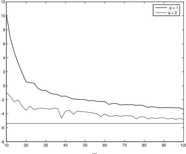
Figure 1 – Departure from normality of matrixCA(m,q)as a function ofmandq on a logarithmic scale; q denotes the number of columns of matrix L in (3) andm the degree ofPm(z).The horizontal line points out the asymptotic value ofD2(CA(m,2)) for largem.
All computations were carried out using MATLAB. The results displayed in Figure 1 are surprising: they not only show thatD2(CA(m,2))really improves
D2(CA(m,1))but also that this improvement can be dramatic whenm is near
n=10. For illustration, while forq =1 andm =10,11 we obtain
D2(CA(10,1))=2.5877×10⁴, D2(CA(11,1))=3.692×10³,
which illustrate thatCA(10,1)andCA(11,1)are highly nonnormal, forq =2
and the same values ofmwe obtain
D2(CA(10,2))=5.4295×10⁻¹, D2(CA(11,2))=4.9053×10⁻¹
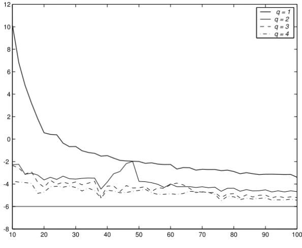
The influence ofq on D2(CA(m,q))forq > 2 was also analyzed. For this,
10 20 30 40 50 60 70 80 90 100 -8
-6 -4 -2 0 2 4 6 8 10 12
q = 1 q = 2 q = 3 q = 4
m
Figure 2 – Departure from normality of matrixCA(m,q)as a function ofmandq on a logarithmic scale; q denotes the number of columns of matrix L in (3) andm the degree ofPm(z).The horizontal line points out the asymptotic value ofD2(CA(m,4)) for largem.
were constructed. With these matrices at hand, the matrices L of
correspond-ing orders were obtained in the same way as in the case for q = 2.Results
corresponding to the seed value of the random generator equal to 10 (we use the MATLAB functionrandn), displayed in Figure 2, show once more that the
departure from normality of matrixCA(m,q)forq > 1 gets smaller than that
corresponding toq =1.However no conclusion can be drawn concerning the
be-havior ofD2(CA(m,q))for valuesq >2 in comparison with that corresponding
toq =2.
As in this example all eigenvalues lie inside the unit circle, the asymptotic value of D2(CA(m,q)) as m is going to infinity can be readily computed: it
suffices to use (49) taking into account that in this case
where
G∞,q= lim
m→∞Gm,q =mlim→∞KmK
∗
m, with [Gm,q]i,j =e∗iL L∗ej
1−(zizˉj)m
1−ziˉzj .
Asymptotic values ofD2(CA(m,q))in this case are:
D2(CA(∞,1))=0.9719×10⁻², D2(CA(∞,2))=0.4915×10⁻²,
D2(CA(∞,3))=0.2946×10⁻², D2(CA(∞,4))=0.2489×10⁻²
4 Condition numbers
We have seen that the prescribed eigenvalueszj of Pm(z)are eigenvalues of the
projected companion matrixCA(m,q).This fact is exploited here to carry out a
sensitivity analysis of these eigenvalues. To this end , we choose as measures of sensitivity the Wilkinson condition numbers of the zj’s (see (40)) viewed
as eigenvalues of CA(m,q),and the overall 2-norm condition number of the
eigenvalue problem. In order to describe our results we recall that form ≥ n
and fixedq,q ≥1,Gm,q =KmK∗mis positive definite Hermitian. In the sequel
we shall always assume that the left eigenvector ofPm(z)(the rows of matrixL
in (3)) are scaled using the 2-norm to unit length. The lemma below explains that the sensitivity of the eigenvalue problem associated with matrixCA(m,q)
is governed by the condition number of matrixGm,q.
Lemma 4.1. LetCA(m,q)be as before. Then there holds
CA(m,q)=(Gm,q)−1/2Z(Gm,q)1/2.
Consequently, the sensitivity of the eigenvalue problem related to the prescribed eigenvalues is governed bypκ(Gm,q).
Proof. SetV =K∗
m(Gm,q)−1/2. It is immediate to check that the columns of
V form an orthonormal basis ofR(K∗
m).Using the definition ofCA(m,q)and
this basis, we have
CA(m,q) = V∗CAV
= (Gm,q)−1/2KmCAK∗m(Gm,q)−1/2.
In the following, the condition number of zj related to CA(m,q) forq > 1
(and hence to Pm(z)) is denoted byκq(zj), while the condition number of the
same eigenvalue but related toCA(m,1)is denoted byκ1(zj).
Theorem 4.2. For m≥n the following properties hold
(a) For1≤q ≤n/2we have
κq(zj)= q
1+ |zj|2+ |zj|4+ ∙ ∙ ∙ + |zj|2(m−1)kKm†ejk2 (j =1:n). (50) (b) The condition numbersκ1(zj)do not depend on the matrix L but rather
on the Vandermonde matrix Wm.
(c) For fixed m≥n and q>1there holdsκq(zj)≤κ1(zj).
(d) Letδj = min 1≤k≤n 1≤j≤n,j6=k
|zj −zk|Then, for1≤q ≤n/2there holds
κq(zj)≤ "
1+ n−1+ kx +k2
2+Qnj=1|zj|2−Pnj=1|zj|2 (n−1)δ2j
#(n−1)/2
, (51)
where x+ denotes the minimum norm solution of the system(5) for the case q =1.
Proof. To prove(a)notice from Lemma 4.1 thatvj =Gm−,1q/2ejanduj =Gm1/,2qej
are left and right eigenvectors of CA(m,q), respectively, associated with the
eigenvaluezj. These eigenvectors satisfy the conditionu∗jvj =1.Besides this
kvjk22=v∗jvj =e∗jGm−1,qej = kKm†ejk22,
and
kujk22 =e∗jGm,qej = kK∗mejk22=1+ |zj|2+ |zj|4+ ∙ ∙ ∙ + |zj|2(m−1).
The last equality is because the rows of L in (3) are scaled to unit length by
assumption. The equality (50) follows from these relations on using the defini-tions given in (40).
To prove property(b)notice thatLbecomes a column vector inCnwhenq =1.
matrix with the components of L as entries andWm the Vandermonde matrix
introduced in the previous section. From this observation and the definition (40) it is immediate that
κ1(zj)= ke∗jWmk2kWm†ejk2,
which proves(b).
The proof of (c)is based on the property that kK†mejk2 ≤ kWm†ejk2, which can be seen as follows. Letφj = K†mej.This means thatφj is the minimum
2-norm solution of the underdetermined linear system
Kmφ =ej. (52)
LetKem = [L(1)Wm∙ ∙ ∙L(q)Wm],where L(i) =diag(L1,i, . . .Ln,i),i =1. . .q.
It is clear thatK˜m =KmJwithJan appropriate permutation matrix. Introduce ˜
KD
m defined by
˜ KD
m =
Wm†L(1)
.. .
Wm†L(q) .
Then
˜
KmK˜mD =L
(1)L(1)∗+ ∙ ∙ ∙L(q)L(q)∗=I
n,
and thereforeK˜D
m is a right inverse of Kem.Define nowφ = JK˜mDej.It is not
difficult to check that this vector is a solution of the system (52). Additionally
kφk22 = kWmejk22|Lj,1|2+ kWmejk22|Lj,2|2+ ∙ ∙ ∙ + kWmejk22|Lj,q|2 = kWmejk22(|Lj,1|2+ |Lj,2|2+ ∙ ∙ ∙ + |Lj,q|2)
= kWmejk22.
This equality proves property (c) asφj is the solution of minimum norm of (52).
Finally, property (d) is a consequence of estimate (41), property (c), and
Lemma 7 in Bazán [5] where it is proved that
D2(CA(m,1))≤n−1+ kx+k22+ n Y
j=1
|zj|2− n X
j=1
|zj|2.
depends on intrinsic characteristics of the eigenvalues themselves and on the degree of the associated matrix polynomial. Concerning the estimates (51), since
nis assumed to be small, the conclusion is that they can approach the optimum
value 1 providedkx+k22≈0 and the eigenvalues in modulus are reasonably close
to the unit circle but not extremely close to each other. In spite of the fact that this conclusion seems to emerge under rather stringent conditions, namely,n small
andzj’s close to the unit circle, we emphasize that there are many applications in
which these conditions appear frequently. In fact, in modal analysis of vibrating structures, the analysis of slow-decaying signals often involves eigenvalues very close to the unit circle andn small; in [4, 1, 19] examples are reported with n ranging from 15 to 20. Numerical examples showing thatkx+k22 ≈ 0 for
moderate values of m are discussed in [7]. Another example involving the
condition n small is encountered in NMR; genuine applications in this field
point outnranging from 2 to 16 [26, 27]. The conditionkx+k22≈0 in NMR is
numerically verified in [3].
Apart from the conclusion above, a remark concerning the meaning of prop-erty(c)must be done: It predicts reduction in sensitivity of prescribed
eigenval-ues when extracted from projected companion matrices related to polynomials withq >1.This will be illustrated numerically later.
The following theorem states that the conditioning of the eigenvalue problem associated withCA(m,q)improves the conditioning of the eigenvalue problem
associated with matrixCA(m,1).
Theorem 4.3. SetG˘m =WmWm∗. Then for each m≥n, we have that
κ(Gm,q)≤κ(G˘m).
Proof. We shall prove that
λ1(Gm,q)≤λ1(G˘m), and λn(Gm,q)≥λn(G˘m). (53)
In fact, letKem be as in the proof of the previous theorem. Then it is clear that ˜
KmK˜m∗ =Gm,q. Using this result, for all unit vectoru ∈Cn, we have that
u∗Gm
,qu = u∗K˜mK˜m∗u = u∗L(1)G˘
Letvj (j =1:q)be the unit vector with the same direction asL(j)∗u.
Substi-tutingvj in the above equation and using the Rayleigh-Ritz characterization of
eigenvalues of symmetric matrices, we get
u∗Gm,qu = v1∗G˘mv1kL(j)∗uk2+ ∙ ∙ ∙ +vq∗G˘mvqkL(q)∗uk2 ≤ λ1(G˘m)(kL(j)∗uk2∙ ∙ ∙ + kL(q)∗uk2).
The first inequality in (53) follows on noting that(kL(j)∗uk2∙ ∙ ∙+kL(q)∗uk2)=1 because by assumption all rows of L have 2-norm equal to one. The second
inequality in (53) follows in the same way and the proof concludes.
Note that because of its definition, whenever allzj fall inside the unit circle,
the limit ofGm,q asm → ∞is always guaranteed to exist, and the same result
applies forG˘m.
Corollary 4.4. LetG∞,qdenote the limiting value ofGm,qas m→ ∞. Suppose
all prescribed eigenvalues zj of Pm(z)fall inside the unit circle. Define
α =max|zj|, β =min|zj|, and δ=min|zi−zj|, i6= j, 1≤i, j≤n.
Then
κ(G∞,q) ≤
1 2
η+pη2−4,
where
η=n
"
1+ n−1+
Qn
j=1|zj|2−Pnj=1|zj|2 (n−1)δ2
#(n−1)/2 s 1−β2
1−α2 −n+2
Proof. This corollary is a consequence of Theorem 4.3 and Corollary 9 in
Bazán [5].
Example: conditioning of Mini-Mast eigenvalues. To confirm the theore-tical predictions of Theorem 4.2 we have computed the condition numbersκq(zj)
of the eigenvalues associated with the Mini-Mast model described in the previous section. The goal is to verify that severe reduction in sensitivity is possible when extracting thezj’s from projected companion matrices related to polynomials
Mode κ1(zj) κ1(zj) κ2(zj) κ2(zj) κ3(zj) κ4(zj)
j m=10 m=20 m=10 m=20 m=10 m=10
1 0.00017×10⁷ 0.00130×10³ 1.77339 1.00929 1.19281 1.12292 2 0.00127×10⁷ 0.02310×10³ 2.30402 1.50635 1.19617 1.04022 3 0.00136×10⁷ 0.02311×10³ 1.64077 1.49986 1.13957 1.08176 4 3.10889×10⁷ 4.75131×10³ 7.56466 3.86546 1.75153 1.19145 5 3.11084×10⁷ 4.75306×10³ 8.07200 3.86827 1.37293 1.29589
Table 2 – Condition numbers of prescribed eigenvalueszj.
4.1 An application to linear system theory
We shall show that the Corollary 4.4 can be applied to estimating the 2-norm condition number of controllable Gramians in linear system theory. Consider a dynamical discrete linear systemSdescribed by the state equations
xk+1 = Axk+Buk
yk = C xk
(54)
whereA∈Rn×n,B∈Rn×q, andC∈Rq×n. Assumeλi(A)6=λj(A), fori 6= j,
and|λi(A)|<1 (i =1 :n). Assume also that the system is controllable, i.e.,
the extended controllable matrixCmq defined by
Cq
m = [B A B A
2B
∙ ∙ ∙Am−1B], m ≥n,q ≥1 (55)
satisfies rank(Cmq)=n.Then the controllable Gramian of the systemS, defined
as [9]
Q=
∞ X
j=0
B AjAj∗B∗, (56)
is guaranteed to be symmetric and positive definite, and its eigenvalues are known to concentrate information that plays a crucial role when solving sys-tem identification and model order reduction problems. It turns out that if the system eigenvalues λj(A) are distinct, a change of basis of the state vector bxk =T−1xkwithT a matrix of right eigenvectors ofA, will transform the state
space representation (54) to another one in diagonal form. When this is done, Cmq reduces to a matrix like the block Krylov matrixKm and the controllable
GramianQreduces to one likeG∞,q.This shows that the estimate forκ(G∞,q)
5 Conclusions
Based on the fact that prescribed eigenvalues of predictor polynomials can be regarded as eigenvalues of projected block companion matrices, an eigenvalue sensitivity analysis was performed. As a result, simple estimates of measures of eigenvalue sensitivity in the form of informative upper bounds were derived. In particular, under the assumption thatnis small, it was proved that prescribed
eigenvalues near the unit circle can be relatively insensitive to noise provided the polynomial degree is large enough. The effect of the dimension of the coeffi-cients on the sensitivity was also analyzed and it was concluded that prescribed eigenvalues of predictor polynomials can be less sensitive to noise when regarded as eigenvalues of projected companion matrices related to matrix polynomials with coefficients of orderq >1 than when regarded as eigenvalues of projected
companion matrices related to scalar polynomials. The theory was numerically illustrated using a matrix polynomial with clustered eigenvalues arising from the modal analysis field. The results are of interest in system analysis where estimates for the 2-norm condition number of controllability Gramians of multi-input multi-output discrete dynamical systems play a crucial role.
The author is aware that further research is desirable for the case where the pre-scribed eigenvalues are almost defective: the bounds in property (d) of Thm. 4.2 can be pessimistic in this case as the ratio D/δj is no longer small, but as
il-lustrated in Table 2, the conditioning itself remains excellent. Furthermore, an analysis for the case where the prescribed eigenvalues are defective is needed. This challenging development is the subject of future research.
Acknowledgments. The author wishes to thank I.S. Duff and members of the ALGO Team at CERFACS for providing a cordial environment. Special thanks go to S. Gratton for suggestions that have improved the presentation of the paper. Thanks also go to the referees for their suggestions and constructive criticism. The author is particularly grateful to one referee for an important observation concerning inequality (51).
REFERENCES
[2] F.S.V. Bazán, Error analysis of signal zeros: a projected companion matrix approach, Linear Algebra Appl.,369(2003), 153–167.
[3] F.S.V. Bazán, CGLS-GCV: a hybrid algorithm for solving low-rank-deficient problems. Appl. Num. Math.,47(2003), 91–108.
[4] F.S.V. Bazán and C.A. Bavastri, An optimized Pseudo inverse algorithm (OPIA) for multi-input multi-output modal parameter identification, Mechanical Systems and Signal Process-ing,10(1996), 365–380.
[5] F.S.V. Bazán, Conditioning of Rectangular Vandermonde Matrices with nodes in the Unit Disk, SIAM J. Matrix Analysis and Applications,21(2) (2000), 679–693.
[6] F.S.V. Bazán and Ph.L. Toint, Error analysis of signal zeros from a related companion matrix eigenvalue problem, Applied Mathematics Letters,14(2001), 859–866.
[7] F.S.V. Bazán and Ph.L. Toint, Singular value analysis of predictor matrices, Mechanical Systems and Signal Processing,15(4) (2001), 667–683.
[8] F. Chaitin-Chatelin and V. Frayssé, Lectures on Finite Precision Computations. SIAM, Philadelphia (1996).
[9] Chi-T. Chen, Linear System theory and Design, Third Edition, Oxford University Press, New York (1999).
[10] L. Elsner and M.C. Paardekooper, On measures of nonnormality of matrices, Linear Algebra Appl.,92(1987), 107–124.
[11] G.H. Golub and C.F. Van Loan, Matrix Computations, The Johns Hopkins University Press, Baltimore (1996).
[12] I. Gohberg, P. Lancaster and L. Rodman, Matrix Polynomials, Academic Press, New York (1982).
[13] P. Henrici, Bounds for iterates, inverses, spectral variation and field of values of non-normal matrices, Numer. Math.4(1962), 24–40.
[14] D.J. Higham and N.J. Higham, Structured Backward error and condition of generalized eigenvalue problems, SIAM J. Matrix Anal. Appl.20(2) (1998), 493–512.
[15] N.J. Higham and F. Tisseur, Bounds for eigenvalues of Matrix Polynomials, Linear Algebra and Its Applications,358(2003), 5–22.
[16] R. Horn and Ch.R. Johnson, Matrix Analysis, Cambridge University Press (1999). [17] F. Li and R.J. Vaccaro, Unified analysis for DOA estimation algorithms in array signal
processing, Signal Processing,25(1991), 147–169.
[18] J.-Lew, J.-N. Juang and R.W. Longman, Comparison of several system identification methods for flexible structures, Journal of Sound and Vibration167(3) (1993), 461–480. [19] Jer-Jan Juang and R.S. Pappa, An Eigensystem Realization Algorithm for Modal
[20] Z. Liang and D. J. Inman, Matrix Decomposition Methods in Experimental Modal Analysis, Journal of Vibrations and Acoustics, Vol112(1990), 410–413, July 1990.
[21] B.D. Rao, Perturbation Analysis of an SVD-Based Linear Prediction Methods for Estimating the Frequencies of Multiple Sinusoides, IEEE Trans. Acoust. Speech and Signal Processing ASSP36(7) (1988).
[22] A. Sinap and W. Van Assche, Orthogonal matrix polynomials and applications, Journal of Computational and Applied Mathematics,66(1996), 27–52.
[23] R.A. Smith, The condition numbers of the matrix eigenvalue problem, Numer. Math., 10(1967), 232–240.
[24] F. Tisseur, Backward error and condition of polynomial eigenvalue problems, Linear Algebra Appl.,309(2000), 339–361.
[25] A. Van Der Veen, E. F. Deprettere and A. Lee Swindlehurst, Subspace-Based Signal Analysis Using Singular Value Decomposition, Proceedings of the IEEE,81(9) (1993), 1277–1309, September 1993.
[26] S. Van Huffel, Enhanced resolution based on minimum variance estimation and exponential modeling, Signal Processing,33(1993), 333–355.
[27] S. Van Huffel, H. Chen, C. Decanniere and P. Van Hecke, Algorithm for time domain NMR datta fitting based on total least squares, J. Magnetic Resonance, A110(1994), 1277–1309.
[28] Q.J. Yang et al., A System Theory Approach to Multi-Input Multi-Output Modal parameters Identification Methods, Mechanical Systems and Signal Processing8(2) (1994), 159–174.
[29] L. Zhang and H. Kanda, The Algorithm and Application of a new Multi-Input-Multi-Output Modal Parameter Identification Method, Shock and Vibration Bulletin, pp. 11–17, (1988).