ISSN 0101-8205 www.scielo.br/cam
A safeguard approach to detect stagnation of
GMRES
(
m
) with applications in
Newton-Krylov methods*
MÁRCIA A. GOMES-RUGGIERO, VÉRA L. ROCHA LOPES and JULIA V. TOLEDO-BENAVIDES
Department of Applied Mathematics, IMECC-UNICAMP, University of Campinas CP 6065, 13083-970 Campinas SP, Brazil
E-mails: [email protected] / [email protected] / [email protected]
Abstract. RestartingGMRES, a linear solver frequently used in numerical schemes, is known to suffer from stagnation. In this paper, a simple strategy is proposed to detect and avoid stagna-tion, without modifying the standardGMREScode. Numerical tests with the proposed modified GMRES(m) procedure for solving linear systems and also as part of an inexact Newton procedure, demonstrate the efficiency of this strategy.
Mathematical subject classification: 65H10, 65F10.
Key words:linear systems, restartingGMRES, inexact Newton method, nonlinear systems.
1 Introduction
The objective of this work is to improve the performance of the restartedGMRES
[25]. A well known difficulty with the restart ofGMRES, algorithm for solving Ax =b,A:n×nis that it canstagnatewhen the matrixAis not positive definite
[24], in the sense that the residual sequence does not converge to zero within a reasonable time frame. Simoncini, [27], and Sturler, [31], modified theGMRES
using spectral analysis. In Parks et al., [21], Ritz values are used to improve the performance of the restart. Morgan, [16], [17], also uses eigenvectors for
improving convergence of restartedGMRES. He considers some vectors from the
previous subspace, adding them to the new subspace in order to deflate eigenval-ues. Convergence issues and stagnation are discussed by Simoncini, [29], and Zavorin, [36]. Van der Vorst and Vuik introduce a strategy to prevent stagnation inGMRES, by including LSQR steps in some phases of the process [33].
This work aims an early detection of stagnation; once detected stagnation, the initial residue of the next cycle is steered away from the stagnation zone by means of a simple hybrid safeguard which mostly involves, in addition, the current residue. The strategies proposed here have the following objectives:
• avoid stagnation;
• use previous information given by theGMRES, avoiding any modification
in it. At most, the new program should ask for few information besides that usually provided byGMRES;
• take into account information from the previous cycles performed by the
GMRES.
It is also important to analyze the GMRESas a solver for the linear systems
generated by Inexact-Newton type methods for solving nonlinear systems of equations. Our interest in choosing these methods relies, basically, on their popularity among practitioners, and on our research interest in Newton-Krylov methods, [10, 32]. Since strategies that improve the efficiency ofGMRES, are
fundamental in a better performance of these methods, they became one of the main subjects of our research.
In Section 2 we describe briefly the GMRES and the restartedGMRES
algo-rithms. We also study the effect of theGMREScycle length on the decrease of
the residual norm. In Section 3 we establish our stagnation criteria and describe hybrid safeguards which modify theGMRESmethod, obtaining a version called
hereGMRESH. In Section 4 we show that GMRESHis capable to reduce
con-siderably the effect of stagnation at the resolution of some linear systems. We
also compareGMRESHwith theGMRESDRmethod proposed by Morgan, [17].
In Section 5 we discuss the implementation of GMRESH within the
2 GMRES(m)
The methodGMRES was proposed in [25] for solving linear systems As = b,
whereAis a nonsingularn×nmatrix (not necessarily symmetric) andb∈Rn. If s0is a initial approximation for the solution andr0=b−As0is the corresponding
residual vector, the Krylov subspace afterliterations of theGMRESwill be:
Kl =r0,Ar0,A2r0, . . . ,Al−1r0. (1)
At each iterationl ofGMRES, a valuesl ∈ s0+Kl is computed to minimize
the residual vector, that is: rl = mins∈s0+Klkb− Ask2. In what follows we always meank.k2whenever we usek.k.
It is known that, computationally speaking, GMRESis more expensive than
other Krylov subspace methods, such as Bi-CGSTAB, [14], QMR [24] for gen-eral square matrices, or LSQR [19], [20] for anti-symmetric matrices. Neverthe-less, it is widely used for solving linear systems derived from the discretization of partial differential equations, since theoretically the 2-norm of the residual vector is minimized inside the Krylov subspace at each step.
We can describe GMRES as follows: given the subspace Kl and the initial
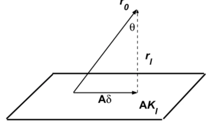
approximation s0, compute sl, the approximate solution for As = b, where sl ∈s0+Kl in such a way thatrl =b−Asl is orthogonal to AKl.
Sincesl ∈ s0+Kl we can writesl =s0+δ, δ ∈ Kl;thenrl =b−Asl = r0−Aδ. We obtainδin such a way thatrl is orthogonal toAKl. Geometrically,
Aδis the orthogonal projection ofr0inAKl, as shown in Figure 1.
AK
l
r
l
r
0
Aδ θ
Figure 1 – Orthogonal projection ofr0inAKl.
GMRES(m) is used in large scale problems. In this version, theGMRESproceeds
in cycles ofmiterations, see [14], [25]. Basically, the process begins with some
vectors0, and a fixed numbermof iterations are performed. Then, a new cycle
begins withsm as initial approximation and rm = b− Asm as initial residue.
Note that at each cycle an m-dimensional Krylov subspace is generated from
the initial residue, following the usualGMRESprocedure.
Whereas the restarted policy is computationally more feasible, convergence cannot be guaranteed in general, and stagnation becomes possible [11], [24], [28], [31] and [36]. A rather expensive remedy would be to monitor the eigenvalues of the Hessenberg matrices generated during theGMRES, [28]. Other schemes,
such as the one mentioned in [31], store some vectors created at the j-th cycle
and use them at the (j+1)-th cycle. We present a different strategy.
3 Stagnation
In this section we present a new strategy to generate an approximation to the new cycle that bypasses the stagnation of the method. We use the following notation:
r0j is the initial residue of the j-th cycle andrmj is the residual vector at the end
of this cycle.
Stagnation in GMRES(m) is usually describedas slowness in the decrease of the consecutive residual norms, krljk, l = 1,2,3, . . . ,m. However, a situa-tion where rmj andr01 are roughly linearly dependent could also be classified
as stagnant.
To prevent stagnation we need to control the cycles in such a way that it is possible to make a comparison between the norm of the last residue,krmjk, and
the norm of the initial residual vector of this cycle,kr0jk. Moreover, we need
to guarantee that the basis generated for the Krylov subspace in the(j+1)-th cycle is linearly independent with respect to the basis from the last cycles.
the progress of the process towards the solution will be very slow.
In Figure 1, we can observe that, given the projection property of GMRES,
if the cosine of the angle between the initial and final residual vectors is close to 1, then the norm of these residues are very close to each other so that there is an equivalence between the tests
krmjk/kr0jk ∼1 (2)
and
|cos(θj)| ∼1, (3)
whereθj is the angle between the vectorsr j 0 andr
j m.
We must also consider the possibility of linear dependence betweenrl 0, l =
1, . . . ,j −1 andrmj, wherer j
m is the last residue of the j-th cycle whereasr0l
is the initial residue of the l-th cycle. Nevertheless we decided to make the
comparison only betweenr01andrmj. Our stagnation criterion is based on
sim-plicity and heuristics. Simsim-plicity dictates a small number of angle comparisons; heuristics is justified as follows: comparison withr01is justified by the fact that,
empirically, the largest descent occurs during the first GMRES cycles. Angle
comparison withr0j is based on the heuristic assumption that once stagnation is
present it will always repeat itself; in other words, if the angle betweenr0j+1and r0j−1were small, stagnation would have already been discovered in the previous
cycle.
If a linear dependence betweenr01andrmj occurs, the Krylov subspace of the
cycle(j+1)would be close to the Krylov subspace generated in the first cycle. This would lead to the stagnation of the process. If this is the case, there is no equivalence between the tests (2) and (3), sincer01 andrmj belong to different
Krylov subspaces. Thus it is not possible to use the test with the norms of the residual vectors. Linear dependence can be detected testing the cosine of the angle between the residuesr01andrmj:
|cos(θj,1)| ∼1. (4)
In the strategies proposed in this work, the analysis will be always done at the end of each cycle, to reduce a too big computational costs. Stagnation will be declared when:
In case of stagnation, another initial approximation must be chosen for the new cycle. This new approximation is obtained using information generated during the process. However, it needs to be constructed in such a way to guarantee a reduction in the norm of the residual vector. The new strategy that is proposed generates an approximation for the (j +1)-th cycle using a hybrid scheme, based on the strategy proposed by Brezinski and Redivo-Zaglia in 1994, [3]. This hybrid scheme uses the approximationss01 andsmj which, in some sense,
take into account the information generated byGMRES(m). In this way, we are
trying to get out of a sequence which yields little decrease for the residuals. In what follows, we will briefly describe the scheme proposed in [3] for linear systems.
Consider the linear system of equations As =b. Once the approximationssˉ
andsˆare known, and the corresponding residues,rˉ =b−Asˉ andrˆ =b−Asˆ
are computed, the objective is to construct a new approximation as a linear combination ofsˉ andsˆ, s = αsˉ+βsˆ,with the aim of reducing the residual norm. As a simplifying tool in obtaining these parameters is to fixβ =1−α, and then the corresponding residuer will be given by
r =b−As=αrˉ+(1−α)rˆ.
Therefore our problem is reduced to findα ∈R, the least square solution for:
minαkrk =minαk(rˉ− ˆr)α+ ˆrk,
for which the optimalαis given by:
α = −(rˉ− ˆr)Trˆ/(rˉ− ˆr)T(rˉ− ˆr). (6)
The new approximation will bes =αsˉ+(1−α)sˆ, and the corresponding residue
isr =αrˉ+(1−α)ˆr.
Let us go back to the solution for As = b by the GMRES(m). Let s01 and smj denote the initial approximation of the whole process, and the last
approx-imation obtained after performing the m GMRESiterations of the j−th cycle,
respectively. The following safeguards are tested and the computation of the new approximation is done using the hybrid scheme, wheresˉ corresponds tos01
Strategy H: if j 6=1:
Safeguard 1: test the angleθj betweenr0j andrmj:
if|cos(θj)| ∼1, computes0j+1=αs01+(1−α)smj, withαgiven by (6).
Otherwise,
Safeguard 2: test the angleθj,1betweenr01andr j m:
if|cos(θj,1)| ∼1,then computes0j+1=αs01+(1−α)smj, withαgiven by (6).
if j =1:
Test the angleθ1betweenrm1 andr01:
if|cos(θ1)| ∼1, computesaas a random vector ands02=αsa+(1−α)sm1,
withαgiven by (6).
In the case j = 1, due to the orthogonality and minimization properties of GMRES, the vector calculated froms01is the same as the one encountered by the
hybrid process. Thus,s01 should be modified. We add that the corresponding
residual vectorra, related tosa, is normalized so as to guarantee the monotone
decrease of the residues.
In Figure 2 we depict the situation tested by Safeguard 2, when the decrease in the residual norm is sufficient, so that Safeguard 1 is not triggered. Thus,rmj
is necessarily much smaller thanr01.If indeed the angle between them is small, or close toπ,the residue formed by them will show a pronounced decrease in norm.
θ r
0 1
r
m j
r
0 j+1
Figure 2 – Safeguard 2: angle betweenr01andrmj, and residue obtained by the hybrid
scheme.
The hybrid scheme also presents the advantage of maintaining the minimization of the 2-norm ofr, as is the purpose ofGMRES(m). The important difference here
is that theGMRES(m) solves this problem in the Krylov subspace generated in
in the plane generated by vectors belonging to two different Krylov subspaces: the first Krylov subspace (K1) and the last Krylov subspace (Kj). Therefore
our scheme keeps some information about these two subspaces.
The hybrid vectors are used quite often. This idea is similar to theresidual smoothingused in [26], but in that case, it is used as a stopping criterion for
the Conjugate Gradient method; in [34] the authors compared the behavior of the smooth residue and the usual residue for the MRS, QMR and BCG methods. Hybrid preconditioners are used in [23] and [33]. We do not use the term “hybrid
GMRES” since in the literature it is sometimes used in other contexts, such as in
[18], [30]. So we are calling itGMRESH.
4 Numerical experiments withGMRESandGMRESH
We present two examples comparingGMRESandGMRESHfor 3×3 matrices.
Our procedure in this paper is the following: a hybrid restart is triggered in the first 5 occurrences of cos(θj) > 0.8 or cos(θj,1) > 0.8 and in the next 5
occurrences of cos(θj) > 0.9 or cos(θj,1) > 0.9. In all other next iterations,
the usualGMRES(m) is used. The point is that ifGMRESH(m) shows persistent
stagnation then further progress is not likely to occur.
Example 1. Zavorin [35] brings the linear system Ax =b:
A=
3.64347104554523 −1.30562625697964 2.12276233724947 3.81895186997748 −0.33626408416579 8.43952325416869 0.12754105943518 0.13002776444227 2.98820549610000
(7)
and
b=
−0.22385545043433
−0.30471918583417 0.92576182418211
.
For this example, the null vector was taken as the initial approximation. GMRES
was applied with restarts at each two iterations and it was allowed 100 cycles. The sequence of GMRES(2) residues is constant and equal to 1, showing the
stagnation of this method. For theGMRESH(2), the safeguards were triggered
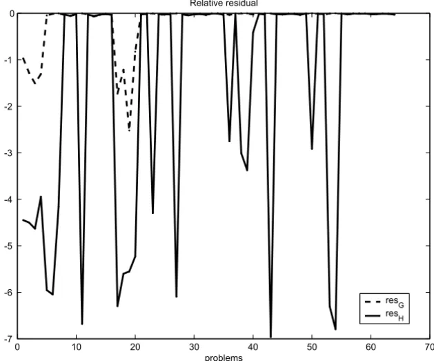
We also testedGMRES(2) andGMRESH(2) on 64 problems, which were created
as follows: consider the systems As = bi jl wherebi jl = b+vi jl,vi jl being a
vector in R3 with entries in [−0.1,0.1]. We used 4 points in each interval. Figure 3 shows the logarithmic relative error krendk/kr01k for each problem,
whererend is the last residue of the whole process. Although both methods
stagnated in some cases,GMRESH(2) shows a clear improvement.
0 10 20 30 40 50 60 70
-7 -6 -5 -4 -3 -2 -1 0
Relative residual
problems
res G res
H
Figure 3 – Logarithm of relative residual norms for the matrix (7). resG andresH
represent relative residues obtained byGMRES(2) andGMRESH(2), respectively.
Example 2. Embree [8] gives the linear system Ax =b:
A=
1 1 1 0 1 3 0 0 1
b=
2 −4
1
(8)
as an example whereGMRES(1) converges in three iterations but forGMRES(2)
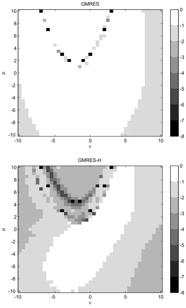
As=bνμ, where
r01=bνμ:=(ν, μ,1)T, ν, μ∈ [−10,10]
and 10−6was taken as precision. Figure 4 shows the logarithm of the relative
residual norms,(krendk/kr01k), ranging from 0 (white) to−8 (black). Actually,
some of theGMRESHrelative residues calculated were less than 10−16. We can
see that theGMRESH(2) relative residue is much smaller than theGMRES(2)
rel-ative residue in the vast majority of cases. Observing the size of the white region in both graphics, it is easy to conclude the better performance ofGMRESH(2).
We applied the deflatedGMRESDRmethod proposed by Morgan in [17] at the
resolution of the linear systems (7) and (8). The results were obtained using the programGMRESDR.m, kindly sent to us by R. Morgan (Baylor University). The
deflation of small eigenvalues can greatly improve the convergence of restarted
GMRES. This method is denoted byGMRESDR(m,k), wheremrepresents the
maximum dimension of the subspace andkbe the number of approximate
ein-genvectors (harmonic Ritz values) retained at a restart.
We observe that the matrices Aof these systems are not ill-conditioned. At
the resolution of system (7),GMRESDR(2,1) performed 69 inner iterations and
obtained relative residual of 5.8544e-005. Meanwhile,GMRESH(2) performed
19 inner iterations as seen before. Considering the 1681 problems of type (8), we had difficulties in runningGMRESDR(2,1) due to the ill conditioning introduced
by the change of the eigenvalue done by this method.
In conclusion, GMRESH(2) did a better job in avoiding stagnation in these
problems.
5 Numerical experiments
Here we apply theGMRES andGMRESH procedures, as linear solvers for the
inexact Newton method with a nonmonotone line search, [1], for solving a non-linear system
F(x)=0, F :Rn →Rn.
In the inexact Newton methods, [5], the sequencexk (called sequence of outer
iterations) is generated by
-8 -7 -6 -5 -4 -3 -2 -1 0 GMRES
ν
µ
-10 -5 0 5 10
-10 -8 -6 -4 -2 0 2 4 6 8 10
-8 -7 -6 -5 -4 -3 -2 -1 0 GMRES-H
ν
µ
-10 -5 0 5 10
-10 -8 -6 -4 -2 0 2 4 6 8 10
sk solves approximately the linear system J(xk)s = −F(xk), using this
stop-ping criterion:
kJ(xk)s+F(xk)k ≤ηkkF(xk)k, (9)
where J(.)is the Jacobian matrix, ηk ∈ (0,1]is the tolerance which is called the forcing term, [7].
In the line search procedure, it is needed the following parameters: σ ∈ (0, 1), ̺min and̺max such that 0 < ̺min < ̺max < 1 and the sequence {μk}
such thatμk >0 for allk =0,1,2, . . .and P∞
k=0μk =μ <∞.
Now we present the inexact Newton algorithm with the nonmonotone line search procedure. Let x0 ∈ Rn be an arbitrary initial approximation to the
solution for F(x)= 0. Givenxk ∈ Rn, and the toleranceε > 0, the steps to
obtain a new iteration xk+1are the following:
Algorithm 1. (Inexact Newton method with nonmonotone line search):
WhilekF(xk)k> ε,perform steps1to4:
Step 1:Chooseηk.
Step 2:Findsksuch thatkF(xk)+J(xk)skk ≤ηkkF(xk)k;
Step 3:Takeξ =1, computexaux =xk+skandF(xaux).
While
kF(xaux)k>[1−ξ σ]kF(xk)k +μk,
perform the steps3.1and3.2:
step 3.1: computeξnew ∈ [̺minξ, ̺maxξ];
step 3.2: setξ =ξnew and computexaux =xk+ξsk.
Step 4:Takeξk =ξ, computexk+1=xk+ξkskand updatek.
In the Step 1 we examine the following choices for the forcing term:
Constant (Cte): we choseηk =0.1;
EW1:ηk = k
F(xk)−F(xk−1)−J(xk−1)sk−1k
kF(xk−1)k (see Eisenstat and Walker [7]);
EW2: ηk = γ
kF(xk+1)k
kF(xk)k α
, γ ∈ [0,1], α ∈ (1,2] (see Eisenstat and
GLT:ηk = [1/(k+1)]ρcos2(φk) k F(xk)k
kF(xk−1)k
,ρ >1 and−π/2≤φk ≤0, (see
Gomes-Ruggiero et al. [10]).
The vectorskof the Step 2 is obtained byGMRES(m) andGMRESH(m).
The line search performed at Step 3 by Algorithm 1 follows the one proposed in [1] which is a nonmonotone strategy similar to the one introduced by Li and Fukushima, [12]. So, Algorithm 1 has global convergence [10]. Besides that, with the choicesEW1,EW2andGLTthe convergence rate is superlinear, [7], [10].
5.1 Implementation features
We give now more details about the implementation of the algorithms. The implementation details can be found in [32], pages 26 and 49. All the tests were performed in a Centrino Duo 1.6GHz with 1 GB Ram computer, using the software MatLab 6.1.
• Line search procedure (Step 3 of Algorithm1):
for the parameterσ, we took 1.d−04;
if the vectorxaux =xk+ξsk does not give an acceptable decrease in the
value of the function, then we compute the new step size asξnew =0.5ξ;
for the sequenceμk, we define: f ti p(0)= kF(x0)k,
f ti p(k)=min{kF(xk)k, f ti p(k−1)},ifkis a multiple of 3 and f ti p(k)= f ti p(k−1), otherwise;
then, we set:
μk =
f ti p(k) (k+1)1.1.
• The initial value and safeguards forη:
for all the choices forηkwe set the initial valueη0=0.1. For the choices EW1andEW2of [7] and for the choiceGLT, we takeηk =min{ηk, 0.1}
ifk ≤ 3, and ηk = min{ηk, 0.01} if k > 3. We also take ηk = 0.1
when φk > 0. At the final iterations we have adopted the safeguard
introduced in [22] which can be described as: since the linear model is
F(x)∼ F(xk)+J(xk)s, at the final iterations, we can have: kF(xk+1)k ∼
thatηkkF(xk)k ∼ ε whereε is the precision required for the nonlinear
system. A safeguard which represents these ideas is: ifηk ≤2ε then we
setηk =(0.8ε)kF(xk)k.
• Parameters choice forηk:
for the choiceEW2it was takenγ =1 andα =0.5(1+√5)and for the choiceGLTit was takenρ=1.1.
• Stopping criterion:
the process is finished successfully ifkF(xk)k ≤10−6andk<100.
• Restarts and the maximum number of iterations inGMRES(m):
we fix the restarts at eachm iterations, m = 30 or m = 50, allowing
initially a maximum of 100 cycles (100m iterations). This maximum
number is called here bymaxit and it is adjusted during the process.
This is the case, if the value of kFk increases, when F is computed
at the solution obtained after an inner iteration, before doing the line search. Also,maxitis adjusted when the number ofGMRES iterations
have exceeded a certain value. Indeed, maxit is computed according
to: if 1 < kF(xnew)k/kF(xold)k < 100, thenmaxitis fixed as 50; if
kF(xnew)k/kF(xold)k>100 or if the maximum number ofGMRES
itera-tions has been exceeded, thenmaxitis fixed as 30. We observe that this
procedure is repeated just in two consecutive iterations. After that, the value ofmaxitis taken as 100 again.
• StrategyH:
after eachGMRESiteration, a possible stagnation is detected by the tests (3)
and (4). Initially, we use 0.9 as a tolerance for the value of the cosine ofθj
orθj,1. If the hybrid scheme is triggered 5 times, we change this tolerance
to 0.8. In the case of the hybrid process be triggered at the beginning of 10 cycles, we stop the test as in Section 4.
5.2 A ray-tracing problem,[2]
We will present here a very simpliflied ray-tracing problem. First of all, let us represent the earth surface, as if it was two dimensional. Imagine that an acoustic wave transmiterSand a geophone receiverG, are located in two different
points on the earth surface. Each acoustic wave will cross a certain number of layers, under the surface, and when coming back, it will be captured by the geophone. Such layers considered elastic, isotropycs and homogeneous, compose the structure of the undersurfaces of the earth.
The problem that we are interested in, consists on determining the trajectory of a ray, when crossing the earth undersurface [13].
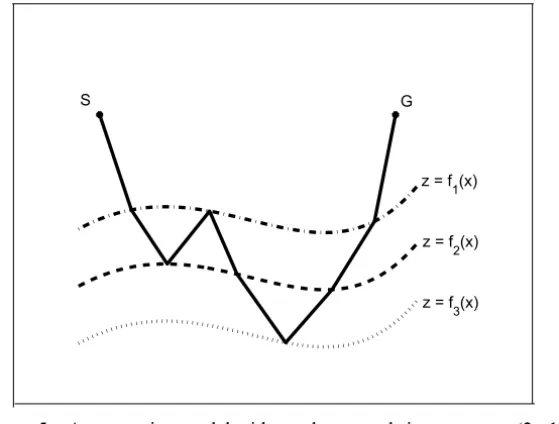
The interfaces between two consecutive layers, are defined as functions of the horizontal coordinatex.These functions are continuous and smooth – we will not consider the intersections between two consecutive interfaces. The functions will be represented byz = fi(x), i =1, . . . ,m,wheremcorresponds to the
number of interfaces andzdenotes the vertical coordinate.
S G
z = f
1(x)
z = f
2(x)
z = f3(x)
Figure 5 – A ray-tracing model with two layers and signaturea=(2, 1).
The number of times that a ray crosses the layer – downwards or upwards – in a layer between the interfaces fi and fi+1 will be denoted by (ai), i =
vectora =(a1, ∙ ∙ ∙ ,am−1)is calledthe signatureof the ray. For uniqueness,
we assume that all the downward crossings in a layer occur before those in the next layer, as in Figure 5.
Under these conditions, the rays must satisfy the Snell law, and so, they describe a straight line trajectory in each layer. Let the initial point S, the
end pointG on the earth surface, and the velocity of the ray in the j-th layer vj, j −1, . . . ,m−1,be given. The problem consists on finding the points Xk = (xk, fi k(xk)),for k = 1,2, . . . ,n that satisfy the Snell law in each
reflectorik. We will takeX0=SandXn+1=G. The dimension of the problem
is given by
n = 2 m−1 X
j=1
aj + 1.
The tangent vector to thek−th interface at the pointXk,will be calledτk,and
is defined byτk = (1, fi k′(xk). The Snell law is given by
1 vik
τkT (Xk−Xk−1)
kτkk kXk−Xk−1k =
1 vik+1
τkT (Xk+1−Xk)
kτkk kXk+1−Xkk
, (10)
where ||.|| denotes the Euclidean norm. Thus, using equation (10) for k =
1, . . . ,n we obtain a nonlinear system of equations with n equations and n
unknowns, given by
8(x)=0, (11)
with8 : Rn → Rn, 8(x) = (φ1(x), φ2(x),∙ ∙ ∙, φn(x))T and the functions
φk :Rn→R (k =1, ∙ ∙ ∙ , n) defined by
φk(x) = vik+1
(xk−xk−1)+ fi′k(xk) fik(xk)− fik−1(xk−1) h
(xk −xk−1)2+ fik(xk)− fik−1(xk−1)2 i1/2
−vik
(xk+1−xk)+ fi′k(xk) fik+1(xk+1)− fik(xk)
h
(xk+1−xk)2+ fik(xk+1)− fik(xk)
2i1/2 .
(12)
the result ofGMRES(left) andGMRESH(right). Columniterexrepresents the
total number of external iterations that were performed;iterin, the number
of inner iterations, that is, the number of iterations performed byGMRES(m) in
the whole process; the columnFevalrepresents the total number of function
evaluations needed during the whole process; finally,CPU timerepresents the
CPU time in seconds. The stopping criterion wask8k ≤10−5.
We observe that in this example the second safeguard in StrategyHwas never
triggered, while the first safeguard decreased considerably the number of inner iterations.
ηk iterex iterin Feval CPU time
Cte (6, 4) (7000, 4978) (7, 5) (135, 104)
EW1 (7, 4) (7840, 4054) (8, 5) (151, 84)
EW2 (7, 5) (7924, 4024) (8, 6) (153, 85)
GLT (7, 5) (7986, 4086) (8, 6) (155, 83)
Table 1 – Results for the ray-tracing problem withGMRES(30).
5.3 Boundary value problems
The general formulation of the boundary value problems solved in this work is findingu := [0, 1] × [0, 1] →R, such that, forλ∈R,
−1u+h(λ, u)= f(s,t), in , u(s,t)=0 on ∂. (13) The real valued functionh(λ,u), the different values for the parameterλand the function f define the different problems tested. All the problems were
dis-cretized using central differences on a grid withLinner points in each axis. The
discretized system obtained has L2equations and variables. In these problems
we work with grids ofL =63 and L =127 inner points. We now make a brief
description of the particular problems that were solved:
• Bratu problem: the functionh is given byh(λ,u) = λexp(u), and the function f(s,t)is constructed so that u∗(s,t)= 10st(1−s)(1−t)es4.5
• a convection-diffusion problem: in this problem, the functionh is given
byh(λ,u) = λu(us+ut), whereus andut denote the partial derivatives
of the functionu with respect tos andt, and again the function f(s,t) is defined so thatu∗(s,t) =10st(1−s)(1−t)es4.5 is the exact solution
for the problem. This is a problem considered difficult to solve [9], in particular for values ofλgreater than 50;
• a third problem: P3. This problem appears in the book of Briggs, Henson and McCormick [4], page 105. In this case,h(λ, u)is given byh(λ, u) = λueuand the function
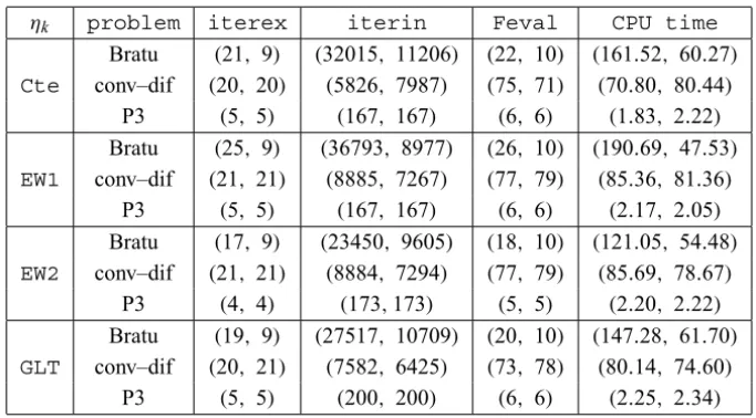
f(s,t)=((9π2+γe(x2−x3)sin(3πy))(x2−x3)+6x−2)sin(3πy). Table 2 shows the results of Newton-GMRES and Newton-GMRESHapplied
to the above problems, with: L = 63,n = 3969, x0 = (0, 0, . . . ,0)T and
λ = 100. This value forλwas chosen by the occurrence of stagnation. Each ordered pair should be read as in Table 1 anditerex,iterin,fevaland CPU timehave the same meaning as before.
ηk problem iterex iterin Feval CPU time
Bratu (21, 9) (32015, 11206) (22, 10) (161.52, 60.27)
Cte conv–dif (20, 20) (5826, 7987) (75, 71) (70.80, 80.44) P3 (5, 5) (167, 167) (6, 6) (1.83, 2.22) Bratu (25, 9) (36793, 8977) (26, 10) (190.69, 47.53)
EW1 conv–dif (21, 21) (8885, 7267) (77, 79) (85.36, 81.36) P3 (5, 5) (167, 167) (6, 6) (2.17, 2.05) Bratu (17, 9) (23450, 9605) (18, 10) (121.05, 54.48)
EW2 conv–dif (21, 21) (8884, 7294) (77, 79) (85.69, 78.67) P3 (4, 4) (173,173) (5, 5) (2.20, 2.22) Bratu (19, 9) (27517, 10709) (20, 10) (147.28, 61.70)
GLT conv–dif (20, 21) (7582, 6425) (73, 78) (80.14, 74.60) P3 (5, 5) (200, 200) (6, 6) (2.25, 2.34)
Table 2 – Results for the boundary value problems withGMRES(30).
For the Bratu problem,GMRESHshows a considerable decrease in the number
search was not triggered anditerexis slightly reduced. In the
convection-diffusion problem, the number of inner iterations was reduced with GMRES
in most of the cases. For this problem the Jacobian matrices are always ill-conditioned near the solution. The line search was activated several times, in-dicating stagnation coupled with insufficient decrease. For all the problems considered,iterexwas practically the same (or slighly better) usingGMRESH.
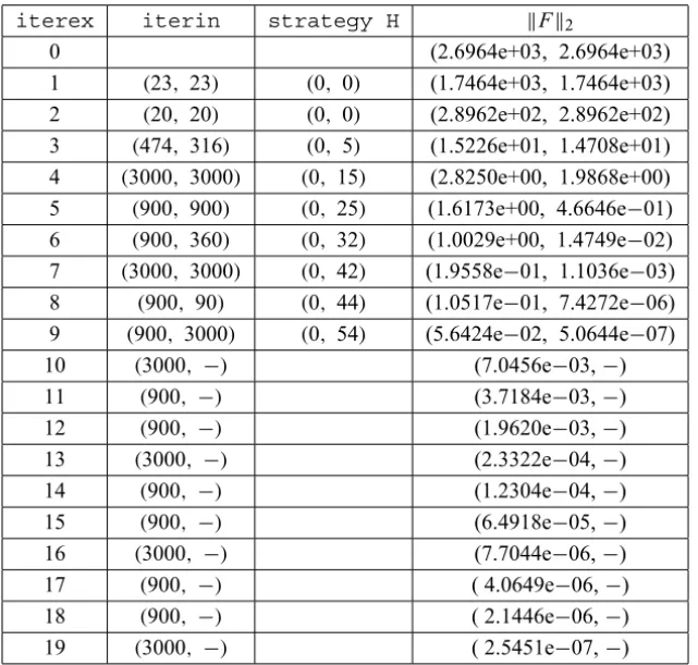
Problem P3 can be considered an easy problem with no ocurrence of stagnation. We show in Table 3, the performance of the Algorithm 1 with GLT choice
for the forcing term at the resolution of Bratu problem with λ = 100. Our purpose is to compare the number of inner iterations performed byGMRESand GMRESHat each outer iteration. We also show how many times the StrategyHis
triggered. We observe the ocurrence of stagnation at 4-th outer iteration. After this iteration, the strategyHwas triggered with a very good performance since
the number of inner iterations was extremely reduced and the convergence was accelerated.
We chose the Bratu and convection-diffusion problems to exploit other pa-rameters, such as the grid size L = 63 and L = 127. With these choices the
dimension of the nonlinear systems solved were 3969 and 16129, respectively.
We also implementedGMRES(m)withm =30 andm =50 for L = 63 and
m = 50 andm = 80 for L = 127. Table 4 shows the results for these
sys-tems. Observe that even with a very large dimension there was no difficulty for the Algorithm1to solve the corresponding nonlinear systems, in both cases: GMRES(m)andGMRESH(m). As before, for the Bratu problem,GMRESH(m)
shows a considerable decrease in the number of inner iterations, thus effectively mitigating the stagnation problem.
We also testedGMRESDR(30,5) at the resolution of the linear system
gener-ated at the first outer iteration of Algorithm1. It was slightly better than
GM-RESH(30) in solving Bratu problem but much better when solving convection-diffusion problem which has a very ill conditioned Jacobian matrix.
5.4 The performance profile of the methods
iterex iterin strategy H kFk2
0 (2.6964e+03, 2.6964e+03)
1 (23, 23) (0, 0) (1.7464e+03, 1.7464e+03) 2 (20, 20) (0, 0) (2.8962e+02, 2.8962e+02) 3 (474, 316) (0, 5) (1.5226e+01, 1.4708e+01) 4 (3000, 3000) (0, 15) (2.8250e+00, 1.9868e+00) 5 (900, 900) (0, 25) (1.6173e+00, 4.6646e−01) 6 (900, 360) (0, 32) (1.0029e+00, 1.4749e−02) 7 (3000, 3000) (0, 42) (1.9558e−01, 1.1036e−03) 8 (900, 90) (0, 44) (1.0517e−01, 7.4272e−06) 9 (900, 3000) (0, 54) (5.6424e−02, 5.0644e−07)
10 (3000, −) (7.0456e−03,−)
11 (900, −) (3.7184e−03,−)
12 (900, −) (1.9620e−03,−)
13 (3000, −) (2.3322e−04,−)
14 (900, −) (1.2304e−04,−)
15 (900, −) (6.4918e−05,−)
16 (3000, −) (7.7044e−06,−)
17 (900, −) ( 4.0649e−06,−)
18 (900, −) ( 2.1446e−06,−)
19 (3000, −) ( 2.5451e−07,−)
Table 3 – Performance ofGMRES(30)andGMRESH(30)at the linear systems in Bratu problem withλ=100.
measures, we can use, for instance, the number of iterations performed, the number of function evaluations, the CPU elapsed time, etc.
In this subsection we analyze the performance profile of the Algorithms
Newton-GMRES and Newton-GMRESH when applied to solve the boundary
value problems. A total of 18 problems were tested: Bratu, convection-diffusion and P3 with the following values forλ := 10, 25, 30, 50, 75 and 100. We compare the performance of this Algorithms using forηk only the choicesEW2
andGLT, in order to get an understandable figure. We used a grid withL =63
inner points andm = 30 because with these parameters the average behaviour
(L,m) ηk problem iterex iterin Feval CPU time EW2 Bratu (17, 9) (23450, 9605) (18, 10) (121, 54) (63, 30) conv–dif (21, 21) (8884, 7294) (77, 79) (86, 79)
GLT Bratu (19, 9) (27517, 10709) (20, 10) (147, 62)
conv–dif (20, 21) (7582, 6425) (73, 78) (80, 75)
EW2 Bratu (9, 7) (17772, 8171) (10, 8) (120, 58) (63, 50) conv–dif (19, 19) (2730, 2814) (73, 73) (53, 58)
GLT Bratu (9, 7) (17706, 5738) (10, 8) (100, 37)
conv–dif (19, 19) (2505, 2544) (71, 71) (51, 54)
EW2 Bratu (20, 9) (47171, 17991) (21, 10) (1093, 478) (127, 50) conv–dif (30, 21) (35090, 13730) (107, 79) (2108, 1144)
GLT Bratu (20, 8) (47415, 13746) (21, 9) (1092, 393)
conv–dif (20, 21) (8524, 13793) (72, 80) (1014, 1140)
EW2 Bratu (15, 8) (51705, 21510) (16, 9) (1713, 689) (127, 80) conv–dif (20, 20) (7256, 8596) (79, 79) (1011, 1084)
GLT Bratu (16, 8) (59862, 19930) (17, 9) (1903, 740)
conv–dif (19, 19) (6303, 7005) (70, 71) (975, 973)
Table 4 – Results for boundary value problems withL =63,GMRES(30),GMRES(50)
andL=127,GMRES(50),GMRES(80).
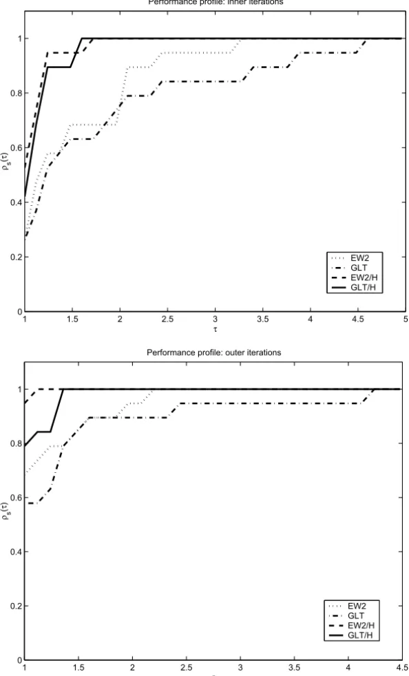
The measures used for comparison were the total numbers of inner and outer iterations. Note that in Figure 6 a higher curve means better performance. With respect to both measures, it is evident that the two Newton-GMRESH(NGH)
out-performed the two Newton-GMRES(NG) versions. In particular, the percentage
of problems solved with a small number of inner (resp. outer) iterations was roughly 43–53% against 30% (resp. 80–95% against 60–70%). It can be ob-served that NG versions solved some problems with a number of inner iterations 3 and 4 times greater than the minimum required to solve that problem with NGH versions. Thus the algorithm NG had a worse performance than the new version NGH. The strategies worked successfully.
6 Conclusions
1 1.5 2 2.5 3 3.5 4 4.5 5 0
0.2 0.4 0.6 0.8 1
Performance profile: inner iterations
τ
ρs
(
τ
)
EW2 GLT EW2/H GLT/H
1 1.5 2 2.5 3 3.5 4 4.5
0 0.2 0.4 0.6 0.8 1
Performance profile: outer iterations
τ
ρs
(
τ
)
EW2 GLT EW2/H GLT/H
of implementation, since it does not requires interfering in the inner procedure of the linear solverGMRES; (ii) it can be monitored at each iteration; (iii) from the
numerical results obtained, we can conclude that this strategy is efficient, either in the test for detecting the stagnation of the inner solver, or with respect to the safeguards triggered in this case. This conclusion can be seen in the solution of the ray-tracing problem, showed in Table 1, as well as in the solution of a bunch of boundary value problems whose performance profile is showed in Figure 6; (iv)GMRESH(m) is more efficient at the resolution of no ill conditioning
stag-nated systems. Maybe we can useGMRESH(m) together withGMRESDR(m,k)
to obtain a more efficient algorithm.
Acknowledgements. The authors are indebted to an anonymous referee for
the careful reading of this paper and also for the suggestions.
REFERENCES
[1] E.G. Birgin, N. Kreji´c and J.M. Martínez, Globally convergent inexact quasi-Newton methods for solving nonlinear systems. Numer. Algorithms,32(2003), 249–260.
[2] N. Bleistein,Mathematical Methods for Wave Phenomena. Academic Press, (1984).
[3] C. Brezinski and M. Redivo-Zaglia,Hybrid procedures for solving linear systems. Numer. Math.,67(1994), 1–19.
[4] W.L. Briggs, V.E. Henson and S.F. McCormick,A Multigrid Tutorial. Second Edition, SIAM, Philadelphia (1987).
[5] R.S. Dembo, S.C. Eisenstat and T. Steihaug,Inexact Newton methods. SIAM J. Numer. Anal.,
19(1982), 401–408.
[6] E.D. Dolan and J.J. Moré,Benchmarking optimization software with performance profile. Math. Program. ser.A91(2002), 201–213.
[7] S.C. Eisenstat and H.F. Walker,Choosing the forcing terms in inexact Newton method. SIAM J. Sci. Comput.,17(1996), 16–32.
[8] M. Embree,The tortoise and the hare restart GMRES. SIAM Review,45(2003), 259–266.
[9] M.A. Gomes–Ruggiero, D.N. Kozakevich and J.M. Martínez,A numerical study on large– scale nonlinear solvers. Comput. Math. Appl.,32(1996), 1–13.
[10] M.A. Gomes-Ruggiero, V.L. Rocha Lopes and J.V. Toledo-Benavides,A new choice for the forcing term and a global convergent inexact Newton method. Ann. Oper. Res.,157(2008),
[11] W. Joubert,On the convergence behavior of the restarted GMRES algorithm for solving nonsymmetric linear systems. Numer. Linear Algebra Appl.,1(1994), 427–447.
[12] D-H. Li and M. Fukushima, Derivative-free line search and global convergence of Broyden-like method for nonlinear equations. Optim. Methods Softw., 13(2000), 181–
201.
[13] H.B. Keller and D.J. Perozzi,Fast seismic ray-tracing. SIAM J. Appl. Math.,43(1983),
981–992.
[14] C.T. Kelley,Iterative Methods for Linear and Nonlinear Equations. SIAM, Philadelphia (1995).
[15] L.F. Mendonça and V.L. Rocha Lopes,Uma análise comparativa do desempenho de métodos quase–Newton na resolução de problemas em sísmica. Tema–SBMAC,5(2004), 107–116.
[16] R.B. Morgan,A restarted GMRES method augmented with eigenvectors. SIAM J. Matrix Anal. Appl.,16(1995), 1154–1171.
[17] R.B. Morgan,GMRES with deflated restarting. SIAM J. Sci. Comput.,24(2002), 20–37.
[18] N.M. Nachtigal, L. Reichel and L.N. Trefethen,A hybrid GMRES algorithm for nonsymmetric linear systems. SIAM J. Matrix Anal. Appl.,13(1992), 796–825.
[19] C.C. Paige and M.A. Saunders,Algorithm 583 LSQR: Sparse linear equations and least squares problems. ACM Trans. Math. Software,8(1982), 195–209.
[20] C.C. Paige and M.A. Saunders,LSQR: An algorithm for sparse linear equations and sparse least squares. ACM Trans. Math. Software,8(1982), 43–71.
[21] M. Parks, E. Sturler, G. Mackey, D.D. Johnson and S. Maiti,Recycling Krylov subspaces for sequences of linear systems. SIAM J. Sci. Comput.,28(2006), 1651–1674.
[22] M. Pernice and H. Walker,NITSOL: a Newton iterative solver for nonlinear systems. SIAM J. Sci. Comput.,19(1998), 302–318.
[23] Y. Saad,A flexible inner-outer preconditioned GMRES algorithm. SIAM J. Sci. Comput.,
14(1993), 461–469.
[24] Y. Saad,Iterative Methods for Sparse Linear Sistems. Second Edition, SIAM, Philadelphia (2003).
[25] Y. Saad and M.H. Schultz,GMRES: A generalized minimal residual algorithm for solving nonsymmetric linear systems. SIAM J. Sci. Comput.,7(1986), 856–869.
[26] W. Schonauer,Scientific Computing on Vector Computers. North-Holland, Amsterdam (1987).
[27] V. Simoncini,A new variant of restart GMRES(m). Numer. Linear Algebra Appl.,6(1999), 61–77.
[29] V. Simoncini and D.B. Szyld,Theory of inexact Krylov subspace methods and applications to scientific computing. SIAM J. Sci. Comput.,25(2003), 454–477.
[30] G. Starke and R.S. Varga,A hybrid Arnoldi–Faber iterative method for nonsymmetric systems of linear equations. Numer. Math.,64(1993), 213–240.
[31] E. de Sturler,Truncation strategies for optimal Krylov subspace methods. SIAM J. Numer. Anal.,36(1999), 864–889.
[32] J.V. Toledo-Benavides,A globally convergent Newton-GMRES method with a new choice for the forcing term and some strategies to improve GMRES(m). PhD Thesis, T/UNICAMP T575m, (2005).
[33] H.A. Van der Vorst and C. Vuik,GMRESR: a family of nested GMRES methods. Num. Linear Algebra Appl.,1(1994), 369–386.
[34] H.F. Walker and L. Zhou,Residual smoothing techniques for iterative methods. SIAM J. Sci. Comput.,15(1994), 297–312.
[35] I. Zavorin,Spectral factorization of the Krylov matrix and convergence of GMRES. UMIACS Technical Report CS-TR-4309, University of Maryland, College Park (2002).
[36] I. Zavorin, D.P. O’Leary and H. Elman,Complete stagnation of GMRES. Lin. Algebra Appl.,