ISSN 0101-8205 www.scielo.br/cam
Residual iterative schemes for large-scale
nonsymmetric positive definite linear systems
WILLIAM LA CRUZ1∗ and MARCOS RAYDAN2∗∗
1Dpto. de Electrónica, Computación y Control, Escuela de Ingeniería Eléctrica Facultad de Ingeniería, Universidad Central de Venezuela
Caracas 1051-DF, Venezuela
2Dpto. de Computación, Facultad de Ciencias, Universidad Central de Venezuela Ap. 47002, Caracas 1041-A, Venezuela
E-mails: [email protected] / [email protected]
Abstract. A new iterative scheme that uses the residual vector as search direction is proposed and analyzed for solving large-scale nonsymmetric linear systems, whose matrix has a positive (or negative) definite symmetric part. It is closely related to Richardson’s method, although the stepsize and some other new features are inspired by the success of recently proposed residual methods for nonlinear systems. Numerical experiments are included to show that, without precon-ditioning, the proposed scheme outperforms some recently proposed variations on Richardson’s method, and competes with well-known and well-established Krylov subspace methods: GMRES and BiCGSTAB. Our computational experiments also show that, in the presence of suitable precon-ditioning strategies, residual iterative methods can be competitive, and sometimes advantageous, when compared with Krylov subspace methods.
Mathematical subject classification: 65F10, 65F25, 49M07.
Key words:linear systems, Richardson’s method, Krylov subspace methods, spectral gradient method.
#722/07. Received: 08/V/07. Accepted: 28/XI/07.
∗This author was supported by CDCH project PI-08-14-5463-2004 and Fonacit
UCV-PROJECT 97-003769.
∗∗This author was supported by the Graduate Program in Computer Science at UCV and
1 Introduction
We are interested in solving linear systems of equations,
Ax =b, (1)
where A ∈Rn×n is not symmetric,(A+ AT)is positive (or negative) definite, b ∈ Rn, and n is large. This kind of linear systems arise in many areas of
scientific computing. For example, when discretizing the two point boundary value problems or the partial differential equations that frequently appear in oil-reservoir engineering, in weather forecasting, or in electronic device modelling among others, linear systems like (1) need to be solved (see, e.g., [1, 16]).
The well-known Richardson’s method (also known as Chebyshev method) and its variations are characterized by using the residual vector,r(x)=b− Ax, as search direction to solve linear systems iteratively (see, e.g., [7, 11, 12, 24, 26]). In general, these variations of Richardson’s method have not been considered to be competitive with Krylov subspace methods, which represent nowadays the best-known options for solving (1), specially when combined with suitable preconditioning strategies. For a review on Richardson’s method and variations see [8, 29, 30].
Nevertheless, from a different perspective, solving linear systems of equations can be seen as a particular (although very special) case of solving nonlinear systems of equations. For nonlinear systems, some new iterative schemes have recently been presented that use in a systematic way the residual vectors as search directions [19, 20]. These low-memory ideas become effective, and competitive with Newton-Krylov ([3, 9, 10, 18]) schemes for large-scale nonlinear systems, when the step lengths are chosen in a suitable way.
In this work we combine and adapt, for linear systems, the ideas introduced in [19, 20] for the nonlinear case. To be precise, we present in Section 2 a scheme that takes advantage of the method presented in [19] for choosing the direction, plus or minus the residual, depending on the sign of a Rayleigh quotient closely related to the step length. It also takes advantage of the new globalization strategy proposed and analyzed in [20] that allows the norm of the residual to decrease non monotonically and still guarantees convergence.
as search direction, then it can be viewed as a new variant of the well-known Richardson’s method. However, there are significant new features. The most important is the use of the spectral steplength choice, also known as the Barzilai-Borwein choice, ([2, 13, 17, 22]) that has proved to yield fast local convergence for the solution of nonlinear optimization problems ([4, 5, 6, 15, 23]). However, this special choice of step size cannot guarantee global convergence by itself, as it usually happens with other variations (see, e.g., [7, 11, 12, 24, 26]). For that, we combine its use with a tolerant globalization strategy, that represents the second new feature. In section 3 we present a preliminary numerical experimentation to compare the proposed scheme with some variations on Richardson’s method, and also with well-known and well-established Krylov subspace methods: GMRES and BiCGSTAB, with and without preconditioning. In section 4 we present some concluding remarks.
2 General algorithm and convergence
We now present our general algorithm for solving the minimization problem
min
x∈Rn f(x)≡ kg(x)k
2
,
where
g(x)= Ax−b, (2)
andk ∙ kdenotes, throughout this work, the Euclidian norm. The new algorithm generates the iterates using plus or minus the residual vector as search direc-tion, and a spectral steplength closely related to the Barzilai-Borwein choice of steplength [2], as follows
xk+1=xk+sgn(βk)(1/βk−1)rk,
whereβk = (rktArk)/(rktrk), andrk = b− Axk = −g(xk) is the residual
vec-tor at xk. The use of the this steplength is inspired by the success obtained
recently for solving nonlinear systems of equations [19, 20]. Properties of the spectral step length, αk+1 = (rktrk)/(rktArk), for the minimization of convex
To guarantee convergence, from any initial guess x0 and any positive initial steplength 1/β0, the nonmonotone line search condition
f(xk+1)≤ f(xk)+ηk−γ λ2kkg(xk)k2, (3)
needs to be enforced at everyk, for a 0< λk ≤1. Obtainingλkvia a backtracking
process to force (3) represents a globalization strategy that is inspired by the proposition presented in [20], and requires some given parameters: {ηk},γ, and
σmin < σmax. Let us assume that{ηk}is a given sequence such thatηk >0 for
allk ∈N(the set of natural numbers) and
∞
X
k=0
ηk =η <∞. (4)
Let us also assume thatγ ∈(0,1)and 0< σmin< σmax<1. Algorithm 2.1. Residual Algorithm1(RA1)
Given: x0 ∈ Rn, α
0 > 0, γ ∈ (0,1), 0 < σmin < σmax < 1, {ηk}k∈N such
that (4) holds. Setr0=b−Ax0, andk=0;
Step 1. Ifrk =0, stop the process (successfully);
Step 2. Setβk =(rktArk)/(rktrk);
Step 3. Ifβk =0, stop the process (unsuccessfully);
Step 4. (Backtracking process) Setλ←1;
Step 5. Ifkrk−sgn(βk)(λ/αk)Arkk2≤ krkk2+ηk−γ λ2krkk2go to Step 7;
Step 6. Chooseσ ∈ [σmin, σmax], setλ←σ λ, and go to Step 5;
Step 7. Setλk =λ,xk+1=xk+sgn(βk)(λ/αk)rk, andrk+1=rk−sgn(βk)(λ/
αk)Ark;
Step 8. Setαk+1= |βk|,k=k+1 and go to Step 1.
Remark 2.1. In practice, the parameters associated with the line search strategy are chosen to reduce the number of backtrackings as much as possible while keeping the convergence properties of the method. For example, the parameter
large number whenk =0 and then it is reduced as slow as possible making sure that (4) holds (e.g.,ηk =104(1−10−6)k). Finallyσmin < σmax are chosen as classical safeguard parameters in the line search process (e.g., σmin = 0.1 and
σmax=0.5).
Remark 2.2. For allk ∈N, the following properties can be easily established:
(i) g(xk+1)=g(xk)−sgn(βk)(λk/αk)Ag(xk).
(ii) dk =sgn(βk)(1/αk)rk = −sgn(βk)(1/αk)g(xk).
(iii) f(xk+λdk)= krk −sgn(βk)(λ/αk)Arkk2.
(iv) krk−(λ/αk)sgn(βk)Arkk2 ≤ krkk2+ηk−γ λ2krkk2.
In order to present some convergence analysis for Algorithm 2.1, we first need some technical results.
Proposition 2.1. Let {xk}k∈N be the sequence generated by Algorithm 2.1.
Then, dkis a descent direction for the function f , for all k∈N.
Proof. Since∇f(x)=2Atg(x), then we can write
∇ f(xk)tdk = 2(g(xk)tA)(−sgn(βk)(1/αk)g(xk))
= −2(g(xk)tAg(xk))sgn(βk)(1/αk)
= −2(βk(g(xk)tg(xk)))sgn(βk)(1/αk)
= −2(|βk|/αk)kg(xk)k2<0, fork ∈N.
This completes the proof.
By Proposition 2.1 it is clear that Algorithm 2.1 can be viewed as an iterative process for finding stationary points of f. In that sense, the convergence analysis for Algorithm 2.1 consists in proving that the sequence of iterates{xk}k∈Nis such
that limk→∞∇f(xk)=0.
First we need to establish that Algorithm 2.1 is well defined.
Proof. Sinceηk >0, then by the continuity of f(x), the condition
f(xk+λdk)≤ f(xk)+ηk−γ λ2kg(xk)k2,
is equivalent to
krk−(λ/αk)sgn(βk)Arkk2≤ krkk2+ηk −γ λ2krkk2,
that holds forλ >0 sufficiently small.
Our next result guarantees that the whole sequence of iterates generated by Algorithm 2.1 is contained in a subset ofRn.
Proposition 2.3. The sequence {xk}k∈N generated by Algorithm 2.1 is
con-tained in the set
80=
x ∈Rn :0≤ f(x)≤ f(x0)+η . (5)
Proof. Clearly f(xk)≥ 0 fork ∈N. Hence, it suffices to prove that f(xk)≤
f(x0)+ηfork ∈N. For that we first prove by induction that
f(xk)≤ f(x0)+ k−1
X
i=0
ηi. (6)
Equation (6) holds fork =1. Indeed, sinceλ1satisfies (3) then f(x1)≤ f(x0)+η0.
Let us suppose that (6) holds fork−1 wherek ≥2. We will show that (6) holds fork. Using (3) and (6) we obtain
f(xk)≤ f(xk−1)+ηk−1≤ f(x0)+
k−2
X
i=0
ηi +ηk−1= f(x0)+
k−1
X
i=0
ηi,
which proves that (6) holds fork ≥2. Finally, using (4) and (6) it follows that, fork ≥0:
f(xk+1)≤ f(x0)+
k X
i=0
ηi ≤ f(x0)+η,
and the result is established.
Proposition 2.4. Let {ak}k∈N and {bk}k∈N be sequences of positive numbers
satisfying
ak+1≤(1+bk)ak+bk and ∞
X
k=0
bk <∞.
Then,{ak}k∈Nconverges.
Proposition 2.5. If{xk}k∈Nis the sequence generated by Algorithm2.1, then
∞
X
k=0
kxk+1−xkk2<∞, (7)
and
lim
k→∞λkkg(xk)k =0. (8)
Proof. Using Proposition 2.3 and the fact that 80 is clearly bounded,
{kg(xk)k}k∈N is also bounded. Since kxk+1 −xkk = λkkg(xk)k, then using
(3) we have that
kxk+1−xkk2=λ2kkg(xk)k2≤
ηk
γ +
1
γ f(xk)− f(xk+1)
. (9)
Sinceηksatisfies (4), adding in both sides of (9) it follows that
∞
X
k=0
kxk+1−xkk2 ≤
1
γ
∞
X
k=0
ηk+
1
γ
∞
X
k=0
f(xk)− f(xk+1)
≤ η+ f(x0)
γ <∞,
which implies that
lim
k→∞kxk+1−xkk =0,
and so
lim
k→∞λkkg(xk)k =0.
Hence, the proof is complete.
Proposition 2.6. If{xk}k∈Nis the sequence generated by Algorithm2.1, then
Proof. Since f(xk) ≥ 0 and(1+ηk) ≥ 1, for allk ∈ N, then using (3) we
have that
f(xk+1)≤ f(xk)+ηk ≤(1+ηk)f(xk)+ηk.
Settingak = f(xk)andbk =ηk, then it can also be written as
ak+1≤(1+bk)ak+bk,
andP∞
k=0bk < η < ∞. Therefore, by Proposition 2.4, the sequence{ak}k∈N
converges, i.e., the sequence {f(xk)}k∈N converges. Finally, since f(x) = kg(x)k2, then the sequence{kg(x
k)k}k∈Nconverges.
We now present the main convergence result of this section. Theorem 2.1 shows that either the process terminates at a solution or it produces a sequence
{rk}k∈Nfor which limk→∞rktArk =0.
Theorem 2.1. Algorithm2.1terminates at a finite iteration i where ri =0, or
it generates a sequence{rk}k∈Nsuch that
lim
k→∞r t
kArk =0.
Proof. Let us assume that Algorithm 2.1 does not terminate at a finite iteration. By continuity, it suffices to show that any accumulation pointxˉ of the sequence
{xk}k∈N satisfies g(xˉ)tAg(xˉ) = 0. Let xˉ be a accumulation point of{xk}k∈N.
Then, there exists an infinite set of indicesR⊂Nsuch that limk→∞,k∈Rxk = ˉx. From Proposition 2.5 we have that
lim
k→∞λkkg(xk)k =0
that holds if
lim
k→∞kg(xk)k =0, (10)
or if
lim inf
k→∞ λk =0. (11)
If (10) holds, the result follows immediately.
Let us assume that (11) holds. Then, there exists an infinite set of indices K = {k1,k2,k3, . . .} ⊆Nsuch that
lim
IfR∩K = ∅, then by Proposition 2.5
lim
k→∞,k∈Rkg(xk)k =0.
Therefore, the thesis of the theorem is established.
Without loss of generality, we can assume that K ⊆ R. By the way λkj is
chosen in Algorithm 2.1, there exists an index ˉjsufficiently large such that for all j ≥ ˉj, there existsρkj (0< σmin ≤ρkj ≤σmax) for whichλ=λkj/ρkj does
not satisfy condition (3), i.e.,
f xkj + λkj
ρkj
dkj !
> f(xkj)+ηkj −γ λ2
kj
ρk2 j
kg(xkj)k
2
≥ f(xkj)−γ λ2k
j
ρk2 j
kg(xkj)k
2
.
Hence,
f
xkj +
λk j
ρk jdkj
− f xkj
λkj/ρkj
>−γλkj ρkj
kg(xkj)k
2
≥ −γ λkj σmin
kg(xkj)k
2
.
By the Mean Value Theorem it follows that
∇f xkj +tkjdkj t
dkj >−γ λkj
σmin
kg(xkj)k
2
, for j ≥ ˉj, (12)
wheretkj ∈ [0, λkj/ρkj] tends to zero when j → ∞. By continuity and the
definitions ofβkanddk, we obtain
lim
j→∞dkj = −sgn
g(xˉ)tAg(xˉ)
g(xˉ)tg(xˉ)
(1/α)ˉ g(xˉ), (13)
where αˉ = limk→∞,k∈Kαk. We can assume that α >ˉ 0. If αˉ = 0, then
by the definition of theαk, the thesis of the theorem is established. Setting ˉ
d =limj→∞dkj and noticing that(xkj+tkjdkj)→ ˉxwhen j → ∞, then taking
limits in (12) we have that
∇f(xˉ)tdˉ≥0. (14)
Since∇f(xˉ)tdˉ =2g(xˉ)tAd,ˉ α >ˉ 0, and∇f(xˉ)tdˉ <0, then by (13) and (14)
we obtain
g(xˉ)tAg(xˉ)=0.
Theorem 2.1 guarantees that Algorithm 2.1 converges to a solution of (1) whenever the Rayleigh quotient of A,
c(x)= x tAx
xtx , x 6=0, (15)
satisfies that|c(rk)|>0, for k ≥ 1. If the matrix Ais indefinite, then it could
happen that Algorithm 2.1 generates a sequence{rk}k∈N that converges to the
residualrˉsuch thatrˉtArˉ =0 andrˉ6=0.
In our next result, we show the convergence of the algorithm when the sym-metric part of A, As = (At + A)/2, is positive definite, that appears in many
different applications. Of course, similar properties will hold whenAsis negative
definite.
Theorem 2.2. If the matrix As is positive definite, then Algorithm 2.1
termi-nates at a finite iteration i where ri =0, or it generates a sequence{rk}k∈Nsuch
that
lim
k→∞rk =0.
Proof. Since Asis positive definite,rktArk =rktASrk >0,rk 6=0, for allk ∈N.
Then, by the Theorem 2.1 the Algorithm 2.1 terminates at a finite iteration i whereri =0, or it generates a sequence{rk}k∈Nsuch that limk→∞rk =0.
To be precise, the next proposition shows that if As is positive definite, then in
Algorithm 2.1 it holds thatβk >0 anddk =(1/αk)rk, for allk∈N.
Proposition 2.7. Let the matrix Asbe positive definite, and letαminandαmaxbe the smallest and the largest eigenvalues of As, respectively. Then the sequences {βk}k∈N and{dk}k∈N, generated by Algorithm2.1 satisfy that dk = (1/αk)rk,
for k ∈N.
Proof. It is well-known that the Rayleigh quotient ofAsatisfies, for anyx 6=0,
0< αmin ≤c(x)≤αmax. (16)
By the definition ofβkwe have that
Moreover, sinceβk >0 fork ≥0, then
dk =sgn(βk)(1/αk)rk =(1/αk)rk, for k ≥0.
Proposition 2.7 guarantees that the choice dk = (1/αk)rk is a descent
di-rection, when As is positive definite. This yields a simplified version of the
algorithm for solving linear systems when the matrix has positive (or negative) definite symmetric part. This simplified version of the algorithm will be re-ferred, throughout the rest of this document, as the Residual Algorithm 2 (RA2), for whichβk =αk+1=(rktArk)/(rktrk)and sgn(βk)=1 for allk.
Remark 2.3.
(i) AlgorithmRA2is well defined.
(ii) The sequence{xk}k∈Ngenerated by AlgorithmRA2is contained in80.
(iii) Sinceαk+1=c(rk)andc(x)satisfies (16), then
0< αmin≤αk ≤αmax, for k ≥1. (17)
Moreover,
0< (λk/αk)≤σmaxα−min1, for k ≥1.
(iv) Since AlgorithmRA2is a simplified version of Algorithm 2.1 whenAs is
positive definite, then its convergence is established by Theorem 2.2.
3 Numerical experiments
We report on some numerical experiments that illustrate the performance of algorithmRA2, presented and analyzed previously, for solving nonsymmetric and positive (or negative) definite linear systems. In all experiments, computing was done on a Pentium IV at 3.0 GHz with MATLAB 6.0, and we stop the iterations when
krkk
kbk ≤ε, (18)
As we mentioned in the introduction, our proposal can be viewed as a new variant of the well-known Richardson’s method, with some new features. First, we will compare the behavior of algorithmRA2with two different variations of Richardson’s method, whose general iterative step from a givenx0is given by
xk+1=xk+λkrk,
where the residual vectors can be obtained recursively as
rk+1=rk −λArk.
It is well-known that if we choose the steplengths as the inverse of the eigenvalues ofA(i.e.,λk =λi−1for 1≤i ≤n), then in exact arithmetic the process
termi-nates at the solution in at most n iterations (see [8] and references therein). Due to roundoff errors, in practice, this process is repeated cyclically (i.e.,
λk = λ−i 1mod n for all k ≥ n). In our results, this cyclic scheme will be
re-ported as theideal Richardson’s method.
A recent variation on Richardson’s method that has optimal properties con-cerning the norm of the residual, is discussed by Brezinski [7] and chooses the steplength as follows:
λk =
rkTwk
wkTwk
, (19)
wherewk = Ark. This option will be referred in our results as the Optimal
Richardson’s Method(ORM).
For our first experiment, we setn = 100, b = rand(n,1), ε = 10−16, and the matrix
A= −Galler y(′lesp′,n).
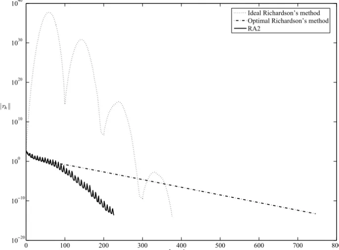
The results for this experiment are shown in Figure 1. We observe that the ideal Richardson’s method is numerically unstable and requires several cycles to ter-minate the process. The ORM has a monotone behavior and it is numerically stable, but requires more iterations than theRA2algorithm to reach the same ac-curacy. It is also worth noticing the nonmonotone behavior of theRA2algorithm that accounts for the fast convergence.
0 100 200 300 400 500 600 700 800 1020
1010 100 1010 1020 1030 1040
Iterations rk
Ideal Richardson’s method Optimal Richardson’s method RA2
Figure 1 – Behavior of the ideal and the optimal Richadson’s method when compared with theRA2algorithm for A= −Galler y(′lesp′,100).
Krylov iterative methods for solving large-scale non symmetric linear systems (see, e.g., [27, 29]). Therefore, we compare the performance of algorithmRA2 with these two methods, and also with ORM, without preconditioning and also taking advantage of two classical preconditioning strategies of general use: In-complete LU (ILU) and SSOR. For the preconditioned version of ORM [7], the search direction is given byzk =Crk, whereC is the preconditioning matrix;
and the steplength is given by (19) where nowwk = Azk. In the preconditioned
version ofRA2the residual is redefined asrk =C(b−Axk)for allk ≥0, where
once againCis the preconditioning matrix.
all considered methods we use the vectorx0 =0 as the initial guess. For algo-rithmRA2we use the following parameters: α0 = kbk,γ =10−4,σmin=0.1,
σmax =0.5, andηk =104 1−10−6 k
. For choosing a newλat Step 4, we use the following procedure, described in [20]: given the currentλc>0, we set the
newλ >0 as
λ=
σminλc, ifλt < σminλc;
σmaxλc, ifλt > σmaxλc;
λt, otherwise;
where
λt =
λ2cf(xk)
f(xk+λcd)+(2λc−1)f(xk)
.
In the following tables, the process is stopped when (18) is attained, but it can also be stopped prematurely for different reasons. We report the different possible failures observed with different symbols as follows:
* : The method reaches the maximum (20000) number of iterations.
** : The method stagnates (three consecutive iterates are exactly the same).
*** : Overflow is observed while computing one of the internal scalars.
For our second experiment we consider a set of 10 test matrices, described in Table 1, and we set the right hand side vectorb = (1,1, . . . ,1)t ∈ Rn. In Table 1 we report the problem number (M), a brief description of the matrix, and the MATLAB commands to generate it.
We summarize on Table 2 the behavior of GMRES(20), GMRES(40), BICGSTAB, ORM, and RA2 without preconditioning. We have chosen ε =
M Description MATLAB Commands
1 Sparse adjacency matrix from NASA airfoil.
MATLAB demo: airfoil
2 Singular Toeplitz lower Hessenberg matrix
A=gallery(’chow’,n,1,1)
3 Circulant matrix A=gallery(’circul’,v), wherev ∈ Rn
is such that
vi =
10−6, i =1,
1, i =n/2,
−1, i =n,
0, otherwise.
4 Diagonally dominant, ill condi-tioned, tridiagonal matrix
A=gallery(’dorr’,n,1)
5 Perturbed Jordan block A=gallery(’forsythe’,n,-1,2) 6 Matrix whose eigenvalues lie on a
vertical line in the complex plane
A=gallery(’hanowa’,n,n)
7 Jordan block A=gallery(’jordbloc’,n,2)
8 Tridiagonal matrix with real sensi-tive eigenvalues
A = -gallery(’lesp’,n)
9 Pentadiagonal Toeplitz matrix A=gallery(’toeppen’,n,1,10,n,-10,-1) 10 Upper triangular matrix discussed by
Wilkinson and others
A=gallery(’triw’,n,-0.5,2)
Table 1 – First set of test matrices.
In Tables 3 and 4 we report the results for the matrices 4, 5, 6, 7, 8 and 9, when we use the following two preconditioning strategies.
(A) Incomplete LU factorization with drop tolerance
The preconditioning matrix is obtained, in MATLAB, with the command
[L,U]= luinc(A,0.5).
(B) The SSOR preconditioning strategy The preconditioning matrix is given by
where−E is the strict lower triangular part of A,−F is the strict upper triangular part ofA, and Dis the diagonal part of A. We takeω=1.
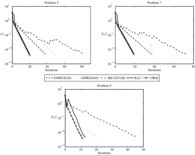
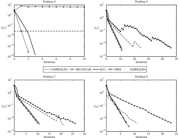
In this case, we setε=5×10⁻¹⁵in (18) for stopping the iterations. In Figure 2 we show the behavior of all considered methods when using preconditioning strategy (A) for problems 5, 7 and 8; and in Figure 3 for problems 4, 5, 7 and 8 when using preconditioning strategy (B).
Table 2 – GMRES(20), GMRES(40), BICGSTAB,RA2, and ORM without precondi-tioning.
GMRES(20) GMRES(40) BICGSTAB RA2 ORM
M n Iter T Iter T Iter T Iter T Iter T
4 50000 * * * * * * 3 0.088 2 0.094
5 500000 38 59.500 48 97.859 81 37.781 20 4.625 20 5.469 6 500000 1 0.715 1 0.715 1 0.715 2 0.547 1 0.438 7 500000 37 57.500 38 84.375 72 33.469 20 4.641 19 5.453 8 500000 21 34.359 21 35.438 46 22.969 10 2.516 11 3.391 9 500000 2 2.341 2 2.859 3 2.250 2 0.719 2 0.922
Table 3 – GMRES(20), GMRES(40), BICGSTAB,RA2, and ORM with precondition-ing (A).
Table 4 – GMRES(20), GMRES(40), BICGSTAB,RA2, and ORM with precondition-ing (B).
0 20 40 60 80 1015
1010 105 100 105
Iterations
||rk||
Problem 5
GMRES(20) GMRES(40) BICGSTAB RA2 ORM
0 20 40 60 80 1015
1010 105 100 105
Iterations
||rk||
Problem 7
0 10 20 30 40 50 1015
1010 105 100 105
Iterations
||rk||
Problem 8
Figure 2 – Behavior of all methods when using preconditioning techniques (A).
hand side vectorb=(1,1, . . . ,1)t and the matrix
A=
a11 −1
1 a22 −1
. .. ... . ..
1 an−1,n−1 −1
1 ann
0 2 4 6 8 10 1020
1015 1010 105 100 105
Iterations
||rk||
Problem 4
0 10 20 30 40 50 1015
1010 105 100 105
Iterations
||rk||
Problem 5
0 5 10 15 20 25 30 1015
1010 105 100 105
Iterations
||rk||
Problem 7
0 5 10 15 20 25 1015
1010 105 100 105
Iterations
||rk||
Problem 8 GMRES(20) BICGSTAB RA2 ORM GMRES(40)
Figure 3 – Behavior of all methods when using preconditioning techniques (B).
wheren =10000,aii =3+(i−1) αmaxn−−13
, fori =1, . . . ,n, andαmax≥ 3. It is clear that the symmetric part ofAis a diagonal matrix whose eigenvalues are
μi =aii, fori =1, . . . ,n. We consider the following three cases: (i)αmax=10, (ii)αmax=1000, and (iii)αmax=10000. We have chosenε =10−15in (18) for stopping the iterations.
Figure 4 shows the behavior of RA2, with and without preconditioning, for the system Ax = b and each one of the cases (i), (ii) and (iii). We clearly observe that clustering the eigenvalues of the symmetric part drastically reduce the number of required iterations. We can also observe that preconditioning (A) was more effective on cases (ii) and (iii), since the eigenvalues in case (i) are already clustered. A similar behavior is observed when the clustering effect is applied to ORM.
0 100 200 300 400 500 600 700 800 900 1000 1100 1200 1300 1400 1500 1600 10−20
10−10 100 1010
Iterations
rk
RA2 without preconditioning
(i) (ii) (iii)
0 1 2 3 4 5 6 7 8 9 10 11 12 13 14 15 16 17 18 19 20 21 22 23 24 25 10−20
10−10 100 1010
Iterations
rk
RA2 with preconditioning (A)
(i) (ii) (iii)
Figure 4 – Behavior ofRA2for solving Ax = bwhen clustering the eigenvalues for
each one of the cases (i), (ii) and (iii).
discretization of
−∇2u+γ (xux +yuy)+βu= f, (20)
on the unit square, with homogeneous Dirichlet boundary conditions,u = 0, on the border of the region. We set the parameters γ = 7100 andβ = 100 to guarantee that the symmetric part of the matrix is positive definite. The discretization grid has 71 internal nodes per axis producing an n ×n matrix wheren = 5041. The right hand side vector is chosen such that the solution vector isx =(1,1. . . ,1)t. Once again we compare GMRES(20), GMRES(40),
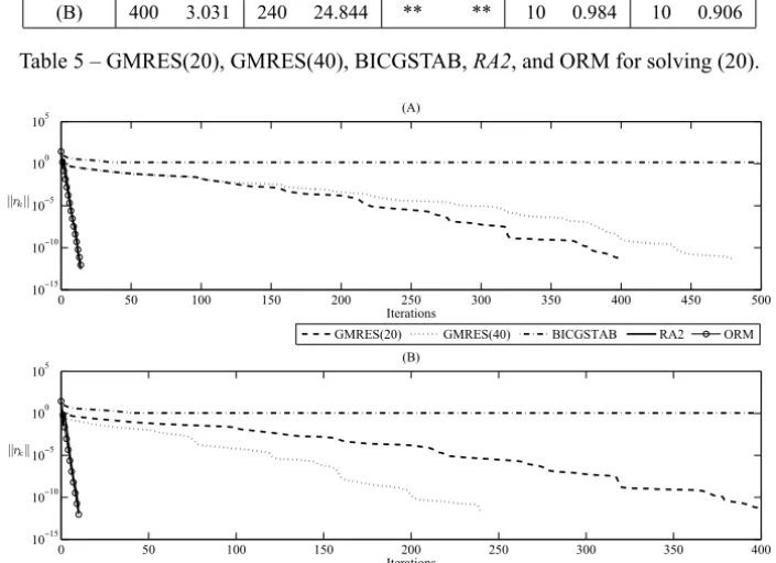
BICGSTAB, ORM, andRA2with the preconditioning strategies (A) and (B). In Table 5 we report the results obtained with GMRES, BICGSTAB, ORM, andRA2 for solving problem (20), when using the preconditioning strategies described in (A) and (B). We setε =10−13 in (18) for stopping the iterations. In Figure 5 we show the behavior of all methods when using preconditioning techniques (A) and (B) for solving (20).
GMRES(20) GMRES(40) BICGSTAB RA2 ORM
Strategy Iter T Iter T Iter T Iter T Iter T
(A) 400 3.297 481 5.094 ** ** 14 0.031 14 0.031 (B) 400 3.031 240 24.844 ** ** 10 0.984 10 0.906
Table 5 – GMRES(20), GMRES(40), BICGSTAB,RA2, and ORM for solving (20).
0 50 100 150 200 250 300 350 400 450 500 1015
1010 105 100 105
Iterations
||rk||
(A)
GMRES(20) GMRES(40) BICGSTAB RA2 ORM
0 50 100 150 200 250 300 350 400 1015
1010 105 100 105
Iterations
||rk||
(B)
Figure 5 – Behavior of all methods when using preconditioning techniques (A) and (B)
for solving (20).
cost and CPU time, without preconditioning. We also observe that RA2 and ORM outperform GMRES and BICGSTAB when preconditioning strategies that reduce the number of cluster of eigenvalues are incorporated.
4 Conclusions
We have compared the performance of the new residual method, as well as the Optimal Richardson Method (ORM), with the restarted GMRES and BICGSTAB, on some test problems, without preconditioning and also using two classical preconditioning strategies (ILU and SSOR). Our preliminary nu-merical results indicate that using the residual direction with a suitable step length can be competitive for solving large-scale problems, and preferable when the eigenvalues are clustered by a preconditioning strategy. Many new precondi-tioning techniques have been recently developed (see e.g., [27, 29] and references therein) that possess the clustering property when dealing with nonsymmetric matrices. In general, any preconditioning strategy that reduces the number of cluster of eigenvalues of the coefficient matrix (suitable for Krylov-subspace methods) should accelerate the convergence of the residual schemes considered in this work. In that sense, theRA2method can be viewed as an extension of the preconditioned residual method, based on the Barzilai-Borwein choice of step length, introduced in [21].
In order to explain the outstanding and perhaps unexpected good behavior of RA2and ORM when an effective preconditioner is applied, it is worth noticing that if the preconditioning matrixC approachesA−1then the steplength chosen byRA2, as well as the one chosen by ORM, approaches 1. Consequently, both preconditioned residual iterations tend to recover Newton’s method for finding the root of the linear mapC Ax−Cb=0, which requires forC = A−1only one iteration to terminate at the solution.
For nonsymmetric systems with an indefinite symmetric part, the proposed general schemeRA1 can not guarantee convergence to solutions of the linear system, and usually convergence to points that satisfy limk→∞rktArk = 0 but
such that limk→∞rk 6=0, as predicted by Theorem 2.1, is observed in practice.
For this type of general linear systems, it would be interesting to analyze in the near future the possible advantages of using ORM with suitable preconditioning strategies.
REFERENCES
[1] O. Axelsson and V.A. Barker,Finite Element Solution of Boundary Value Problems, Theory and Computation. Academic Press, New York (1984).
[2] J. Barzilai and J.M. Borwein.Two-point step size gradient methods. IMA Journal of Numerical Analysis,8(1988), 141–148.
[3] S. Bellavia and B. Morini,A globally convergent newton-gmres subspace method for systems of nonlinear equations. SIAM J. Sci. Comput.,23(2001), 940–960.
[4] E.G. Birgin and J.M. Martínez, A spectral conjugate gradient method for unconstrained optimization. Applied Mathematics and Optimization,43(2001), 117–128.
[5] E.G. Birgin and Y.G. Evtushenko,Automatic differentiation and spectral projected gradient methods for optimal control problems. Optimization Methods and Software,10 (1998), 125–146.
[6] E.G. Birgin, J.M. Martínez and M. Raydan,Nonmonotone spectral projected gradient methods on convex sets. SIAM Journal on Optimization,10(2000), 1196–1211.
[7] C. Brezinski,Variations on Richardson’s method and acceleration. Bull. Soc. Math. Belg., (1996), 33–44.
[8] C. Brezinski,Projection Methods for Systems of Equations. North Holland, Amsterdam (1997).
[9] P. Brown and Y. Saad,Hybrid Krylov methods for nonlinear systems of equations. SIAM J. Sci. Comp.,11(1990), 450–481.
[10] P. Brown and Y. Saad,Convergence theory of nonlinear Newton-Krylov algorithms. SIAM Journal on Optimization,4(1994), 297–330.
[11] D. Calvetti and L. Reichel,Adaptive Richardson iteration based on Leja points. J. Comp. Appl. Math.,71(1996), 267–286.
[12] D. Calvetti and L. Reichel,An adaptive Richardson iteration method for indefinite linear systems. Numer. Algorithms,12(1996), 125–149.
[13] Y.H. Dai and L.Z. Liao,R-linear convergence of the Barzilai and Borwein gradient method. IMA Journal on Numerical Analysis,22(2002), 1–10.
[14] J.E. Jr. Dennis and J.J. Moré,A characterization of superlinear convergence and its appli-cations to quasi-Newton methods. Math. of Comp.,28(1974), 549–560.
[15] M.A. Diniz-Ehrhardt, M.A. Gomes-Ruggiero, J.M. Martínez and S.A. Santos,Augmented Lagrangian algorithms based on the spectral gradient for solving nonlinear programming problems. Journal of Optimization Theory and Applications,123(2004), 497–517. [16] H.C. Elman, D.J. Sylvester and A.J. Wathen,Finite Elements and Fast Iterative Solvers.
[17] R. Fletcher, On the Barzilai-Borwein method. In: Optimization and Control with Applica-tions(L.Qi, K.L. Teo, X.Q. Yang, eds.) Springer, (2005), 235–256.
[18] C.T. Kelley,Iterative Methods for Linear and Nonlinear Equations. SIAM, Philadelphia (1995).
[19] W. La Cruz and M. Raydan, Nonmonotone spectral methods for large-scale nonlinear systems. Optimization Methods and Software,18(2003), 583–599.
[20] W. La Cruz, J.M. Martínez and M. Raydan, Spectral residual method without gradi-ent information for solving large-scale nonlinear systems. Math. of Comp., 75(2006), 1449–1466.
[21] B. Molina and M. Raydan, Preconditioned Barzilai-Borwein method for the numerical solution of partial differential equations. Numerical Algorithms,13(1996), 45–60. [22] M. Raydan,On the Barzilai and Borwein choice of the steplength for the gradient method.
IMA Journal on Numerical Analysis13(1993), 321–326.
[23] M. Raydan,The Barzilai and Borwein gradient method for the large scale unconstrained minimization problem. SIAM Journal on Optimization,7(1997), 26–33.
[24] L. Reichel,The application of Leja points to Richardson iteration and polynomial precon-ditioning. Linear Algebra Appl.,154-156(1991), 389–414.
[25] Y. Saad and M.H. Shultz,GMRES: generalized minimal residual algorithm for solving nonsymmetric linear systems. SIAM J. Sci. Stat. Comput.,7(1986), 856–869.
[26] D.C. Smolarski and P.E. Saylor,An optimum semi-iterative method for solving any linear system with a square matrix. BIT,28(1988), 163–178.
[27] Y. Saad,Iterative Methods for Sparse Linear Systems. SIAM, Philadelphia (2003). [28] H.A. van der Vorst,Bi-CGSTAB: a fast and smoothly convergent variant Bi-CG for the
solution of non-symmetric linear systems. SIAM J. Sci. Stat. Comput.,13(1992), 631–644. [29] H.A. van der Vorst,Iterative Krylov Methods for Large Linear Systems.Cambridge University
Press (2003).
[30] D.M. Young, A historical review of iterative methods. In: A History of Scientific Computing