Influence of aquifer heterogeneity on karst hydraulics and catchment delineation employing distributive modeling approaches

(1)

HESSD

10, 9027–9055, 2013

Influence of aquifer heterogeneity on

karst hydraulics

S. Oehlmann et al.

Title Page

Abstract Introduction

Conclusions References

Tables Figures

◭ ◮

Back Close

Full Screen / Esc

Printer-friendly Version Interactive Discussion

Discussion

P

a

per

|

D

iscussion

P

a

per

|

Discussion

P

a

per

|

Discuss

ion

P

a

per

|

Hydrol. Earth Syst. Sci. Discuss., 10, 9027–9055, 2013 www.hydrol-earth-syst-sci-discuss.net/10/9027/2013/ doi:10.5194/hessd-10-9027-2013

Geoscientiic Geoscientiic

Hydrology and Earth System

Sciences

Open Access

Discussions

This discussion paper is/has been under review for the journal Hydrology and Earth System Sciences (HESS). Please refer to the corresponding final paper in HESS if available.

Influence of aquifer heterogeneity on

karst hydraulics and catchment

delineation employing distributive

modeling approaches

S. Oehlmann1, T. Geyer1, T. Licha1, and S. Birk2

1

Geoscience Center, University of Göttingen, Göttingen, Germany 2

Insitute for Earth Sciences, University of Graz, Graz, Austria

Received: 12 June 2013 – Accepted: 8 July 2013 – Published: 11 July 2013

Correspondence to: S. Oehlmann (sandra.oehlmann@geo.uni-goettingen.de)

(2)

HESSD

10, 9027–9055, 2013

S. Oehlmann et al.

Title Page

Tables Figures

◭ ◮

Back Close

Full Screen / Esc

Discussion

P

a

per

|

D

iscussion

P

a

per

|

Discussion

P

a

per

|

Discuss

ion

P

a

per

|

Abstract

Due to their heterogeneous nature, karst aquifers pose a major challenge for hydroge-ological investigations. Important procedures like the delineation of catchment areas for springs are hindered by the unknown locations and hydraulic properties of highly conductive karstic zones.

5

In this work numerical modeling was employed as a tool in delineating catchment ar-eas of several springs within a karst area in southwestern Germany. For this purpose, different distributive modeling approaches were implemented in the Finite Element sim-ulation software Comsol Multiphysics®. The investigation focuses on the question to which degree the effect of karstification has to be taken into account for accurately

10

simulating the hydraulic head distribution and the observed spring discharges.

The results reveal that the representation of heterogeneities has a large influence on the delineation of the catchment areas. Not only the location of highly conductive elements but also their geometries play a major role for the resulting hydraulic head distribution and thus for catchment area delineation. The size distribution of the karst

15

conduits derived from the numerical models agrees with knowledge from karst genesis. It was thus shown that numerical modeling is a useful tool for catchment delineation in karst aquifers based on results from different field observations.

1 Introduction

Karst aquifers are strongly heterogeneous systems due to a local development of

20

large-scale discontinuities such as conduit systems. This heterogeneity also causes a large anisotropy in the hydraulic parameter field. Conceptually, karst aquifers can be described as dual-flow systems consisting of a fissured matrix with a relatively low hydraulic conductivity and highly conductive karst conduits (Liedl et al., 2003). A characteristic attribute of many karst aquifers is their high discharge focused to large

25

(3)

How-HESSD

10, 9027–9055, 2013

S. Oehlmann et al.

Title Page

Tables Figures

◭ ◮

Back Close

Full Screen / Esc

Discussion

P

a

per

|

D

iscussion

P

a

per

|

Discussion

P

a

per

|

Discuss

ion

P

a

per

|

ever, the delineation of catchment areas of karst springs is still a challenge because of the usually unknown location of large-scale heterogeneities, such as karst conduits, within the aquifer. Common approaches for catchment delineation in porous aquifers like the mapping of geomorphological and topographical features and water balance approaches (Goldscheider and Drew, 2007) are only of limited use in karst systems.

5

Artificial tracer tests provide information about point-to-point connections, but the prac-tical restrictions of tracer investigations prevent using them for completely defining the catchment area. In addition, catchment areas may change under different hydrological conditions, which further complicates the issue.

Numerical groundwater flow simulations are process-based tools that can be used

10

for combining results from di_fferent investigation methods (Geyer et al., 2013) and for augmenting them with physical equations (Birk et al., 2005). There are numerous sim-ulation approaches, which are applicable for karst aquifers. Single continuum models assume the aquifer to be a porous medium that can be divided into representative elementary volumes (REV) (Bachmat and Bear, 1986). The dual flow characteristics

15

of karst aquifers are directly addressed by hybrid or double continuum modeling ap-proaches. Double continuum models simulate groundwater flow in two separate over-lapping continua: a matrix continuum and a conduit continuum, linked via a linear ex-change term (Teutsch, 1989; Mohrlok and Sauter, 1997). Hybrid models include the spatial distribution of local discrete pipe elements representing the major karst conduits

20

coupled to a matrix continuum which represents the properties of the low permeability fissured matrix blocks (Liedl et al., 2003; Birk et al., 2005). Due to the required detailed information and the relatively high numerical e_ffort, the application of hybrid modeling approaches to real karst systems is rare (Reimann et al., 2011a). The highest accuracy regarding the description of aquifer heterogeneities is achieved by discrete multiple

25

(4)

HESSD

10, 9027–9055, 2013

S. Oehlmann et al.

Title Page

Tables Figures

◭ ◮

Back Close

Full Screen / Esc

Discussion

P

a

per

|

D

iscussion

P

a

per

|

Discussion

P

a

per

|

Discuss

ion

P

a

per

|

numerical model is necessary for achieving the aim of the investigation is of primary importance since more complex models require more specific information about the model area and higher numerical effort.

This work analyses how distributive numerical models can be used to support the de-lineation of catchment areas of karst springs. The proposed approach is illustrated

us-5

ing a karst area in southwestern Germany. It is based on the evaluation of the influence of different types of aquifer heterogeneity on the karst flow system. More specifically, the interdependencies between hydraulic head distribution, hydraulic parameters and spring discharges are examined. For this purpose, a homogeneous continuum model and hybrid modeling approaches for flow simulation of a large-scale karst system were

10

set up employing the finite element simulation software Comsol Multiphysics®. These two different modeling approaches were chosen since the geometry of the highly con-ductive conduits was of special interest in this study because of their potential impact on the delineation of the catchment areas. Simulating the conduit geometry with the single continuum approach would have required intense meshing along the karst

con-15

duits needing a very flexible mesh and being numerically highly demanding. Steady state flow equations were implemented for both model types. The three dimensional geometry of the aquifer system was geologically modeled with the software Geological Objects Computer Aided Design®(GoCAD®) and transferred to the Comsol®software.

2 Methods and approach

20

Comsol Multiphysics® is a software that conducts multiphysical simulations using the Finite Element Method (FEM). The different physical properties and equations are stored in di_fferent modules, which can be coupled and adapted as required. The inter-faces used in this work belong to the Subsurface Flow Module, which provides equa-tions for modeling flow in porous media, and to the basic module. All simulaequa-tions were

25

(5)

heterogene-HESSD

10, 9027–9055, 2013

S. Oehlmann et al.

Title Page

Tables Figures

◭ ◮

Back Close

Full Screen / Esc

Discussion

P

a

per

|

D

iscussion

P

a

per

|

Discussion

P

a

per

|

Discuss

ion

P

a

per

|

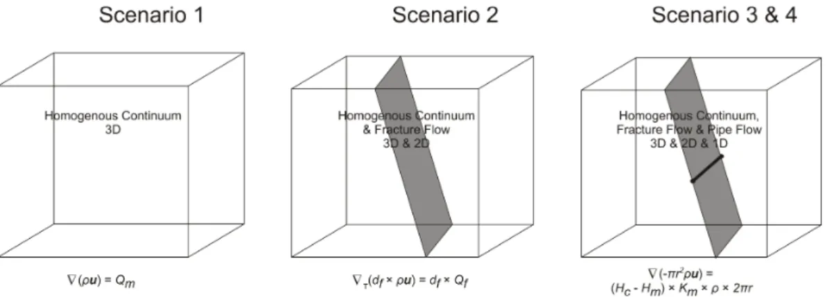
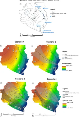
ity several scenarios were set up including more and more characteristic features of karst catchments. Figure 1 schematically shows the simulated scenarios. Catchment areas were derived by importing the simulated water tables from Comsol® to ArcGIS® 10.0 and using the default hydrology tools.

2.1 Scenario 1

5

Scenario 1 simulates a completely homogenous case. It takes into account the thick-ness of the aquifer and boundary conditions given by rivers and surface water divides. Recharge and hydraulic conductivity were kept constant throughout the area. For the flow simulation the Darcy’s Law Interface of the Subsurface Flow Module was used. It calculates the fluid pressure p [M L−1T−2] within the model domain with the Darcy

10

equation (Eq. 1a and 1b).

Qm=∇(ρu) (1a)

u₌₋Km

ρg(∇p+ρg∇D) (1b)

In these equationsQmis the mass source term [M L− 3

T−1],ρis the density of the fluid

15

[M L−3],Km is the hydraulic conductivity of the matrix [L T− 1

] andu_{the Darcy velocity}

[L T−1].gis the magnitude of gravitational acceleration [L T−2] and∇D_{is a unit vector}

in the direction over which the gravity acts. The hydraulic conductivity Km is the only calibration parameter in this scenario.

2.2 Scenario 2

20

(6)

HESSD

10, 9027–9055, 2013

S. Oehlmann et al.

Title Page

Tables Figures

◭ ◮

Back Close

Full Screen / Esc

Discussion

P

a

per

|

D

iscussion

P

a

per

|

Discussion

P

a

per

|

Discuss

ion

P

a

per

|

Groundwater flow in the fracture was simulated with the Fracture Flow Interface of the Subsurface Flow Module implemented in Comsol®. The module requires the definition of the fracture aperturedf [L] and hydraulic conductivity Kf [L T−

1

] inside the fracture. Comsol®assumes that flow processes in the fracture are basically the same as in the surrounding matrix and calculates flow along the fracture with the tangential version

5

of the Darcy equation. The Fracture Flow Module does not allow the application of di_fferent flow laws in the two regions. To simulate two-dimensional fracture flow the term for the fracture aperture is multiplied with both sides of Eq. (1):

df×Qf=∇T(dfρu) (2a)

u₌₋Kf

ρg(∇Tp+ρg∇TD) (2b)

10

withQf being the mass source term for the fracture [M L− 3

T−1] and ∇T the tangential gradient operator. The hydraulic conductivity of the fractureKfis the second calibration parameter beside the matrix conductivityKm(Eq. 1b) in scenario 2.

2.3 Scenario 3

15

In scenario 3, highly conductive conduits were included along the positions of dry val-leys, which are believed to be former riverbeds that have dried up during karstification. For these, 1-D structures are the most fitting representation. Since the Subsurface Flow Module does not offer a similar functionality as Fracture Flow for 1-D elements in 3-D domains, a hybrid model was set up employing Comsol’s PDE Interfaces for simulation

20

of one-dimensional pipes. The interface chosen is called Coefficient Form Edge PDE because it allows calculations along the edges (1-D elements) of a 3-D model. The interface offers a Partial Differential Equation (PDE) (Eq. 3) for which coefficients have to be defined.

f =∇(−c∇v+γ) (3)

(7)

HESSD

10, 9027–9055, 2013

S. Oehlmann et al.

Title Page

Tables Figures

◭ ◮

Back Close

Full Screen / Esc

Discussion

P

a

per

|

D

iscussion

P

a

per

|

Discussion

P

a

per

|

Discuss

ion

P

a

per

|

In Eq. (3),cis defined as the diffusion coefficient,γas the conservative flux source and

f as the source term. By default, the source term is dimensionless. Its unit can be de-fined in the interface and the units of the coefficients are then calculated accordingly.v

is the dependent variable in this equation. In the application using Darcy Flow,v corre-sponds to the pressurep[M L−1T−2]. The source termf equals the mass source term

5

Qmof the Darcy equation (Eq. 1a). The first of the remaining terms describes the effect of water pressure gradients, the other one the effect of gravitation (compare Eq. 1b). In this case the diffusion coefficient c depends on the hydraulic conduit conductivity

Kc, which is normalized for a unit cross sectional area. Thus, after multiplying with the conduit areaπr2Eq. (3) translates to Eq. (4). The conduit area term replaces the two

10

missing dimensions while performing simulations in 1-D elements in a 3-D domain.

πr2×Qm=∇

−πr2Kc

g ∇p−πr

2_ρK

c∇D

(4)

The source term multiplied with the conduit area πr2×Q_m is equal to the mass exchange of water per unit length between the matrix and the conduit [M L−1T−1]. Reimann et al. (2011b) define the exchange term between a karst conduit and the

15

rock matrix as:

qex=

K′

b′ ×Pex∆hex. (5)

q_ex is the exchange flow per unit length [L2T−1], ∆h_ex is the difference between the hydraulic head in the matrix and the hydraulic head in the conduit [L],Pexthe exchange perimeter [L] andK′/b′ the leakage coefficient [T−1]. For this simulation the equation

20

was simplified by assuming the exchange perimeter equal to the pipe perimeter. As-suming there is no barrier between the conduit and the matrix the leakage coefficient is equal to the hydraulic conductivity of the matrix divided by the theoretical distanceL[L] over which the hydraulic head difference is calculated.Lis kept at unit length through-out the simulation. The equation of Reimann et al. (2011b) is multiplied by the density

(8)

HESSD

10, 9027–9055, 2013

S. Oehlmann et al.

Title Page

Tables Figures

◭ ◮

Back Close

Full Screen / Esc

Discussion

P

a

per

|

D

iscussion

P

a

per

|

Discussion

P

a

per

|

Discuss

ion

P

a

per

|

for obtaining the mass exchange term. The resulting exchange equation is defined in Eq. (6):

πr2×Qm=(Hc−Hm)×

Km

L ×ρ×2πr (6)

withHcbeing the hydraulic head in the conduit andHmbeing the hydraulic head in the matrix [L]. 2πr is the perimeter of the pipe [L]. The exchange term is used as mass

5

flux for the matrix and as mass source for the conduits with a changed algebraic sign. Dirichlet conditions were set as boundary conditions at the springs.

2.4 Scenario 4

Scenario 4 was based on the same structure of the conduit system as scenario 3 but differed in the assumption for the conduit radius. While for scenario 3 the radius is

10

constant within the entire conduit system, for scenario 4 a change in conduit radius towards the spring was introduced. Liedl et al. (2003) showed with their karst genesis simulations that for a conduit derived from solution processes a change in diameter is likely to occur along its extent. They introduced several simulations with different boundary conditions and derived di_fferent types of solutional widening and resulting

15

conduit shapes.

For situations where diffuse recharge prevails, Liedl et al. (2003) showed a nearly linear increase in conduit diameters towards a karst spring. Thus, in scenario 4 a linear widening function was applied to each conduit along its arc length. At each intersection the radii of both branches were added to account for the larger volume of water flowing

20

there. The largest simulated radius is 4.6 m at the main karst spring.

3 Field site

(9)

HESSD

10, 9027–9055, 2013

S. Oehlmann et al.

Title Page

Tables Figures

◭ ◮

Back Close

Full Screen / Esc

Discussion

P

a

per

|

D

iscussion

P

a

per

|

Discussion

P

a

per

|

Discuss

ion

P

a

per

|

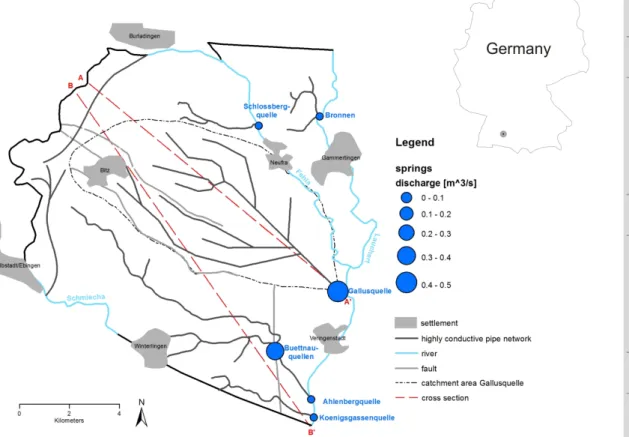
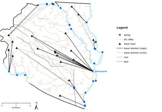
located within the investigation area of approximately 150 km2 (Fig. 3). The size of its catchment area is estimated to be 45 km2based on a water balance approach and artificial tracer tests (Sauter, 1992) (Fig. 3). The spring is used for drinking water supply of approximately 40 000 people and has an average annual discharge of 0.5 m3s−1. It is a suitable location for distributive karst modeling due to the extensive studies that have

5

been conducted in the area before (e.g. Sauter, 1992; Geyer et al., 2007; Hillebrand et al., 2012).

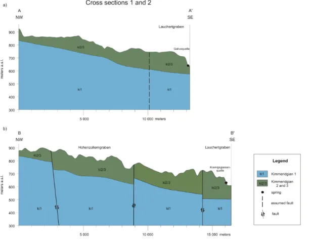
Geologically the area consists of Upper Jurassic limestone and marlstone. The main aquifer is composed primarily of massive and layered limestone of the Kimmeridgian 2 and 3 (ki2/3). Beneath those rocks there are marly limestones and marlstones of

10

the Kimmeridgian 1 (ki1) which mainly act as aquitards due to their lower solubility. Two major fault zones cross the model area. The Hohenzollerngraben strikes north-west to southeast, the Lauchertgraben crosses the area in the East striking north to south (Fig. 2). While there is no information about the hydraulic conductivity of the Lauchertgraben fault zones, the Hohenzollerngraben was crossed by tunneling

15

work related to the construction of a regional water pipeline (Albstollen, Bodensee-Wasserversorgung). The northern boundary fault was found to be highly conductive from the significant amount of water entering the tunnel while crossing it (Gwinner et al., 1993). A high hydraulic conductivity of this zone can further be assumed from the fact that the Gallusquelle spring lies exactly at the extension of this fault where it

20

meets the river Lauchert (Fig. 2).

4 Model design and calibration

The model area is constrained by fixed head boundaries at the rivers Lauchert, Fehla and Schmiecha (Dirichlet boundaries). No flow boundaries are derived from the dip of the aquifer base and artificial tracer test information (Fig. 3). The size of the model

25

(10)

af-HESSD

10, 9027–9055, 2013

S. Oehlmann et al.

Title Page

Tables Figures

◭ ◮

Back Close

Full Screen / Esc

Discussion

P

a

per

|

D

iscussion

P

a

per

|

Discussion

P

a

per

|

Discuss

ion

P

a

per

|

ter Gwinner et al. (1993). Highly conductive pipes connected to the Gallusquelle spring were implemented according to Mohrlok and Sauter (1997) and Doummar et al. (2012). The lateral positions of model boundaries, highly conductive faults and the pipe network along dry valleys were constructed in ArcGIS®10.0 and imported to Comsol®as 2-D dxf-files or interpolation curves. Vertically, the highly conductive conduits were

posi-5

tioned approximately at the elevation of the water table simulated in scenario 1. The highly conductive 2-D fracture for scenario 2 was positioned along the northern fault of the Hohenzollerngraben. The documented fault was linearly extended to the East to cross the river Lauchert at the position of the Gallusquelle spring (compare Fig. 5a and c).

10

Vertically the model consists of two layers. The upper one represents the aquifer. In the East it stretches from ground surface to the base of the Kimmeridgian 2 (ki2). The formation is tapering out in the West of the area but reaches a thickness of over 200 m in the East where the Gallusquelle spring is located. In the West the underlying Kimmeridgian 1 (ki1) approaches the surface until it crops out. In that region it shows

15

karstification and thus is part of the aquifer. The depth of the karstification was derived from drilling cores. The unkarstified ki1 acts as aquitard and composes the second vertical layer of the model. It was simulated down to a horizontal depth of 300 m a.s.l. since its lower boundary is not expected to influence the simulation. The ground surface is defined by a Digital Elevation Model (DEM) with a cell size of 40 m. The position of

20

the ki2 base was derived from boreholes and a base map provided in Sauter (1992). Two cross sections were constructed through the model area for illustrating the geology (Fig. 4). Their positions are illustrated in Fig. 2.

Current Comsol® software has major difficulties interpolating irregular surfaces that cannot be described by analytical functions. Therefore, the three-dimensional position

25

(11)

HESSD

10, 9027–9055, 2013

S. Oehlmann et al.

Title Page

Tables Figures

◭ ◮

Back Close

Full Screen / Esc

Discussion

P

a

per

|

D

iscussion

P

a

per

|

Discussion

P

a

per

|

Discuss

ion

P

a

per

|

3-D domains. At the ground surface a constant recharge was applied as a Neumann condition. The base of the model was defined as a no flow boundary, while the base of the aquifer was set as a continuity boundary allowing undisturbed water transfer. The exact values for all model parameters are provided in Table 1.

The model was calibrated employing Comsol Multiphysics® Parametric Sweep

op-5

tion, which calculates several model runs considering di_fferent parameter combina-tions. The focus of the calibration lay on the hydraulic head distribution. The measured hydraulic head values are long-term averages derived from twenty measuring stations that are distributed within the model area.

For the calibration of spring discharges five smaller springs were included in the

10

model besides the Gallusquelle spring. Other springs within the investigation area are either very small or have not been measured on a regular basis for reliably estimating their average annual discharges. The Gallusquelle spring and three of the other springs considered in the model calibration, the Bronnen spring, the Ahlenbergquelle spring and the Königsgassenquelle spring, are located at the river Lauchert; the

Schloss-15

bergquelle spring is situated at the river Fehla; a group of springs called the Büt-tnauquellen springs is located at a dry valley (Gwinner et al., 1993; Golwer et al., 1978) (Fig. 2). The Büttnauquellen springs and the Ahlenbergquelle spring probably share most of their catchment area and are likely to be fed by the same karst con-duit network (Fig. 2). Localized discharge was also simulated into the rivers Fehla and

20

Schmiecha in the West of the area, where several springs exist (Fig. 3). The highly con-ductive karst conduits used in the simulation connect points in the proximity of the Ho-henzollerngraben with the Fehla-Ursprung spring at the Fehla and the Balinger Quelle spring at the Schmiecha. The karst conduits were identified by tracer tests (Fig. 3). However, there is not enough data for the discharges of the Fehla-Ursprung spring and

25

(12)

HESSD

10, 9027–9055, 2013

S. Oehlmann et al.

Title Page

Tables Figures

◭ ◮

Back Close

Full Screen / Esc

Discussion

P

a

per

|

D

iscussion

P

a

per

|

Discussion

P

a

per

|

Discuss

ion

P

a

per

|

within a range of 10 L s−1, if this could be achieved with a reasonable fit for the hydraulic head distribution.

The radii of the highly conductive conduits were calibrated for a conduit volume of 200 000 m3 for the Gallusquelle catchment that was deduced from an artificial tracer test (Geyer et al., 2008). For the other springs in the model area, there was no such

5

information. For scenario 3 a systematic approach for relating the cross-sectional ar-eas of the conduits connected to each spring to the one of the Gallusquelle spring was employed. The conduit area for each spring was defined as the area for the Gal-lusquelle spring multiplied by the ratio of the spring discharge to the discharge of the Gallusquelle spring. For scenario 4 where a linear relationship between the arc length

10

and the conduit diameter was defined, it was assumed that the shorter conduits of the smaller springs lead to accordingly smaller cross-sectional areas without any further adjustments. At the springs, fixed head boundary conditions were set at the conduits.

5 Results and discussion

The four scenarios were evaluated and compared regarding hydraulic head distribution,

15

hydraulic parameters, spring discharges and catchment area delineations. Figure 5 shows the simulated hydraulic head distributions for all scenarios. They are compared to a hydraulic head contour map that Sauter (1992) constructed based on field mea-surements (Fig. 5a). The calibration parameters can be found in Table 1. Table 2 and Fig. 6 compare the simulated and observed spring discharges.

20

5.1 Hydraulic head distribution

The model can approximate the hydraulic head distribution in all scenarios. However, there is a significant difference of the model fit between scenario 1 with a Root Mean Square Error (RMSE) of 15 m and the best fit (scenario 4) with a RMSE of 7.7 m. Sce-nario 2 and 3 show similar RMSE of about 13 m. The measured hydraulic heads show

(13)

HESSD

10, 9027–9055, 2013

S. Oehlmann et al.

Title Page

Tables Figures

◭ ◮

Back Close

Full Screen / Esc

Discussion

P

a

per

|

D

iscussion

P

a

per

|

Discussion

P

a

per

|

Discuss

ion

P

a

per

|

a lateral change in hydraulic gradients. In accordance with observations in the karst aquifer of Mammoth Cave (Kentucky, USA) reported by Worthington (2009), the Gal-lusquelle catchment shows lower hydraulic gradients in the East towards the spring than in the rest of the area. This is probably caused by the higher hydraulic conduc-tivity due to the higher karstification in the vicinity of the karst spring. After

Worthing-5

ton (2009) this is one of the typical characteristics of karst areas. The observation is also supported by Liedl et al. (2003) who found a widening of karst conduits in spring direction. At the field site, the steepest hydraulic head gradients were observed in the central area.

Scenario 1 cannot reproduce this behavior of the hydraulic gradient. It shows the

10

opposite of the observed gradient distribution with steeper gradients close to the river Lauchert, where most of the springs are located. This e_ffect usually occurs in homoge-neous aquifers with evenly distributed recharge conditions. The highly conductive frac-ture in scenario 2 crosses the model area completely from West to East. Therefore, it mainly lowers the hydraulic head values in the central and western part, thus opposing

15

the observed gradient distribution. In the West, where the fault starts to drain the area, its very high transmissivity leads to a strong distortion of hydraulic head contour lines.

The conduit network in Scenario 3 drains the area predominantly in the central part. This results in a much lower hydraulic gradient than actually observed in the field (Fig. 5d). This effect is due to the constant and relatively high conduit

diame-20

ter of 2.56 m for the conduits connected to the Gallusquelle spring. This allows large amounts of water to flow into the conduits in the central part of the catchment. While the low hydraulic conductivity of the matrix is limiting groundwater flow in this part of the catchment, the ability of the conduits to conduct water becomes limiting close to the Gallusquelle spring and causes water to flow out of the conduits and back into the

25

matrix. According to the classification after Kovács et al. (2005) the flow regime in this part of the model area thus is conduit-influenced.

(14)

kars-HESSD

10, 9027–9055, 2013

S. Oehlmann et al.

Title Page

Tables Figures

◭ ◮

Back Close

Full Screen / Esc

Discussion

P

a

per

|

D

iscussion

P

a

per

|

Discussion

P

a

per

|

Discuss

ion

P

a

per

|

tification and thus higher transmissivity close to the spring. As a consequence, the hydraulic gradient is steeper in the central part of the catchment than close to the spring (Fig. 5e). This corresponds to the matrix-influenced flow regime according to Kovács et al. (2005), where the discharge is controlled by the matrix rather than by the conduits. The effect is not strong enough to completely avoid an overestimation of

5

hydraulic heads in the East and an underestimation in the central part and in the West. This leads to the assumption that the change in gradient is not purely derived from the higher karstification but that other, probably geologic factors contribute to the lat-eral differences in hydraulic conductivity. A more dendritic and farther extended conduit system could also lower the hydraulic head in the East. Due to the gradual widening

10

of the conduits, the troughs in the hydraulic head contour lines are less pronounced in scenario 4 than in scenario 3 and occur further east.

5.2 Hydraulic parameters

Between the scenarios, a trend for the matrix conductivity K_m can be observed. The highest value is obtained in scenario 1 with 5.1×10−5m s−1. This is due to the fact

15

that Km for the homogeneous case averages the hydraulic conductivities of all struc-tures in the area, since none of the discrete feastruc-tures is considered individually. The highly conductive fracture in scenario 2 allows for faster water transport and therefore lower hydraulic heads can be achieved with a lower value for the matrix conductiv-ity of 3.1×10−5m s−1. This trend continues for scenario 3 and 4, where Km drops to

20

2.3×10−5m s−1and 2.6×10−5m s−1, respectively.

The fracture conductivity Kf is introduced in scenario 2. Despite being in the typ-ical range of literature of 3–10 m s−1 (Sauter, 1992) the obtained value of 2.7 m s−1 probably is too low, because all other karst features, which can drain water from the Gallusquelle catchment towards other springs, are neglected. If additional highly

con-25

(15)

HESSD

10, 9027–9055, 2013

S. Oehlmann et al.

Title Page

Tables Figures

◭ ◮

Back Close

Full Screen / Esc

Discussion

P

a

per

|

D

iscussion

P

a

per

|

Discussion

P

a

per

|

Discuss

ion

P

a

per

|

for the relatively high conduit conductivity Kc of 6.5 m s− 1

in scenario 3. Even though the discharge at the Gallusquelle spring is the same as well as the integrated conduit volume, the conduit conductivity of 2 m s−1obtained for scenario 4 is significantly lower than the value of 6.5 m s−1 obtained for scenario 3. This is because the karst conduit system with constant diameter needs a higher overall transmissivity to transport the

5

same amount of water due to limiting flow capacity of the conduits close to the spring. The conduit diameter in scenario 3 corresponds to a representative constant diame-ter for the Gallusquelle spring. Birk et al. (2005) used artificial tracer tests for calculating the representative diameter. The authors calculated a diameter of about 5 m, which is higher than the 2.56 m simulated with scenario 3. This is probably due to the fact that

10

these tracer tests were conducted approximately 3 km northwest of the spring while in the model the conduits extend approximately 10 km to the Northwest. Thus, this sup-ports the idea that the diameters of the conduits closer to the spring are higher than those farther away (see Sect. 2.4).

5.3 Spring discharge

15

Scenario 1 fails to simulate the locally increased discharge at the karst springs (Ta-ble 2). Since there are no areas of focused flow, there is only diffuse groundwater dis-charge into the rivers, mainly the Lauchert. In scenario 2 fracture flow along the fault allows the simulation of increased discharge at the Gallusquelle spring (Table 2). The other springs that were not connected to highly conductive elements show no locally

20

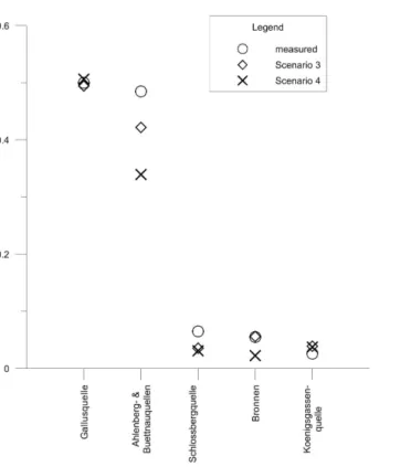
increased discharge (Table 2). The slightly raised discharge of the Schlossbergquelle spring compared to scenario 1 results from generally increased water flow into the river Fehla, not from locally raised discharge at the spring location. The local discharges at all springs can only be represented by scenarios 3 and 4. The simulation is satisfac-tory for both scenarios. The simulated discharge of the scenarios is very similar for the

25

(16)

dis-HESSD

10, 9027–9055, 2013

S. Oehlmann et al.

Title Page

Tables Figures

◭ ◮

Back Close

Full Screen / Esc

Discussion

P

a

per

|

D

iscussion

P

a

per

|

Discussion

P

a

per

|

Discuss

ion

P

a

per

|

charge is slightly overestimated for the Königsgassenquelle spring and underestimated for the Schlossbergquelle spring. Since the Schlossbergquelle spring is the only spring included at the river Fehla and no registration of discharge values of the river itself was conducted, it cannot be distinguished, if the underestimation at the Schlossbergquelle spring is due to an inexact karst conduit network or to an underestimated discharge

5

into the river. For the Bronnen spring, different results can be observed for the two sce-narios. While scenario 3 has a very good fit, scenario 4 underestimates the discharge. This suggests that the conduits leading to the spring are assumed too short in the simulation leading to underestimated conduit diameters in scenario 4.

The most pronounced difference between the two simulations occurs at the

Büt-10

tnauquellen and Ahlenbergquelle springs. Both simulations underestimate their dis-charge with a significantly stronger underestimation in scenario 4 (Fig. 6). This is probably due to the simplified approach of treating them like a single spring and at-taching them to the same conduit. While the Ahlenbergquelle spring is perennial, the Büttnauquellen springs are intermittent. This suggests that there are karst conduits in

15

at least two different depths and thus that the representation with a conduit network in a single depth is not adequate. A too short conduit system with too little side branches has a stronger impact on scenario 4 because of the dependence of diameters on the total length and amount of intersections leading to a stronger underestimation of con-duit volumes than in scenario 3.

20

5.4 Catchment area delineation

The spring catchment areas were delineated according to the hydraulic heads within the matrix. For the delineation a bending of contour lines towards the springs is re-quired, meaning they can only be generated with localized discharge at the spring positions. Therefore no catchment areas can be delineated in scenario 1. In scenario

25

(17)

hy-HESSD

10, 9027–9055, 2013

S. Oehlmann et al.

Title Page

Tables Figures

◭ ◮

Back Close

Full Screen / Esc

Discussion

P

a

per

|

D

iscussion

P

a

per

|

Discussion

P

a

per

|

Discuss

ion

P

a

per

|

draulic conductivity of the fault is assumed to be constant, it receives most of the inflow in the West and cannot receive more water close to the spring. Thus, the catchment area mainly includes the western part of the model area (Fig. 5c).

In scenario 3 catchment areas can be simulated for the Gallusquelle spring and for the Büttnauquellen and Ahlenbergquelle springs (Fig. 5d). The strange looking shape

5

of the areas is caused by the early filling of the conduits with water in the West of the model domain which prevents drainage of the fissured matrix by the conduit system in the East of the area. Therefore the Gallusquelle spring mainly receives water from the western part of the area, where its conduits drain enormous water volumes due to their relatively large diameter. Due to outflow of water into the matrix in the East,

10

only part of the water from the shown catchment area is transported to the springs. In the West it can be observed that the catchment areas of the Gallusquelle spring and the Büttnauquellen and Ahlenbergquelle springs reach across karst conduits leading to other springs (Fig. 5d). In this case the catchment areas of the springs overlap. The catchment areas were constructed in 2-D according to surface values, so that

15

they envision the flow above the smaller conduits in the West. In the East it can be observed that the catchment areas do not include all parts of the respective karst conduit network. In these areas the conduits cannot accommodate more water and outflow occurs. The catchment area for the Gallusquelle spring that was delineated in scenario 3 includes all but one tracer test conducted. The Gallusquelle spring drains

20

nearly all water from the springs at the river Fehla. The hydraulic heads in the West are lowered leading to influent flow conditions along parts of the western Fehla. This contradicts the development of several springs in this area and makes this scenario highly unlikely (compare Fig. 3).

Scenario 4 is the only simulation leading to reasonable results regarding the

catch-25

(18)

under-HESSD

10, 9027–9055, 2013

S. Oehlmann et al.

Title Page

Tables Figures

◭ ◮

Back Close

Full Screen / Esc

Discussion

P

a

per

|

D

iscussion

P

a

per

|

Discussion

P

a

per

|

Discuss

ion

P

a

per

|

estimation of spring discharge (Table 2). Since the underestimation is more pronounced for scenario 4 than for scenario 3, the catchment area is significantly smaller (compare Fig. 5d and c). A small overlap of catchment areas can still be observed in the West but in scenario 4 the Gallusquelle only drains small amounts of water from the western part, so that the western Fehla is completely effluent.

5

For the smaller springs, no catchment areas could be generated in either of the scenarios. They produce a very small ratio of the total discharge of the model area (<5 %) and the resolution of the simulation was not fine enough to reliably draw their catchment boundaries.

6 Conclusions

10

The results show that distributive numerical simulation is a useful tool for approach-ing the complex subject of subsurface catchment delineation in karst aquifers as long as effects of karstification are sufficiently taken into account. Even though the Gal-lusquelle area is significantly less karstified than for example the Mammoth Cave (Ken-tucky, USA) (Worthington, 2009) and does not show significant troughs in the hydraulic

15

head contour lines, it cannot be simulated with a homogeneous hydraulic parameter field. The geometry of the conduits is of major importance for the simulation. Although the Gallusquelle spring is positioned on the linear extension of the northern fault of the Hohenzollerngraben the hydraulic conditions cannot correctly be simulated without consideration of dry valleys. For catchment delineation, the approach of using conduits

20

with constant geometric parameters is not satisfactory, either. While it is possible to fit spring discharges with a double continuum model (e.g. Kordilla et al., 2012) or a sin-gle continuum model with a highly conductive zone with constant hydraulic properties (e.g. Doummar et al., 2012) the hydraulic head distribution and hydraulic conductivities cannot be correctly approximated with these approaches.

25

(19)

HESSD

10, 9027–9055, 2013

S. Oehlmann et al.

Title Page

Tables Figures

◭ ◮

Back Close

Full Screen / Esc

Discussion

P

a

per

|

D

iscussion

P

a

per

|

Discussion

P

a

per

|

Discuss

ion

P

a

per

|

head distribution and the spring discharges were found to be strongly dependent on the selected geometry of the highly conductive elements it seems unavoidable to bet-ter constrain their positions and sizes in the area. In case of the Gallusquelle area the smooth hydraulic gradients do not allow the localization of conduits by troughs in the hy-draulic head contour lines like in some other karst areas (e.g. Joodi et al., 2010). Karst

5

genesis simulation would provide process-based information about conduit widening towards a karst spring. Such a simulation would be possible to conduct with Comsol Multiphysics®, given sufficient input data.

Acknowledgements. The presented study was funded by the German Federal Ministry of

Ed-ucation and Research (promotional reference No. 02WRS1277A, AGRO, “Risikomanagement 10

von Spurenstoffen und Krankheitserregern in ländlichen Karsteinzugsgebieten”) and by the Austrian Science Fund (FWF): L576-N21. Tracer test data was provided by the Landesamt für Geologie, Rohstoffe und Bergbau (LGRB).

This Open Access Publication is funded by the University of Göttingen. 15

References

Bachmat, Y. and Bear, J.: Macroscopic modelling of transport phenomena in porous media, 1: The continuum approach, Transport Porous Med., 1, 213–240, 1986.

Birk, S., Geyer, T., Liedl, R., and Sauter, M.: Process-based interpretation of tracer tests in carbonate aquifers, Ground Water, 43, 381–388, 2005.

20

Doummar, J., Sauter, M., and Geyer, T.: Simulation of flow processes in a large scale karst sys-tem with an integrated catchment model (Mike She) – identification of relevant parameters in-fluencing spring discharge, J. Hydrol., 426–427, 112–123, doi:10.1016/j.jhydrol.2012.01.021, 2012.

Geyer, T., Birk, S., Licha, T., Liedl, R., and Sauter, M.: Multi-tracer test approach to characterize 25

reactive transport in karst aquifers, Ground Water, 45, 36–45, 2007.

(20)

HESSD

10, 9027–9055, 2013

S. Oehlmann et al.

Title Page

Tables Figures

◭ ◮

Back Close

Full Screen / Esc

Discussion

P

a

per

|

D

iscussion

P

a

per

|

Discussion

P

a

per

|

Discuss

ion

P

a

per

|

Geyer, T., Birk, S., Reimann, T., Dörfliger, N., and Sauter, M.: Differentiated characterization of karst aquifers: some contributions, Carbonate. Evaporite., 28, 41–46, doi:10.1007/s13146-013-0150-9, 2013.

Goldscheider, N. and Drew, D.: Combined use of methods, in: Methods in Karst Hydrogeology, International contributions to hydrogeology, 26, Taylor & Francis, London, 223–228, 2007. 5

Golwer, A., Koerner, U., Villinger, E., and Werner, J.: Erläuterungen zu Blatt 7821 Veringenstadt, Geologische Karte 1 : 25 000 von Württemberg, Geologisches Landesamt Baden-Württemberg, Stuttgart, 151 pp., 1978.

Gwinner, M. P., Villinger, E., and Schreiner, A.: Erläuterungen zu Blatt 7721 Gammertingen, Geologische Karte 1 : 25 000 von Württemberg, Geologogisches Landesamt Baden-10

Württemberg, Freiburg/Stuttgart, 78 pp., 1993.

Hillebrand, O., Nödler, K., Licha, T., Sauter, M., and Geyer, T.: Identification of the attenuation potential of a karst aquifer by an artificial dualtracer experiment with ca_ffeine, Water Res., 46, 5381–5388, 2012.

Joodi, A. S., Sizaret, S., Binet, S., Bruand, A., Alberic, P., and Lepiller, M.: Development of 15

a Darcy-Brinkman model to simulate water flow and tracer transport in a heterogenous karstic aquifer (Val d’Orléans, France), Hydrogeol. J., 18, 295–309, doi:10.1007/s10040-009-0536-x, 2010.

Kordilla, J., Sauter, M., Reimann, T., and Geyer, T.: Simulation of saturated and unsaturated flow in karst systems at catchment scale using a double continuum approach, Hydrol. Earth 20

Syst. Sci., 16, 3909–3923, doi:10.5194/hess-16-3909-2012, 2012.

Kovács, A., Perrocket, P., Király, L., and Jeannin, P. Y.: A quantitative method for the charac-terisation of karst aquifers based on spring hydrograph analysis, J. Hydrol., 303, 152–164, 2005.

Liedl, R., Sauter, M., Hückinghaus, D., Clemens, T., and Teutsch, G.: Simulation of the devel-25

opment of karst aquifers using a coupled continuum pipe flow model, Water Resour. Res., 39, 1057, doi:10.1029/2001WR001206, 2003.

Mohrlok, U. and Sauter, M.: Modelling groundwater flow in a karst terraine using discrete and double-continuum approaches: importance of spatial and temporal distribution of recharge, in: Proceedings of the 12th International Congress of Speology, 2/6th Conference on Lime-30

(21)

HESSD

10, 9027–9055, 2013

S. Oehlmann et al.

Title Page

Tables Figures

◭ ◮

Back Close

Full Screen / Esc

Discussion

P

a

per

|

D

iscussion

P

a

per

|

Discussion

P

a

per

|

Discuss

ion

P

a

per

|

Reimann, T., Rehrl, C., Shoemaker, W. B., Geyer, T., and Birk, S.: The significance of tur-bulent flow representation in single-continuum models, Water Resour. Res., 47, W09503, doi:10.1029/2010WR010133, 2011a.

Reimann, T., Geyer, T., Shoemaker, W. B., Liedl, R., and Sauter, M.: Effects of dynamically variable saturation and matrix-conduit coupling of flow in karst aquifers, Water Resour. Res., 5

47, W11503, doi:10.1029/2011WR010446, 2011b.

Sauter, M.: Quantification and Forecasting of Regional Groundwater Flow and Transport in a Karst Aquifer (Gallusquelle, Malm, SW Germany), Tübinger Geowissenschaftliche Ar-beiten, C13, Tübingen, 1992.

Teutsch, G.: Groundwater models in karstified terrains: two practical examples from the 10

Swabian Alb (S. Germany), in: Proceedings of the 4th Conference – Solving Groundwater Problems with Models, 7–9 February 1989, Indianapolis, USA, 11 pp., 1989.

Teutsch, G. and Sauter, M.: Groundwater modeling in karst terranes: scale e_ffects, data aqui-sition and field validation, in: Proceedings of the 3rd Conference on Hydrogeology, Ecol-ogy, Monitoring and Management of Ground Water in Karst Terranes, 4–6 December 1991, 15

Nashville, USA, 17–34, 1991.

(22)

HESSD

10, 9027–9055, 2013

S. Oehlmann et al.

Title Page

Tables Figures

◭ ◮

Back Close

Full Screen / Esc

Discussion

P

a

per

|

D

iscussion

P

a

per

|

Discussion

P

a

per

|

Discuss

ion

P

a

per

|

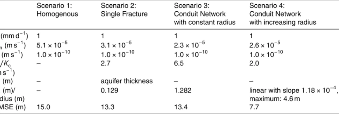
Table 1.Input and calibration values of the different scenarios. The root mean square error of

the hydraulic head distribution is given as an index for the quality of the model fit.

Scenario 1: Homogenous

Scenario 2: Single Fracture

Scenario 3: Conduit Network with constant radius

Scenario 4: Conduit Network with increasing radius

R(mm d−1) 1 1 1 1

Km(m s− 1

) 5.1×10−5 3.1×10−5 2.3×10−5 2.6×10−5

Kl(m s−1) 1.0×10−10 1.0×10−10 1.0×10−10 1.0×10−10 Kf/Kc

(m s−1)

– 2.7 6.5 2.0

dz(m) – aquifer thickness – –

dy(m)/

radius (m)

– 0.129 1.282 linear with slope 1.18_×10−4, maximum: 4.6 m

RMSE (m) 15.0 13.3 13.4 7.7

R=groundwater recharge by precipitation,Km=hydraulic conductivity of matrix,Kl=hydraulic conductivity of lowly conductive ki1,Kf=hydraulic conductivity of fracture,Kc=hydraulic conductivity of conduits,dz=fracture depth,dy=fracture aperture, RMSE=root mean square error for the

(23)

HESSD

10, 9027–9055, 2013

S. Oehlmann et al.

Title Page

Tables Figures

◭ ◮

Back Close

Full Screen / Esc

Discussion

P

a

per

|

D

iscussion

P

a

per

|

Discussion

P

a

per

|

Discuss

ion

P

a

per

|

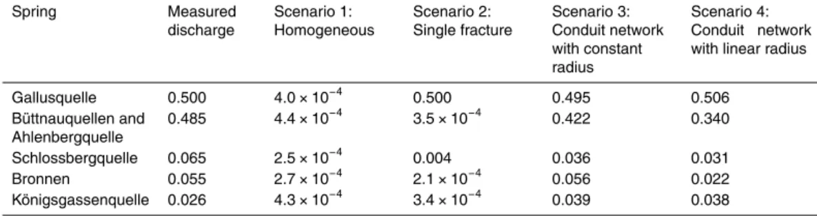
Table 2.Simulated spring discharges (m3s−1) for all scenarios.

Spring Measured discharge

Scenario 1: Homogeneous

Scenario 2: Single fracture

Scenario 3: Conduit network with constant radius

Scenario 4: Conduit network with linear radius

Gallusquelle 0.500 4.0×10−4 0.500 0.495 0.506 Büttnauquellen and

Ahlenbergquelle

0.485 4.4×10−4 _3.5

×10−4 _0.422 _0.340

(24)

HESSD

10, 9027–9055, 2013

S. Oehlmann et al.

Title Page

Tables Figures

◭ ◮

Back Close

Full Screen / Esc

Discussion

P

a

per

|

D

iscussion

P

a

per

|

Discussion

P

a

per

|

Discuss

ion

P

a

per

|

Fig. 1.Conceptual geometry of the simulated scenarios. For explanation of the flow equations

(25)

HESSD

10, 9027–9055, 2013

S. Oehlmann et al.

Title Page

Tables Figures

◭ ◮

Back Close

Full Screen / Esc

Discussion

P

a

per

|

D

iscussion

P

a

per

|

Discussion

P

a

per

|

Discuss

ion

P

a

per

|

Fig. 2.Model area, including the catchment of the Gallusquelle spring and positions of all

(26)

HESSD

10, 9027–9055, 2013

S. Oehlmann et al.

Title Page

Tables Figures

◭ ◮

Back Close

Full Screen / Esc

Discussion

P

a

per

|

D

iscussion

P

a

per

|

Discussion

P

a

per

|

Discuss

ion

P

a

per

|

Fig. 3.Top view of the model area. Tracer tests within the area are illustrated with their major

(27)

HESSD

10, 9027–9055, 2013

S. Oehlmann et al.

Title Page

Tables Figures

◭ ◮

Back Close

Full Screen / Esc

Discussion

P

a

per

|

D

iscussion

P

a

per

|

Discussion

P

a

per

|

Discuss

ion

P

a

per

|

Fig. 4.Cross sections of the study area as constructed in GoCAD®from northwest to southeast

(28)

HESSD

10, 9027–9055, 2013

S. Oehlmann et al.

Title Page

Tables Figures

◭ ◮

Back Close

Full Screen / Esc

Discussion

P

a

per

|

D

iscussion

P

a

per

|

Discussion

P

a

per

|

Discuss

ion

P

a

per

|

Fig. 5.Hydraulic head distributions and simulated catchment areas.(a) After Sauter (1992),

(29)

HESSD

10, 9027–9055, 2013

S. Oehlmann et al.

Title Page

Tables Figures

◭ ◮

Back Close

Full Screen / Esc

Discussion

P

a

per

|

D

iscussion

P

a

per

|

Discussion

P

a

per

|

Discuss

ion

P

a

per

|

Fig. 6.Spring discharge: measured and simulated values using a conduit network with constant