ISSN 0104-6632 Printed in Brazil
www.abeq.org.br/bjche
Vol. 26, No. 01, pp. 207 - 218, January - March, 2009
Brazilian Journal
of Chemical
Engineering
EXPERIMENTAL PURIFICATION OF PACLITAXEL
FROM A COMPLEX MIXTURE OF TAXANES
USING A SIMULATED MOVING BED
M. A. Cremasco
1*, B. J. Hritzko
2and N. -H. Linda Wang
2¹School of Chemical Engineering, State University of Campinas, 13083-970, Campinas - SP, Brazil,
E-mail: [email protected] ²School of Chemical Engineering, Purdue University,
47907-1283, West Lafayette - IN, USA.
(Submitted: May 21, 2007 ; Revised: July 29, 2008 ; Accepted: August 10, 2008)
Abstract - A laboratory-scale simulated moving bed (SMB) was designed and tested for the separation of paclitaxel, a powerful anti-cancer agent known as Taxol@, from impurities of a plant tissue culture (PTC)
broth. The innovative strategy of a pseudo-binary model, where mixtures A and B were treated as single solutes A and B, was used in the linear standing wave analysis to fix the SMB operating parameters for a multicomponent and complex system. Linear standing wave design was used to specify the zone flow rates and the switching time for the laboratory-scale SMB unit, with two steps of separation. The SMB consists of four packed columns, where each column is 12.5 cm in length and 1.5 cm in diameter. Two sequential separation steps were used to recover paclitaxel from a small feed batch (less than one liter). Placlitaxel was recovered from the complex plant tissue culture broth in 82% yield and 72% purity.
Keywords:Cancer; Taxol; Paclitaxel; SMB; Multicomponent; Standing wave analysis.
INTRODUCTION
The great diversity of chemical structures found in natural products provides a rich source of new molecules with potential anti-tumor activities. Paclitaxel, a complex alkaloid, is a good example. It has been approved by the FDA for the treatment of advanced breast cancer, lung cancer, and refractory ovarian cancer. It interferes with the multiplication of cancer cells, reducing or interrupting their growth and spreading (Suffness 1995).
Paclitaxel can be isolated from the bark of the Pacific yew (Taxus brevifolia). It also can be produced and recovered from plant tissue culture (PTC) broth (Fett-Netto et al., 1992; Srinivasan, 1995). A major portion of the purification cost is due to the separation of paclitaxel from a large number of
taxanes with similar molecular structures (Caderlina 1991). Conventional batch chromatography has been used for paclitaxel separation from PTC broth (Wu et al., 1997). This technique, however, is expensive and has low yield and low productivity. A simulated moving bed (SMB), which saves solvent and increases adsorbent utilization, can result in a more economical separation process.
and a solid phase in SMB is much like a true moving-bed operation, but it eliminates the difficulty of moving the solid adsorbent.
In this study, a mixture of taxanes from plant tissue culture broth is purified using a laboratory-scale SMB unit. Because there are four major components (paclitaxel and three impurities) in the crude mixture, multicomponent fractionation is required. There have been some reports on the design and simulation of multicomponent SMB systems, but reports of binary SMB systems still outnumber reports of multicomponent SMBs (Whitley, 1990; Berninger et al., 1991; Wu, 1999). The standing wave analysis has been developed for binary separation of amino acids (Wu et al., 1998) and sugars (Mallmann et al., 1998). The analysis gives an explicit solution for a specified purity and yield.
THEORY
Standing Wave Analysis
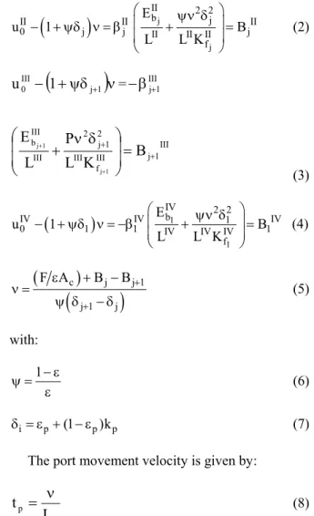
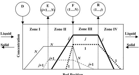
For a system of N components in which the components are numbered from low to high affinity as 1, ... , j, j+1, ..., N (Fig.2); and in which a split is desired between component j and j+1, the standing wave equations are as follows:
(
)
NN
I 2 2
b
I I N I
0 N N I I I N
f E
u 1 B
L L K
⎛ ψν δ ⎞
⎜ ⎟
− + ψδ ν = −β + =
⎜ ⎟
⎝ ⎠
(1)
(
)
jj
II 2 2
b j
II II II
0 j j II II II j
f E
u 1 B
L L K
⎛ ψν δ ⎞
⎜ ⎟
− + ψδ ν = β + =
⎜ ⎟
⎝ ⎠
(2)
(
+ψδ)
ν− j+1
III
0 1
u =−βIIIj+1
III 1 j III f III
2 1 j 2 III
III b
B K
L P
L E
1 j 1
j
+
+ =
⎟ ⎟ ⎠ ⎞ ⎜
⎜ ⎝
⎛ ν δ
+
+ +
(3)
(
)
11
IV 2 2
b
IV IV 1 IV
0 1 1 IV IV IV 1
f E
u 1 B
L L K
⎛ ψν δ ⎞
⎜ ⎟
− + ψδ ν = −β + =
⎜ ⎟
⎝ ⎠
(4)
(
)
(
c j 1 j j)
j 1F A B B+
+
ε + −
ν =
ψ δ − δ (5)
with:
1− ε
ψ =
ε (6)
i p (1 p)kp
δ = ε + − ε (7)
The port movement velocity is given by:
c p
L t = ν
(8)
II
IV I
III F
E R
D Liquid
C0III
CLIII
CLIV
C0I
CLI
C0II
CLII
CAR, CBR
CAE, CBE
CAF, CBF
C0IV
II
IV I
III F
E R
D Liquid
C0III
CLIII
CLIV
C0I
CLI
C0II
CLII
CAR, CBR
CAE, CBE
CAF, CBF
C0IV
D E R
Zone III Zone IV Zone II
Zone I
Liquid Liquid
Solid Solid
1 1
j+1
N
(j+1…N) (1…j)
j
N
j+1
(1…N) F
N
1
j+1
j j
Bed Position
Con
cen
tration
Figure 2: Standing wave theory, non-equilibrium model.
The β values are determined from a pseudo-binary model, where mixtures A and B are treated as single solutes A and B (Cremasco and Wang, 2000a). The four β values can be estimated from simple material balances around zones and mixing points. The following assumptions are made: (i) the concentration of solute A at the outlet of zone III is equal to its concentration at the raffinate port;(ii) the concentration of solute B at the inlet of zone II is equal to its concentration at the extract port; (iii) the ratio between the highest and the lowest concentrations for mixture (A or B) is the same in both adsorption and desorption zones. These assumptions lead to the following expressions:
R III F
IV A 0 A F II
1 II E j
0 A
C u C u
ln
u C
⎛ − ⎞
β = ⎜⎜ ⎟⎟= β
⎝ ⎠ (9)
E II F
I B 0 B F III
N III R j 1
0 B
C u C u
ln
u C +
⎛ + ⎞
β = ⎜⎜ ⎟⎟= β
⎝ ⎠ (10)
where, in the pseudo-binary model (Cremasco and Wang, 2000a):
∑
== =
j i
1 i
F i F
A C
C
(11)
∑
=+ = =
N i
1 j i
F i F
B C
C
(12)
∑
== =
j i
1 i
R i R
A C
C
(13)
∑
=+ = =
N i
1 j i
E i E
B C
C (14)
The A and B mixture recoveries at the outlet ports are defined as
F A F
R A R mix A
C u
C u Y =
(15)
F B F
E B E mix B
C u
C u Y =
(16)
where uR ≡ R/(εAc) and uE ≡ E/(εAc) are the
equivalent raffinate and extract interstitial velocities. Mass balances for mixtures A and B are substituted into Eqs. (9) and (10) to give:
(
)
1 IIIIV II E mix 0 mix
1 j II A A
R 0
u u
ln 1 Y Y 1
u u
−
⎧⎛ ⎞ ⎡⎛ ⎞ ⎤⎫
⎪ ⎪
β = β = ⎨⎜⎜ ⎟⎟ − ⎢⎜⎜ ⎟⎟ − ⎥⎬
⎢ ⎥
⎪⎝ ⎠ ⎣⎝ ⎠ ⎦⎪
⎩ ⎭
(17)
(
)
1 III III R mix 0 mix
N j 1 III B B
E 0
u u
ln 1 Y Y 1
u u − + ⎧⎛ ⎞ ⎡⎛ ⎞ ⎤⎫ ⎪ ⎪
β = β = ⎨⎜⎜ ⎟⎟ − ⎢⎜⎜ ⎟⎟ + ⎥⎬
⎢ ⎥
⎪⎝ ⎠ ⎣⎝ ⎠ ⎦⎪
⎩ ⎭
(18)
Substituting Eqs. (20) and (21) into (1) through (4), one obtains:
(
+ψδ)
ν− N
I
0 1
u =
(
)
⎪⎭ ⎪ ⎬ ⎫ ⎪⎩ ⎪ ⎨ ⎧ ⎥ ⎥ ⎦ ⎤ ⎢ ⎢ ⎣ ⎡ + ⎟⎟ ⎠ ⎞ ⎜⎜ ⎝ ⎛ − ⎟⎟ ⎠ ⎞ ⎜⎜ ⎝ ⎛ − 1 Y u u Y 1 u u
ln Bmix
E II 0 1 mix B III 0 R I N I f I 2 N 2 I I b B K L L E N N = ⎟ ⎟ ⎠ ⎞ ⎜ ⎜ ⎝
⎛ ψν δ
+ (19)
(
+ψδ)
ν− j
II
0 1
u =
(
)
⎪⎭ ⎪ ⎬ ⎫ ⎪⎩ ⎪ ⎨ ⎧ ⎥ ⎥ ⎦ ⎤ ⎢ ⎢ ⎣ ⎡ − ⎟⎟ ⎠ ⎞ ⎜⎜ ⎝ ⎛ − ⎟⎟ ⎠ ⎞ ⎜⎜ ⎝ ⎛ − 1 Y u u Y 1 u u
ln Amix
R III 0 1 mix A II 0 E II j II f II 2 j 2 II II b B K L L E j j = ⎟ ⎟ ⎠ ⎞ ⎜ ⎜ ⎝
⎛ ψν δ
+ (20)
(
+ψδ)
ν− j+1
III
0 1
u =
(
)
⎪⎭ ⎪ ⎬ ⎫ ⎪⎩ ⎪ ⎨ ⎧ ⎥ ⎥ ⎦ ⎤ ⎢ ⎢ ⎣ ⎡ + ⎟⎟ ⎠ ⎞ ⎜⎜ ⎝ ⎛ − ⎟⎟ ⎠ ⎞ ⎜⎜ ⎝ ⎛
− − Y 1
u u Y 1 u u
ln Bmix
E II 0 1 mix B III 0 R III 1 j III f III 2 1 j 2 III III b B K L L E 1 j 1 j + + = ⎟ ⎟ ⎠ ⎞ ⎜ ⎜ ⎝
⎛ ψν δ
+
+ +
(21)
(
+ψδ)
ν− 1
IV
0 1
u =
(
)
⎪⎭ ⎪ ⎬ ⎫ ⎪⎩ ⎪ ⎨ ⎧ ⎥ ⎥ ⎦ ⎤ ⎢ ⎢ ⎣ ⎡ − ⎟⎟ ⎠ ⎞ ⎜⎜ ⎝ ⎛ − ⎟⎟ ⎠ ⎞ ⎜⎜ ⎝ ⎛
− − Y 1
u u Y 1 u u ln mix A R III 0 1 mix A II 0 E IV 1 IV f IV 2 1 2 IV IV b B K L L E 1 1 = ⎟ ⎟ ⎠ ⎞ ⎜ ⎜ ⎝
⎛ ψν δ
+ (22)
The following expression is obtained from Eq. (5) and can be used to calculate the apparent adsorbent velocity
(
1 2)
2
1 λ ± λ
=
ν (23)
where:
(
)
II 1f II 2 j II j III 1 fj III 2 1 j III 1 j j 1 j 1 j K L K L − + + + + ⎟⎟ ⎠ ⎞ ⎜ ⎜ ⎝ ⎛ δ β + δ β δ − δ =
λ (24)
EXPERIMENTAL SECTION
Materials
HPLC grade acetonitrile was purchased from Fisher Scientific (Fairlawn, NJ). HPLC grade tetrahydrofuran (THF) was obtained from Sigma Chemical Co. (St. Louis, MO). Pure ethanol was purchased from McCormick Distilling Co. (Weston, MA). The ethanol was degassed prior to use by sonicating in an ultrasonic bath (Fairlawn, NJ). Distilled deionized water (DDW) was obtained from a Milli-QTM system by Millipore (Bedford, MA). All solvents used were filtered through 0.2-μm Nylon 66 filter from Alltech (Deerfield, IL). A taxane crude was generously provided by Bristol-Myers Squibb Co. (Syracuse, NY). The crude was derived from plant tissue culture broth through several proprietary purification and concentration steps. The polystyrene divinyl-benzene copolymer adsorbent (Dow XUS 43493) used in all low-pressure liquid chromatography (LPLC) and SMB columns was donated by Dow Chemical Co. (Midland, MI).
Instrumentation
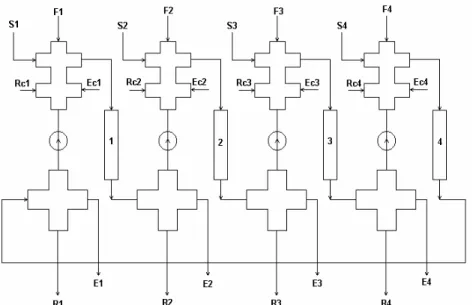
The laboratory-scale, four-column SMB used in all experiments is shown in Fig. 3. This unit had four pumps (two Pharmacia P-500 FPLC pumps and two Waters 510 HPLC pumps), a liquid chromatography controller (Pharmacia LCC-500), six rotary valves, four way valves (both of the four-way and six-way valves are from Alltech Associates, Inc., Deerfield, IL), and PTFE connection tubing. The LCC-500 controller was used to set each FPLC pump flow rate and each MV-8 valve position. Two
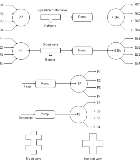
FPLC pumps were used to deliver feed and desorbent streams, and the two HPLC pumps were used to recycle part of the raffinate and extract streams. The MV-8 valves were used to direct the flow of each liquid stream and, therefore, control the inlet and outlet streams of each column (Fig.4). One of the MV-8 valves was used to control the feed stream and is called valve 1F. It had one inlet (from the FPLC feed pump) and four outlets (each of which led to one of the four columns). Similarly, valve 4S had one inlet (from the LPLC desorbent pump) and four entries (one of each column). Valve 2R was used to withdraw the raffinate. It had four inlets connecting each of the columns and one outlet connecting the raffinate withdrawing port. Valve 3Rc was used to recycle part of the raffinate stream back to zone II. Similarly, valve 5E was used to withdraw extract, and 6Ec was used to recycle part of the extract stream.
The valve positions connected with column 1, column 2, column 3, and column 4 were called position 1, 3, 5, and 7, respectively. There were also four one-way (on-off) valves to control the flow directions. The combination of these rotary valves and on-off valves effectively controlled all of the liquid flows. For example, if the feed was loaded into column 1 (F1 open) in Fig. 3, the position for valve 1F will be set to 1. Following the liquid flow, the raffinate was withdrawn (R2 open, 2R in position 3), and the on-off valve between R2 and Rc2 was closed to prevent Rc2 from going back to stream R2 (Rc2 open, 3Rc in position 3). The desorbent was added into column 3 (S3 open, valve 4S in position 5).The extract was then withdrawn (E4 open, 5E in position 7), and the on-off valve between E4 and Ec4 is closed to prevent Ec4 from going back to the E4 stream (Ec4 open, 6Ec in position 7).
Figure 4: Valve configuration in the laboratory-scale SMB.
Methods
Before SMB experiments, the crude mixture was dissolved in 60:40 ethanol:water v/v. When passed through a C18 HPLC column, the resulting chromatogram showed three major impurities: Tr21, Tr18, and Tr10 (the impurities were named on the basis of their retention times in the HPLC chromatogram). Paclitaxel had a retention time of 12 min in the HPLC chromatogram and it was also named Tr12. In the batch elution experiments, the impurities, which have HPLC retention times of 5 min, 9.5 min, and 16 min (denoted as Tr5, Tr9.5, and Tr16), were found to have very similar elution behavior in the Dow columns as Tr21, and these four components were treated as a single pseudo-component with the same properties as Tr21.
In SMB processes, HPLC was used to analyze the collected fractions and construct (off-line) the effluent concentration history. The HPLC system consisted of two pumps (Waters 510), a tunable single-wavelength detector (Waters 486) and an
injector (Waters U6K). Waters Millennium 2010 software was used for data collection. A Waters Nova-Pak C18 column and a premixed mobile phase of water:acetonitrile:tetrahydrofuran (60:30:10 v/v/v), at a flow rate of 1.0 ml/min were used. The
sample injection volume was 10μl. The
In SMB experiments, all of the feed and desorbent were degassed prior to all experiments. At the beginning of an experiment, the valves were set to the positions as configuration I. The FPLC pumps (for the introduction of feed and eluent) were started before the HPLC pumps (for recycling portions of the raffinate and extract products). At the end of an experiment, each column was flushed with enough eluent to remove all remaining solutes. At the end of the cleanup, a sample was collected from the outlet of each column. The samples were then analyzed with HPLC to make sure no residues remained.
RESULTS AND DISCUSSION
In order to obtain the flow rates and the switching time (or operating parameters) for LMS experiments, the linear standing wave analysis (LSWA) was used with the following steps:
1) Find column and particle characteristics (D, Lc, ε, dp, εp) – Table 1 in this work.
2) Find the partition coefficient kp (linear
isotherm) for each solute and identify the less-retained mixture A= 1, ..., j and the more-less-retained mixture B = j+1, ..., N. In this paper, this information is given in Table 2 (Cremasco et al., 2000b). From this table, for Run 1, it is specified that paclitaxel, Tr18, and Tr21 are the mixture A, and they are recovered at the raffinate outlet. In this same Run, the compound Tr10 is characterized as Mixture B, and it is recovered at the extraction outlet. Based on Table 2, for Run 2, it was specified that Tr21 is the mixture A, and it is recovered at the raffinate outlet, while the compounds paclitaxel and Tr18 are characterized as Mixture B, and they are recovered at the extraction outlet.
3) Find rate parameters (DAB, Dp, kfj, Ebj) – Table
2 for DAB, Dp in this work. The values of kfj and Ebj
depend on the flow rate in zone j. In this work, the axial dispersion coefficient Eb can be estimated from
a correlation by Athalye et al. (1992):
1 6 j p 0
j j
p 0 b
AB d u
E d u
(1 )D
⎡ ε ⎤
⎢ ⎥
=
− ε
⎢ ⎥
⎣ ⎦
(26)
and the parameters associated with the corrections for mass-transfer effects, given in Eqs. (1) to (4) can be calculated from (Ma et al., 1996b):
p P
2 p j
f p j
f 60 D
d
k 6
d
K 1
ε +
= (27)
where the film mass-transfer coefficient is calculated from a correlation by Wilson and Geankoplis (1966):
1 3
j j
p f p 0
AB AB
d k 1.09 d u
D D
⎛ ε ⎞
⎜ ⎟
= ⎜ ⎟
ε ⎝ ⎠
(28)
4) Fix the feed concentrations CAF and CBF. From
step 1 and Table 3; in this work for Run 1: CA F
= 332.7 ppm and CBF = 14.4 ppm.
5) Fix the mixture A yield at the raffinate port (YAmix) and the mixture B yield at the extract port
(YBmix). The values of YAmix and YBmix are fixed at
0.99 for Run 1.
6) Choose a feed flow rate F.
7) Calculate the liquid apparent interstitial velocity in each zone and simulated adsorbent velocity using Eqs. (1) to (4), assuming B1 = Bj =
Bj+1 = BN = 0.
8) Calculate the flow-rate values dependent on mass transfer parameters using the velocities calculated from step 6 and the correlations in step 3.
9) Calculate the new liquid apparent interstitial velocity in each zone j, and simulated adsorbent velocity.
10) Calculate the convergence criteria given by
(
)
(
)
≤⎥ ⎥ ⎦ ⎤ ⎢
⎢ ⎣ ⎡
ν − ν +
− −
=
=
∑
−2 1
2 1 k k 2 4
j
1 j
j 0 j 0k u k1
u 0.1×10⁻⁶ (29)
where k is the iteration number, and j is the zone number.
11) Calculate the restriction λ2≥ 0, Eq. (25). If this restriction is obeyed, then returns to step 6 and increases F. When λ2 < 0, the F value in the previous iteration is the maximum feed flow rate (Fmax).
12) Determine zone flow rates and port switching time.
Table 1: Column and particle characteristics
Parameter Value
Packed bed height, each column 12.3 cm
Column inner diameter 1.50 cm
Average bed void fraction 0.32
Particle void fraction 0.46
Average particle diameter 240 μm
Table 2: Partition and diffusivity coefficients (Cremasco et al., 2000b).
Component kp
(ml/ml solid volume)
DAB
(104 cm2/min)
Dp
(104 cm2/min)
Tr21 15.09 2.526 0.384
Tr18 38.67 2.564 0.920
Paclitaxel 40.03 2.560 0.590
Tr10 82.52 2.569 1.310
Table 3: Feed concentrations for run #1
Component Feed concentration (ppm)
Tr21 192.3 Tr18 19.6 Paclitaxel 120.8 Tr10 14.4
Table 4: Operating parameters for run #1
Parameter Value
YA 99.0
YB 99.0
Feed (ml/min) 0.178
Eluent (ml/min) 1.472
Raffinate (ml/min) 0.748
Extract (ml/min) 0.902
Zone I (ml/min) 1.808
Zone II (ml/min) 0.906
Zone III (ml/min) 1.070
Zone IV (ml/min) 0.322
Step time (min) 494.4
0 5 10 15 20 25 30 35 40 45 50
0 500 1000 1500 2000 2500 3000
Time (min)
Tr21 Tr18 Taxol a
0 5 10 15 20 25 30 35 40 45 50
0 500 1000 1500 2000 2500 3000
Time (min)
Tr21 Tr18 Taxol a
(a)
0 1 2 3 4
0 500 1000 1500 2000 2500 3000
Time (min)
Tr10 Tr21 Tr18 Taxol b
0 1 2 3 4
0 500 1000 1500 2000 2500 3000
Time (min)
Tr10 Tr21 Tr18 Taxol b
(b)
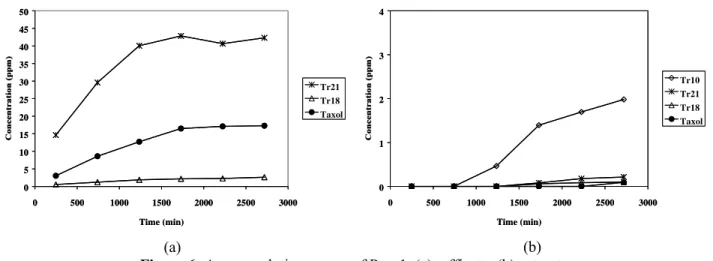
Figures 6a and 6b show elution curves based on the average product concentration, where each data point is taken at an interval of time equal to tp/2.
Figure 5a shows that mixture A (which includes paclitaxel) goes to the raffinate, which is free of Tr10. Tr10 migrates toward the extract port. The yield and purity of paclitaxel in the first pass were 86.2% and 27.8%, respectively. The low purity is due to the (expected) high concentration of Tr21 in the raffinate port. The SMB was designed to remove the high-affinity components in the extract and leave the low-affinity components (paclitaxel + impurities) in the raffinate.
The last four samples of the second half-step times of the raffinate product were taken as a new feed for Run 2 (Table 5) because the concentrations of these samples was sufficiently high to be used as feed to a second ring. The second feed mixture is composed of paclitaxel, Tr18 and Tr21. Paclitaxel and Tr18 were treated as a heavy pseudo-component (mixture B) and Tr21 as a light component (mixture A) in steps 2 and 4 in the algorithm presented for Run 1. Fixing YAmix and YBmix both equal to 0.9999
in step 5 of the same algorithm, the standing wave analysis was applied to calculate the operating parameters for Run 2 (Table 6). But paclitaxel and Tr18 are difficult to separate using the chosen adsorbent, because the selectivity between the two solutes is close to one (αpac,Tr18≡kp,pac/kp,Tr18 = 1.035).
With the same procedure as for Run 1 and the parameters from Table 6, the elution curves for Run 2 were obtained (Figs. 7a and 7b). In this run, there is a high paclitaxel concentration in the first half of the extract history (paclitaxel has the highest affinity in the extract stream). Figures 8a and 8b show the elution curves based on an average concentration, where each point represents an average over a time period equal to tp/2. Recovery and purity of
paclitaxel were 82.2% and 71.1%, respectively. Notice an improvement for purity, from 27.8% to 71.1%, when one compares the paclitaxel purity for Run 2 with that from Run 1. But 28.9% of the impurities are due to Tr21. Although the SMB operating conditions were assigned to force this component to migrate toward the raffinate port (Fig. 8a), some of it eluted at the extract port.
0 5 10 15 20 25 30 35 40 45 50
0 500 1000 1500 2000 2500 3000
Time (min)
Tr21 Tr18 Taxol a
0 5 10 15 20 25 30 35 40 45 50
0 500 1000 1500 2000 2500 3000
Time (min)
Tr21 Tr18 Taxol a
(a)
0 1 2 3 4
0 500 1000 1500 2000 2500 3000
Time (min)
Tr10 Tr21 Tr18 Taxol b
0 1 2 3 4
0 500 1000 1500 2000 2500 3000
Time (min)
Tr10 Tr21 Tr18 Taxol b
(b)
Figure 6: Average elution curves of Run 1: (a) raffinate; (b) extract.
Table 5: Feed composition for run #2.
Component Concentration (ppm)
Table 6: Operating parameters for run #2.
Parameter Value
YA 99.99
YB 99.99
Feed (ml/min) 0.33
Eluent (ml/min) 1.284
Raffinate (ml/min) 0.529
Extract (ml/min) 1.085
Zone I (ml/min) 1.711
Zone II (ml/min) 0.626
Zone III (ml/min) 0.994
Zone IV (ml/min) 0.415
Step time (min) 320.5
0 5 10 15 20 25 30
0 500 1000 1500 2000 2500
Time (min)
Tr21 Tr18 Taxol a
0 5 10 15 20 25 30
0 500 1000 1500 2000 2500
Time (min)
Tr21 Tr18 Taxol a
(a)
0 1 2 3 4 5 6 7 8
0 500 1000 1500 2000 2500
Time (min)
Tr21 Tr18 Taxol b
0 1 2 3 4 5 6 7 8
0 500 1000 1500 2000 2500
Time (min)
Tr21 Tr18 Taxol b
(b)
Figure 7: Elution curves of Run 2: (a) raffinate; (b) extract.
0 5 10 15 20 25 30
0 500 1000 1500 2000 2500
Time (min)
Tr21 Tr18 Taxol a
0 5 10 15 20 25 30
0 500 1000 1500 2000 2500
Time (min)
Tr21 Tr18 Taxol a
(a)
0 1 2 3 4 5 6 7 8
0 500 1000 1500 2000 2500
Time (min)
Tr21 Tr18 Taxol b
0 1 2 3 4 5 6 7 8
0 500 1000 1500 2000 2500
Time (min)
Tr21 Tr18 Taxol b
(b)
Figure 8: Average elution curves of Run 2: (a) raffinate; (b) extract.
CONCLUSION
This study demonstrates that a small batch (less than one liter) can be used to determine the feasibility of an SMB operation. In this paper, it was shown that a multicomponent and complex system,
experimental steps of separation.
One SMB experiment (with two passes) was performed to determine the purity and yield resulting from the specified operating conditions. Although the system employed had just four short columns (1.50 cm I.D. × 12.5 cm each) and the particles were large (150 to 300 μm in diameter), paclitaxel was recovered from the complex plant tissue culture broth in 82% yield and 72% purity.
NOMENCLATURE
Ac Column cross-sectional area L2
Ci Solute i concentration in the
inlet or outlet flow rate
ML–3
D Column diameter L
D Eluent (desorbent) flow rate L3T–1
DAB Free diffusion coefficient L2T–1
dp Average particle diameter L
Dp Effective pore-phase
diffusion coefficient
L2T–1
E Extract flow rate L3T–1
Eb Axial dispersion coefficient L2T–1
F Feed flow rate L3T–1
kf Film mass transfer
coefficient
LT–1 1/Kf Global mass transfer
resistance
T
kp Equilibrium partition
constant
L Zone length L
Lc Column length L
Q Zone flow rate L3T–1
R Raffinate flow rate L3T–1
tp Switching time T
tR Retention time T
u Liquid apparent interstitial velocity
LT–1 u0 SMB liquid interstitial
velocity
LT–1
v0 Pulse liquid superficial velocity LT
–1 Greek Letters
β Mass transfer correction in
the standing wave analysis
δ Adsorption velocity
ε Bed porosity;
εp Particle porosity;
ν Desorbent simulated
velocity;
ψ Bed porosity ratio
Subscripts
A Solute A (low-affinity)
B Solute B (high-affinity)
E Extract
F Feed
i Solute I
j Zone index
wave Solute concentration stationary wave
R Raffinate
Superscripts
E Extract
F Feed
j Zone index
R Raffinate
I Zone I
II Zone II
III Zone III
IV Zone IV
ACKNOWLEDGMENTS
This paper is part of Dr. Cremasco’s post-doctoral program, supported by the Sao Paulo State Foundation (FAPESP - n.98/03206-7) and by the State University of Campinas, Brazil. The authors gratefully acknowledge the support of Bristol-Myers Squibb Co. for providing the PTC broth.
REFERENCES
Athalye, A. M., Gibbs, S. J., and Lightfoot, E. N., Predictability of Chromatographic Protein Separations: Study of Size-exclusion Media with Narrow Particle Size Distribution, J. Chrom., 589, p. 71 (1992).
Berninger, J. A., Whitlhey, R. D., Zhang, X., and Wang, N.-H. L., A Versatile Model for Simulation of Reaction and Nonequilibrium Dynamics in Multicomponent Fixed-bed Adsorption Process, Computer Chem. Engng, 15 (11), p. 749 (1991).
Cardelina, J. H. II., HPLC Separation of Taxol and Cephalomannine, J. Liq. Chromatogr. Sci., 14 (4), p. 659 (1991).
Chemical Engineering Meetin, CD ROM, Santiago, Chile, 2000a.
Cremasco, M. A., Wu, D.-J. and Wang, N.-H. L., Estimation of Partition Coefficient and Mass-Transfer Parameters of Taxanes. (in Portuguese), XIII Brazilian Chemical Engineering Meeting, CD ROM, Águas de São Pedro, Brazil, 2000b.
Fett-Netto, A. G., DiCosmo, F., Reynolds, W. F., and Sakata, K., Cell Culture of Taxol Yield as a Source of the Antineoplastic Drug Taxol and Related Taxanes, Bio/Tecnology, 10, p. 1572 (1992).
Ma, Z., Au, B. W. and Wang, N.-H, L., Estimation of Solvente-Modulated Linear Adsorption Parameters of Taxanes from Dilute Plant Tissue Culture Broth, Biotechnolo Prog., 12, (6), p. 810 (1996).
Ma, Z., Whitley, R. D., and Wang, N.-H. L., Pore and Surface Diffusion in Multicomponent Adsorption and Liquid Chromatography Systems, AIChE J., 42, p. 1244. (1996b).
Mallmann, T., Burris, B. D., Ma, Z., and Wang, N. H. L., Standing Wave Design of Nonlinear SMB Systems for Fructose Separation. AIChE J., 44, (12), p. 2628 (1998).
Srinivasan, V., Pestchanker, L., Moser, S., Hirasuna,
T. J., Taticek, R., e Shuler, M. L., Taxol Production in Bioreactors: Kinetics of Biomass Accumulation, Nutrient Uptake, and Taxol Production by Cell Suspensions of Taxus baccata, Biotechnol. Bioeng., 47, p. 666 (1994).
Whitley, R. D., Dynamics of Nonlinear Multicomponent Chromatography-Interplay of Mass-Transfer, Intrinsic Sorption Kinetics, and Reaction. PhD thesis, Purdue University, West Lafayette, IN., USA (1990).
Wilson, E. J., and Geankoplis, C. J., Liquid Mass Transfer at Very Low Reynolds Numbers in Packed Beds, Ind. Eng. Chem. Fundam., 5, p. 9 (1966).
Wu, D.-J., Ma, Z., Au, B. W. and Wang, N.-H, L., Recovery and Purification of Paclitaxel Using Low-Pressure Liquid Chromatography, AIChE J., 3, (1), p. 232 (1997).
Wu, D-J., Xie, Y., Ma, Z. and Wang, N.-H. L., Design of Simulated Moving Bed Chromatography for Amino Acid Separations, Ind. Eng. Chem. Res., 37, p. 4023 (1998).